Allocative and Dynamic Efficiency in NBA Decision Making
←
→
Page content transcription
If your browser does not render page correctly, please read the page content below
MIT Sloan Sports Analytics Conference 2011
                                                                                               March 4-5, 2011, Boston, MA, USA

       Allocative and Dynamic Efficiency in NBA Decision Making

                                       Matt Goldman                                 Justin M. Rao
                                       UC San Diego                              Yahoo! Research Labs
                                     La Jolla, CA 92093                         Santa Clara, CA 95054
                                    mrgoldman@ucsd.edu                          jmrao@yahoo-inc.com

                                                                Abstract

       This paper examines the optimality of the shooting decisions of National Basketball Association (NBA)
       players using a rich data set of shot outcomes. The decision to shoot is a complex problem that involves
       weighing the continuation value of the possession and the outside option of a teammate shooting. We
       model this as a dynamic mixed-strategy equilibrium. At each second of the shot clock, dynamic efficiency
       requires that marginal shot value exceeds the continuation value of the possession. Allocative efficiency
       is the additional requirement that at that “moment", each player in the line-up has equal marginal
       efficiency. To apply our abstract model to the data we make assumptions about the distribution of
       potential shots. We first assume nothing about the opportunity distribution and establish a strict nec-
       essary condition for optimality. Adding distributional assumptions, we establish sufficient conditions
       for optimality. Our results show that the “cut threshold" declines monotonically with time remaining
       on the shot clock and is roughly in line with dynamic efficiency. Over-shooting is found to be rare,
       undershooting is frequently observed by elite players. We relate our work to the usage curve literature,
       showing that interior players face a generally steeper efficiency trade off when creating shots.

1     Introduction
Mixed strategy Nash equilibrium (MSNE) is a workhorse in modern game theory. Decision making in a dynamic
environment that involves weighing a current alternative versus the continuation value of a process of random
arrivals underlies both decision theoretic problems such as search and game theoretic problems such as bilateral
bargaining. In this paper we take these concepts to a difficult problem: shot choice in professional basketball. In
the National Basketball Association (NBA) a 5-man line-up has 24 seconds to take the best shot possible. To do
so the team must allocate the ball effectively across its factors of production (players) and over the course of the
shot clock. Decisions must be made quickly and sub-optimal choice can be the difference between winning and
losing. Equilibrium requires effective randomization across the 5-man line-up (allocative efficiency) and accurately
weighing the continuation value of a possession versus the value of a current opportunity (dynamic efficiency). We
employ rich data set comprising all shots taken in the NBA from 2006 to 2010 to fit our model of shot allocation
and optimal stopping to observed shooting behavior.
    Past work testing MSNE in field settings has studied 2x2 games such as soccer penalty kicks [1, 2, 3].1 Studying
a more complex game does come at a cost; it is also more challenging to fit into the confines of an abstract game-
theoretic model. Our approach is to combine the stopping problem with the allocation problem. At each point
on the shot clock, players must randomize across who shoots in order to maximize allocative efficiency and also
   1 The only work we are aware of that applies an optimal stopping model to professional sports is Romer (2006) [4], which examines NFL

coaches’ decisions to “go for it" on 4th down on the NFL. The difference is that this is a deliberative decision made perhaps 10 times per season
by the coach, not the players, and the low number of occurrences means coaches might intentionally do the wrong thing in order to adhere to
the “conventional wisdom".

                                                                       1
MIT Sloan Sports Analytics Conference 2011
March 4-5, 2011, Boston, MA, USA
use an appropriate threshold value for continuing the possession versus realizing a shot opportunity. The vector of
shooting frequency should maximize points per possession. This vector implies a “threshold equilibrium" of play,
in the spirit of a purified game [5].
The chief challenge in determining the optimality of player actions is to determine what would have happened
had the player shot less or more. Our model is flexible to the fact that certain players may be able to replicate their
average efficiency on marginal shots while other players may have to settle for much less efficient opportunities in
order to shoot more. Just as in the theory of the firm, it is the efficiency on these marginal opportunities that should
guide optimal allocation. Unfortunately, marginal opportunities are not readily observed. Understanding the
relationship between the marginal and average efficiencies of individual players has long been a contentious issue in
the basketball literature [6, 7, 8]. These relationships are often referred to as usage (or skill) curves and we have little
hope of interpreting the optimality of observed play without addressing them. Thus a key estimation challenge
we must confront, is to infer the “shot opportunity distribution" for each player. We start by assuming essentially
nothing about the shot opportunity distribution in order to achieve a necessary condition of optimality. We then
impose more restrictive, but still fairly flexible, assumptions in order to increase the power of our optimality tests
for allocative and dynamic efficiency. The goal is to apply the strictest test of optimality without incorporating a
misspecification into the abstract model.
Our key finding is that NBA players are superb optimizers. The average NBA player is shown to adopt reser-
vation shot values almost exactly equal to the continuation value of his team’s possession throughout the entire range
of the shot clock. Very few players can be shown to individually overshoot. Undershooting is far more common
and seems to occur primarily in players easily recognized as amongst the NBA elite. Such behavior is suboptimal in
our simple model, but is easily rationalized if we allow for such players to conserve their energy and health for the
long haul of the season at the slight expense of their team’s immediate performance. Most teams core line-ups show
impressive adherence to allocative efficiency, with a small spread in marginal efficiencies. We also find that NBA
experience is correlated with closer adherence to optimality for both dynamic and allocative efficiency. Salary is
positively correlated with departures from allocative efficiency, consistent with the idea that lower talent line-ups
have less margin for error.
Additionally our model yields estimates of the slope of each player’s usage curve. The estimates of any given
player contain lots of noise, but collectively they conform to the conventional intuitions about which kinds of
players are better at creating shots on the margin.
The paper proceeds as follows: Section 2 describes the data, Section 3 gives the model estimation and results
and Section 4 concludes.
2 Data
This analysis is entirely based on play-by-play data for NBA games from 2006-2010 (four seasons). The game logs
detail all the players on the court the outcome of every play. All variables discussed herein are constructed (via
some fairly extensive coding) from the raw game logs.2 Approximately 100 games (out of the 4,920 played during
this time period) are missing from this data set. We have no reason to believe their omission is anything other than
random. Appendix Table 1 describes the data in more detail.
3 Model and Results
In this section, we first motivate our general model of basketball and then describe the general model of optimal
play. We assume risk-neutrality so that the offensive team’s objective is solely to maximize points per possession.
This assumption is justified due the large number of possessions per game and the central limit theorem. We
also eliminate clear cases where risk-neutrality is violated, such as end of quarter and end of game situations.
Additionally, this model applies only to half-court sets and not to fast breaks or actions taken immediately after
2 Basketballgeek.com has a database of game logs, taken from NBA.com reporting.
2MIT Sloan Sports Analytics Conference 2011
March 4-5, 2011, Boston, MA, USA
offensive rebounds (which involve fairly trivial allocation/timing decisions). We define a fast break as any possession
used within the first seven seconds of the offense and have purged all such possessions from the data. In the
Appendix, we present brief justifications for both of these assumptions. “Garbage time" has been purged from our
data as our model only applies to situations where the outcome of the game can reasonably be effected by chosen
offensive strategy. Finally, we are unable to correctly infer the value of the shot clock for possessions occurring
immediately after made field goals. The value of the shot clock is very important to our analysis, so we must throw
these possessions out. After these omissions, we are left with roughly 40% of all possessions.
3.1 General model
There are 674 distinct players in our four year sample, denote each one by i ∈ {1, ..., 674}. O ≡ {i: player i is on
offense}, D ≡ {i: player i is on defense}. Defensive strategy is summarized by the selection of five choice variables
{dj }j∈O which represent the average level of attention devoted to each offensive player across the possession. These
variables are constrained by the abilities of the defenders according to:
gD (dO1 , dO2 , dO3 , dO4 , dO5 ) ≤ 0 (1)
where g is an arbitrary function with strictly positive derivatives in all arguments.
At every one second long interval of the shot clock, each player has the opportunity to use a possession. With t
seconds remaining on the shot clock (t ∈ {0, 1, ..., 17}), player i draws an unbiased measure of the expected number
of points his team would get from his immediate use of the possession, ηi,t ∼ Φi,O/i,di ,t . This value represents not
just expected points on his immediate shot, but also whatever value his team is likely to get (including points scored
after offensive rebounds or from foul shots) before ending their possessions. ηi,t is also effected by the likelihood
that player i should turn the ball over in his attempt to use the possession. ∀i ∈ O, player i has the opportunity to
use the possession, getting on average a value of ηi,t for his team if he does so. If no player choses to exercise the
possession at interval t, than the one second long period of the shot clock is allowed to pass and each player will
realize new and independent scoring opportunities in period t-1. Note that we are not assuming a viable scoring
opportunity for every player at every interval of the shot clock, it is entirely possible that during many seconds of
the shot clock a player will realize scoring opportunities of arbitrarily small expected value. In period 0, the shot
clock is about to expire. If no player uses the possession during this period, then play is stopped and the ball is
awarded to the other team with no points for the offense. In principal, the distribution of scoring opportunities
could vary over player, teammates, interval of the shot clock, and the level of defensive attention. Understanding
the interrelationships between all of these variables is an important direction for our future work, but for now we
assume player i’s opportunity distribution is invariant to teammates (O/i) and defense (di,t ).
Definition of Variables
For some possibly singleton set I ∈ O and a possibly singleton and convex T ∈ {0, ..., 24}, define NI,T as the
number of shots used by players in I over elements of the shot clock in T and define PI,T as the total number of
points realized from these possessions. Further, let:
PI,T 0 0 NI,T
EI,T = ; T∗ = {t ∈ {0, ..., 24} : ∀t ∈ T, t < t }; UI,T = (2)
NI,T NO,T ∪T∗
E is a measure of average efficiency in the periods in T and U is the hazard rate with which possessions are used
over a particular interval T and by a particular subset of offensive players. Note that all of these variables describe
observed data, if we wish to describe the “true" efficiency or usage rate of a particular set of players over some
interval, we will use a lower case version of the same definitions (e, u).
3MIT Sloan Sports Analytics Conference 2011
March 4-5, 2011, Boston, MA, USA
General Solution
Each player i chooses a cut-off level, ci,t , such that he will use the possession at interval t if and only if ηi,t ≥ ci,t . If
∀i, ηi,t < ci,t than no player choses to use the possession and the team proceeds to the next period of the shot clock.
In order for a player’s choice of cutoff to be optimal it must meet two basic criteria. Allocative efficiency: At any
given t, the team cannot reallocate the ball to increase productivity on the margin. The frequency at which each
player shoots generates equal marginal productivity. Allocative efficiency generates the best set of shot opportunities,
because randomizing effectively is a best response to selective defensive pressure. Formally, allocative efficiency requires
that ∀i, j ∈ O, ci,t = cj,t . Dynamic efficiency: Conditional on allocating efficiently in future periods, a shot is
realized only if its expected value exceeds the continuation value of a possession. Formally, dynamic efficiency
requires that ∀i ∈ O, ci,t = eO,t∗ .
3.2 A Necessary Condition for Dynamic Optimality
In this section we develop a minimalistic necessary condition for dynamic optimality that makes no assumptions
about our opportunity distributions. We address the question, “Do players take shots too frequently and/or too
soon in the shot clock?" player i only shoots at t if ηi,t > ci,t . Thus: ei,t = E(ηi,t |ηi,t ≥ ci,t ) > ci,t . As such,
we take as a null hypothesis of dynamic efficiency that: eI,T ≥ eO,T∗ . In the appendix we derive the test statistic
for this hypothesis. Failing this test means a player’s average output is consistently below the continuation value
of the possession. We ran this test for all players in our sample with T = {12, ...17} (the largest amount of data)
and were only able to find a single player ( Joel Przybilla) who violated it at α = 0.05. These results indicate that
NBA players are not taking patently wrong actions. However, we note that the power of this test is quite weak.
Typically there is a divergence between a player’s “worst shot" and average shot, with the average shot necessarily
offering higher efficiency. Put another way, there may be much slack between their average efficiency (ei,t ) and
their marginal efficiency (ci,t ). If a player’s average is consistently below the continuation value, the team would be
better off if he did not shoot at all for the interval of the shot clock (his mistakes outweigh the benefit he provides).
Our results show that this optimality condition is rarely violated in NBA play.
3.3 Dynamic Efficiency Using Parametric Uniform Shot Distributions
The conditions of the previous section are quite permissive of potentially suboptimal play for two reasons: 1) they
provide no tests for undershooting 2) they give no insight toward allocative efficiency. Furthermore, they offer no
convenient way to characterize the overall distribution from which a player realizes scoring opportunities. In this
section we address these difficulties. In order to do so we must make a somewhat restrictive assumption. Namely
that ∀t ∈ {0, ..., 17} player i draws his opportunities from a common distribution. This will allow us to compare
player i’s performance at the beginning of the shot clock (when he will rarely shoot) to the end of the shot clock
(when he will have to shoot a much higher fraction of the time). Intuitively, we are using the shot clock as an
instrument to identify player i’s opportunity distribution and implied usage curve. Note that we have not included
the final two periods of the shot clock. It is our belief that the inability to make a pass before shooting in these
periods results in a fundamentally different game and different opportunity distributions. We model player i’s
scoring opportunities as drawn from a uniform distribution along the interval [Bi , Ai ]. Additionally, the player
selects a shot in period t if his draw lies in the interval of [ci,t , Ai ]. For the vast majority of players, Bi will take a
negative value. This does not mean that players have opportunities to lose points, but merely reflects the fact that
the vast majority of players do not realize a good scoring opportunity in most periods of the shot clock. As long as
ci,t > 0 the part of our theoretical uniform opportunity distribution that lies below zero is irrelevant. Conditional
4MIT Sloan Sports Analytics Conference 2011
March 4-5, 2011, Boston, MA, USA
on the parameters θi = {Ai , Bi , {ci,t }t∈T }, it is straightforward that:
Ai + ci,t Ai − ci,t dei,t
ei,t = , ui,t = , = Ai − Bi
2 Ai − Bi dui,t
Ai −ci,t Ai +ci,t
Y Ui,t − Ai −Bi Ei,t − 2
P rob({Ei,t , Ui,t }t∈T |θi , Ni,t ) = φ( q )φ( )
Ai −ci,t Ai −ci,t √σi
t∈T Ni,t Ai −Bi (1 − Ai −Bi ) Ni,t
The likelihood equation, is dependent upon the application of a central limit theorem to each individual period of
the shot clock. Thus we proceed by performing Maximum Likelihood Estimation (MLE) for every single player
with at least 15 used possessions in every relevant period of the shot clock.3 Figure 1 provides the aggregate
results of this estimation procedure. We see that indeed NBA players use a monotonically declining cut threshold
consistent with the predictions of an optimal stopping problem with finite periods. More impressive is the fact
that the cut-thresholds are nearly identical to the continuation values of the possession and the functions have the
same shape. We present the results in two panels to enhance the contrast of the slope, while still showing it for all
periods of the shot clock. Overall, Figure 1 is strong evidence in favor of near optimal play. NBA players appear to
be well-tuned to the continuation value of the possession and adjust their shot choice to reflect it. This is precisely
the mechanics of optimal stopping. Not only do they get the mechanics right, but the rate at which the players
lower their cut threshold matches the continuation value nearly exactly!
Figure 1: Estimated shooting thresholds (cut-points) and possession continuation values. Left panel: all periods of
the shot clock. Right panel: restricted to periods of the shot clock with 4 or more seconds remaining to visually
display the slope more clearly.
We do note, however, that in Figure 1 the cut-threshold does lie slightly above the continuation value, which is
evidence that undershooting is more common that overshooting. To extend the analysis, we now examine which
player’s tend to overshoot or undershoot on average. We take as a null hypothesis that each player is dynamically
3 Despite the fact that we are fitting a uniform distribution, the support of observed efficiency and usage rates over any finite sample does not
change so we do not have a regularity problem and are able to calculate standard asymptotic variances from the likelihood matrix. Additionally,
we achieve parametric identification because the likelihood matrix is non-singular for all players who choose at least some variation in cutoff
levels across periods of the shot clock. This should not be a surprise, if a player did the same thing in every period of the shot clock, we have no
hope of learning about his usage curve. Finally, we do not observe the true model lies within our specification and apply consistently estimated
covariance matrices to our results from White (1982).
5MIT Sloan Sports Analytics Conference 2011
March 4-5, 2011, Boston, MA, USA
P P
efficient on average. Namely that for each player i, t∈{0,..,17} ωt ci,t = t∈{0,..,17} ωt eO,t∗ . To maximize power
to detect deviation, we test this hypothesis with a weights inverse to the variance of our estimated cutoffs. Figure
2 provides a histogram of the resulting t-statistics. A negative t-statistic indicates overshooting, a positive t-statistic
indicates undershooting.
Figure 2: Player-by-player t-statistic for deviations from dynamic optimality. Positive values indicate “under-
shooting."
The results again indicate that undershooting is much more common than overshooting. In fact, only 5 players
are found to be significant over-shooters — less than we would expect to find by chance alone (although if we
take the mean to be 1, not 0, the evidence these players overshoot strengthens considerably.4 In line with this
reasoning, the distribution appears standard normal but shifted over about 1 (the mean 0.98) Most players appear
to be optimizing and mistakes tend to come in the form of undershooting early in the shot clock. In this sense,
some players wait too long to shoot or do not expend maximum effort on each possession. In contrast, lab subjects
tend to pull the trigger too early, typically through the use of a fixed threshold [9]. We also compute the loss
in surplus due to sub-optimal shooting decisions (intuitively integrating between the two lines in Figure 1). The
median value of DWL across players is 4%, consistent with nearly optimal play.
To investigate which factors lead to under/over-shooting we regress the t-stat from adherence to dynamic op-
timality on individual player characteristics and find that salary is positively related to the t-stat (coef 0.08 per M,
t = 2.75, p < .007). Indeed the league’s star players such as Chris Paul, Lebron James and Kobe Bryant have high
t’s. The fact that higher paid players are more likely to under shoot is perhaps surprising at first. For instance,
some readers might have the intuition that NBA players interests diverge from team interests in that they have
the incentive to raise their point average through suboptimal play. Under this view, the labor market rewards the
wrong attributes (points per game as opposed to efficiency, for example). Our results are inconsistent with the view
of labor market. Boosting individual production at a cost to the team does not seem to be a strategy frequently
employed by NBA players. We think this is interesting in its own right. Teams still have a principle-agent problem
in that long-term contracts create a moral hazard for effort, but it is interesting that very few players exhibit “selfish
play." Our belief is that the prevalence of under-shooting among the higher paid players is evidence that the better
players conserve energy at times due to their high playing time and long season (over-shooting would be impossible
to rationalize this way and we observe far less over-shooting).
3.4 Allocative Efficiency
Allocative Efficiency is the hypothesis that the players on the court, (I) use the same cut-point in all periods of the
shot clock. This implies they have equal marginal efficiencies; put another way, it means the team cannot reallocate
the ball to relatively more productive players on the margin and boost output per possession. In our estimation we
allow the the set I to be an entire five man lineup or a three or four man "core" that more frequently shares the
4 Lamar Odom, Monta Ellis, Rafer Alston, Russell Westbrook and Tyrus Thomas are the guilty parties.
6MIT Sloan Sports Analytics Conference 2011
March 4-5, 2011, Boston, MA, USA
court. The concept of cores is convenient to improve power in estimation Because our estimation is more precise
for these periods, we will focus on cut-points in the first thirteen seconds of the shot clock (T = {5...18}). Let c
be the kT kkIk × 1 vector of relevant cut points, sorted first by period of the shot clock. Based on our parametric
procedure we have: ĉ ∼ N (c, VNc ). We define the "true" deviation from Allocative Efficiency as spread.
− c¯t )2 = (c − c̄)0 I(c − c̄) = z 0 Iz
P P
SI,T = t∈T i∈I (ci,t
It turns out that the natural empirical analog to this measure is biased upwards in small samples, we show in
the Appendix that we can derive an unbiased estimator by making a relatively straightforward bias correction. We
use the de-biased measure of spread through the paper. In this section our analysis focuses on 3-man cores. Using
complete 5 man line-ups is untenable from a sample size perspective, the results from 3-man and 4-man cores do
not meaningfully differ, however the data is about 5 times larger for 3-man cores. We include in our analysis any
core of 3 players for which each player in the line-up takes at least 15 shots for every interval of the shot clock.
Table 1: Line-up characteristics and spread
Offensive Efficiency -0.0204
(0.0541)
Possessions 1.08e-05***
(2.57e-06)
Mean Salary 0.00559***
(0.00207)
S.D. Salary 1.38e-09
(2.22e-09)
Mean NBA Experience -0.00840***
(0.00213)
S.D. NBA Experience 0.000130
(0.00323)
Figure 3: Distribution of spread for 4-man Observations 1,307
cores. Higher values indicate larger *** pMIT Sloan Sports Analytics Conference 2011
March 4-5, 2011, Boston, MA, USA
3.5 Variation in the Usage Curve by Position
As noted above our parametric model also predicted the slope of the usage curve for each player as the length of
their uniform opportunity distribution ( Ai −B
2
i
). These predictions were noisy for individual players, but via a
secondary regression we can observe patterns in how the usage curve’s of individual players are related to their
primary position and their role within their offense (usage% is defined as the fraction of a team’s possessions a
given player uses). We use the standard convention for position numbering (1: point guard, 2: shooting guard, 3:
small forward, 4: power forward, 5: center.
Table 2: Robust OLS Regression Explaining the Usage Curve
LHS/RHS Point Guard Shooting Guard Small Forward Power Forward Center Usage %
Ai − ˆ Bi 5.02∗∗∗ 5.73∗∗∗ 5.61 ∗∗∗ 6.32∗∗∗ 6.52 ∗∗∗ -8.5∗∗∗
s.e. (0.52) (0.59) (0.58) (0.62) (0.65) (1.94)
R2 = 0.8465, *** pMIT Sloan Sports Analytics Conference 2011
March 4-5, 2011, Boston, MA, USA
5 Acknowledgments
This a shortened version of a longer paper called “He Got Game Theory? Optimal Decision Making and the
NBA" available at www.justinmrao.com. We would like to thank James Andreoni, Nageeb Ali, Vincent Crawford,
Gordon Dahl, David Eil, Uri Gneezy, Ivana Komunjer, Craig McKenzie, Joel Sobel, Charles Sprenger, William
Peterman, Pedro Rey Biel and David Woolston for helpful comments.
References
[1] P.-A. Chiappori, S. Levitt, and T. Groseclose, “Testing mixed-strategy equilibria when players are heteroge-
neous: The case of penalty kicks in soccer,” The American Economic Review, vol. 92, no. 4, pp. 1138–1151,
2002.
[2] I. Palacios-Huerta, “Professionals Play Minimax,” Review of Economic Studies, pp. 395–415, 2003.
[3] M. Walker and J. Wooders, “Minimax play at wimbledon,” The American Economic Review, vol. 91, no. 5,
pp. 1521–1538, 2001.
[4] D. Romer, “Do firms maximize? Evidence from professional football,” Journal of Political Economy, vol. 114,
no. 2, 2006.
[5] J. Harsanyi, “Games with randomly disturbed payoffs: A new rationale for mixed-strategy equilibrium points,”
International Journal of Game Theory, vol. 2, no. 1, pp. 1–23, 1973.
[6] B. Skinner, “The Price of Anarchy in Basketball,” Journal of Quantitative Analysis in Sports, vol. 6, no. 1, p. 3,
2010.
[7] D. Oliver, Basketball on paper: rules and tools for performance analysis. Brassey’s, 2004.
[8] D. Berri, “Who is most valuable? Measuring the player’s production of wins in the National Basketball Associ-
ation,” Managerial and Decision Economics, vol. 20, no. 8, pp. 411–427, 1999.
[9] M. Lee, T. O’connor, and M. Welsh, “Decision-Making on the Full Information Secretary Problem,” in Pro-
ceedings of the 26th annual conference of the cognitive science society, pp. 819–824, Citeseer, 2004.
9MIT Sloan Sports Analytics Conference 2011
March 4-5, 2011, Boston, MA, USA
6 Appendix
6.1 Tables
Appendix Table 1: Data Overview and Description
Event/Action Description
Offensive/defensive line-up Players on court at given time
Game-time Minutes and second of each event
Game day Date of game
Shooter Player/time of the action
Rebound/assist Player/time of the action
Foul Shooting, non-shooting, flagrant, illegal defense
x,y coordinate of shot Physical location of shot
Turnover Broken down by bad pass, dribbling error, charge, lost ball
6.2 Parametric Model Specification Tests
Our model is identified by assuming invariance of a player’s ability to realize scoring opportunities across different
values of the shot clock. However, because we make this assumption for 16 different periods of the shot clock, our
model is overidentified and our assumptions can be tested. Suppose for example that defenses became progressively
more tenacious over the course of the shot clock and that player’s opportunity distributions generally declined
across the shot clock. Then, we would find that a single distribution could not accurately reflect a players ability
to score in both the beginning and end of the shot clock. Players would end up shooting less and less efficiently
towards the end of the shot clock than our model would predict. For now, we present plots showing how our
model preforms across the shot clock as an average across all players in our sample. We take solace in the lack of
any obvious trends in our residuals.
6.3 Necessary condition derivation
A convenient test is implied by application of a central limit theorem, to give:
σI
EI,T ∼ N (eI,T , )
NI,T
σO
EO,T∗ ∼ N (eO,T∗ , )
NO,T∗
T ∩ T∗ = ∅ → EO,T∗ ⊥ EI,T
σO 2 σI 2
r
EI,T − EO,T∗ ∼ N (eI,T − eO,T∗ , ( ) +( )
NO,T∗ NI,T
10MIT Sloan Sports Analytics Conference 2011
March 4-5, 2011, Boston, MA, USA
6.4 Unbiased measure of spread
We defineP the "true" deviation from Allocative Efficiency as spread.
SI,T = t∈T i∈I (ci,t − c¯t )2 = (c − c̄)0 I(c − c̄) = z 0 Iz
P
Where ci,t is the cutoff chosen by player i in period t and c¯t is the average over the five teammates of the cutoff
chosen in period t and c̄ is the appropriate corresponding kT kkIk × 1 vector of averages.
Note that, if we define M = IT ⊗ (I5 − J55 ), we may also simply write z = M c and S = c0 M 0 M c = c0 M c.
The "seemingly" natural empirical analog to S is:
P5
Ŝ = t∈T i=1 (cˆi,t − cˆ ¯t )2 = ẑ 0 I ẑ
P
However, a little bit of calculation reveals that this measure is biased upwards, especially for small samples.
E(ẑ) = c − c̄
V (ẑ) ≡ Vz = M VNc M P
2
) = E(zˆi,t )2 + V (zˆi,t ) = S + diagVz = S + diag(M Vc M )
P P P
Thus: E(Ŝ) = E(zi,t N
turns out to be upward biased and especially so for small n. In order to correct for this, we essentially subtract off
the bias andPdefine:
Vˆc M )
Sˆ∗ = Ŝ − diag(M N
6.5 4-man Cores
6.6 Additional support for Risk Neutrality
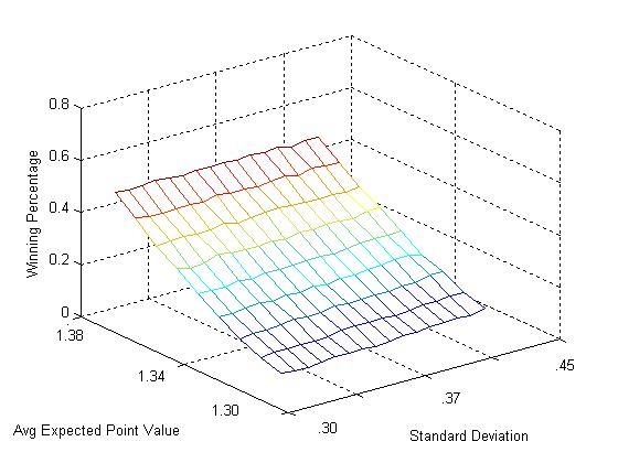
The following plot shows the simulated winning percentage for an underdog with baseline mean expected point
value of 1.38 playing a team who averages 1.4 points per possession with standard deviation 0.45. Each “game" was
simulated 10,000 times. As evidenced by the figure, although the underdog wants to increase the standard deviation
of the expected value of shot attempts it does not want to trade off any meaningful amount of mean to do so.
11MIT Sloan Sports Analytics Conference 2011
March 4-5, 2011, Boston, MA, USA
Appendix Figure 1: Underdog winning percentage as a function of standard deviation and mean
6.7 When Does Half-Court Offense Begin?
We decided that half-court offense began with 17 seconds on the shot clock. Our reason for doing so, is that prior
to 17 seconds the average value of exercising a possession is found to be strongly correlated with the mechanism by
which the possession originated (steal, dead ball, or defensive rebound). However, from 17 seconds on team’s are
in a half court set and the average value of possession use is now independent of how the possession originated.
12You can also read