Mastering Terra Mystica: Applying Self-Play to Multi-agent Cooperative Board Games
←
→
Page content transcription
If your browser does not render page correctly, please read the page content below
Mastering Terra Mystica: Applying Self-Play to Multi-agent Cooperative Board
                                                                           Games

                                                                                                            Luis Perez
                                                                                                        Stanford University
                                                                                                          450 Serra Mall
arXiv:2102.10540v1 [cs.MA] 21 Feb 2021

                                                                                                  luisperez@cs.stanford.edu

                                                                       Abstract                                        ent Factions 2 , different set of end-round bonus tiles being
                                                                                                                       selected.
                                             In this paper, we explore and compare multiple algo-                         TM is a game played between 2-5 players. For our re-
                                         rithms for solving the complex strategy game of Terra Mys-                    search, we focus mostly on the adversarial 2-player version
                                         tica, thereafter abbreviated as TM. Previous work in the                      of the game. We do this mostly for computational effi-
                                         area of super-human game-play using AI has proven ef-                         ciency, though for each algorithm we present, we discuss
                                         fective, with recent break-through for generic algorithms in                  briefly strategies for generalizing them to multiple play-
                                         games such as Go, Chess, and Shogi [4]. We directly apply                     ers. We also do this so we can stage the game as a zero-
                                         these breakthroughs to a novel state-representation of TM                     sum two-player game, where players are rewarded for win-
                                         with the goal of creating an AI that will rival human players.                ning/loosing.
                                         Specifically, we present initial results of applying AlphaZero                   TM is a fully-deterministic game whose complexity
                                         to this state-representation, and analyze the strategies de-                  arises from the large branching factor and a large number of
                                         veloped. A brief analysis is presented. We call this modified                 possible actions At from a given state, St . There is further
                                         algorithm with our novel state-representation AlphaTM. In                     complexity caused by the way in which actions can interact,
                                         the end, we discuss the success and short-comings of this                     discussed further in Section 1.2.
                                         method by comparing against multiple baselines and typi-
                                         cal human scores. All code used for this paper is available                   1.2. Input/Output Of System
                                         at on GitHub.                                                                     In order to understand the inputs and outputs of our sys-
                                                                                                                       tem, the game of TM must be fully understood. We lay out
                                                                                                                       the important aspects of a given state below, according to
                                         1. Background and Overview                                                    the standard rules [2].
                                                                                                                           The game of TM consists of a terrain board that’s split
                                         1.1. Task Definition                                                          into 9 × 13 terrain tiles. The board is fixed, but each terrain
                                                                                                                       tile can be terra-formed (changed) into any of the 7 distinct
                                            In this paper, we provide an overview of the infrastruc-                   terrains (plus water, which cannot be modified). Players can
                                         ture, framework, and models required to achieve super-                        only expand onto terrain which belongs to them. Further-
                                         human level game-play in the game of Terra Mystica (TM)                       more, TM also has a mini-game which consists of a Cult-
                                         [1], without any of its expansions 1 . The game of TM                         Board where individual players can choose to move up in
                                         involves very-little luck, and is entirely based on strategy                  each of the cult-tracks throughout game-play.
                                         (similar to Chess, Go, and other games which have re-                             The initial state of the game consists of players selecting
                                         cently broken to novel Reinforcement Learning such Deep                       initial starting positions for their original dwellings.
                                         Q-Learning and Monte-Carlo Tree Search as a form of Pol-                          At each time-step, the player has a certain amount of re-
                                         icy Improvement [3] [5]). In fact, the only randomness                        sources, consisting of Workers, Priests, Power, and Coin.
                                         arises from pregame set-up, such as players selecting differ-                 The player also has an associated number of VPs.
                                                                                                                           Throughout the game, the goal of each player is to ac-
                                            1 There are multiple expansions, most which consists of adding different   cumulate as many VPs as possible. The player with the
                                         Factions to the game or extending the TM Game Map. We hope to have
                                         the time to explore handling these expansions, but do not make this part of     2 A Faction essentially restricts each Player to particular areas of the

                                         our goal                                                                      map, as well as to special actions and cost functions for building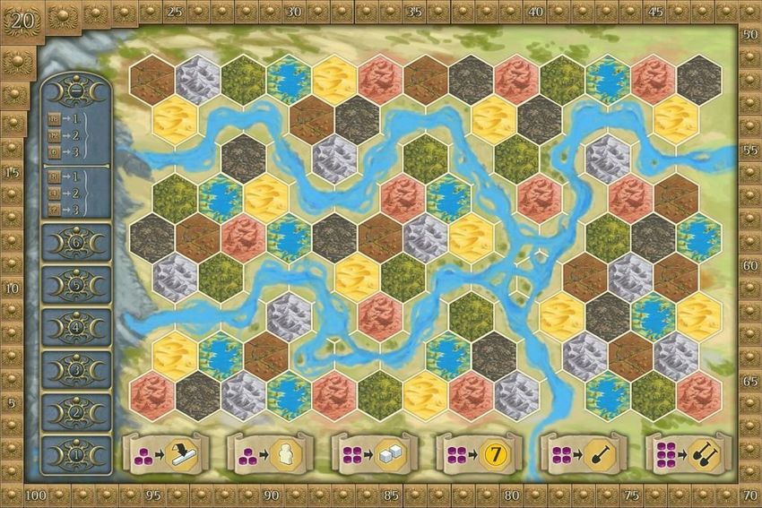
highest number of VPs at the end of the game is the winner.       1.3. Output and Evaluation Metrics
   From the definition above, the main emphasis of our sys-
                                                                     For a given state, the output of our algorithm will consist
tem is the task of taking a single state representation St at a
                                                                  of an action which the player can take to continue to the
particular time-step, and outputting an action to take to con-
                                                                  next state of the game. Actions in TM are quite varied, and
tinue game-play for the current player. As such, the input
                                                                  we do not fully enumerate them here. In general, however,
of our system consists of the following information, fully
                                                                  there are eight possible actions:
representative of the state of the game:
                                                                   1. Convert and build.
 1. Current terrain configuration. The terrain configura-
    tion consists of multiple pieces of information. For           2. Advance on the shipping ability.
    each terrain tile, we will receive as input:                   3. Advance on the spade ability.
      (a) The current color of the tile. This gives us in-         4. Upgrade a building.
          formation not only about which player currently
          controls the terrain, but also which terrains can        5. Sacrifice a priest and move up on the cult track.
          be expanded into.                                        6. Claim a special action from the board.
      (b) The current level of development for the ter-
                                                                   7. Some other special ability (varies by class)
          rain. For the state of development, we note that
          each terrain tile can be one of (1) UNDEVEL-             8. Pass and end the current turn.
          OPED, (2) DWELLING, (3) TRADING POST,                       We will evaluate our agents using the standard simula-
          (4) SANCTUARY, or (5) STRONGHOLD.                       tor. The main metric for evaluation will be the maximum
      (c) The current end-of-round bonus as well as future        score achieved by our agent in self-play when winning, as
          end-of-round bonus tiles.                               well as the maximum score achieved against a set of human
      (d) Which special actions are currently available for       competitors.
          use.
                                                                  2. Experimental Approach
 2. For each player, we also receive the following infor-
    mation.                                                          Developing an AI agent that can play well will be ex-
                                                                  tremely challenging. Even current heuristic-based agents
      (a) Current level of shipping ability, Current level of     have difficulty scoring positions. The state-action space for
          spade ability, the current number of VPs that the       TM is extremely large. Games typically have trees that are
          player has.                                             > 50 moves deep (per player) and which have a branching
      (b) The current number of towns the player has (as          factor of > 10.
          well as which town is owned), The current num-             We can approach this game as a typical min-max search-
          ber of worker available to the player, the current      problem. Simple approaches would simply be depth-limited
          number of coins available to the player, the cur-       alpha-beta pruning similar to what we used in PacMan.
          rent number of LV1, LV2, and LV3 power tokens.          These approaches can be tweaked for efficiency, and are es-
                                                                  sentially what the current AIs use.
      (c) The current number of priests available to the             Further improvement can be made to these approaches
          player.                                                 by attempting to improve on the Eval functions.
      (d) Which bonus tiles are currently owned by the               However, the main contribution of this paper will be to
          player.                                                 apply more novel approaches to a custom state-space rep-
      (e) The amount of income the player currently pro-          resentation of the game. In fact, we will be attempting to
          duces. This is simply the power, coins, priests,        apply Q-Learning – specifically DQNs (as per [3], [5], and
          and worker income for the player.                       [4]).
                                                                  2.1. Deep Q-Learning Methods for Terra Mystica
    The above is a brief summary of the input to our algo-
rithm. However, in general, the input to the algorithm is a           Existing open-source AIs for TM are based on combi-
complete definition of the game state at a particular turn.       nation of sophisticated search techniques (such as depth-
Note that Terra Mystica does not have any dependencies in         limited, alpha-beta search, domain-specific adaptations, and
previous moves, and is completely Markovian. As such,             handcrafted evaluation functions refined by expert human
modeling the game as an MDP is fully realizable, and is           players). Most of these AIs fail to play at a competitive
simply a question of incorporating all the features of the        level against human players. The space of open-source AIs
state.                                                            is relatively small, mainly due to the newness of TM.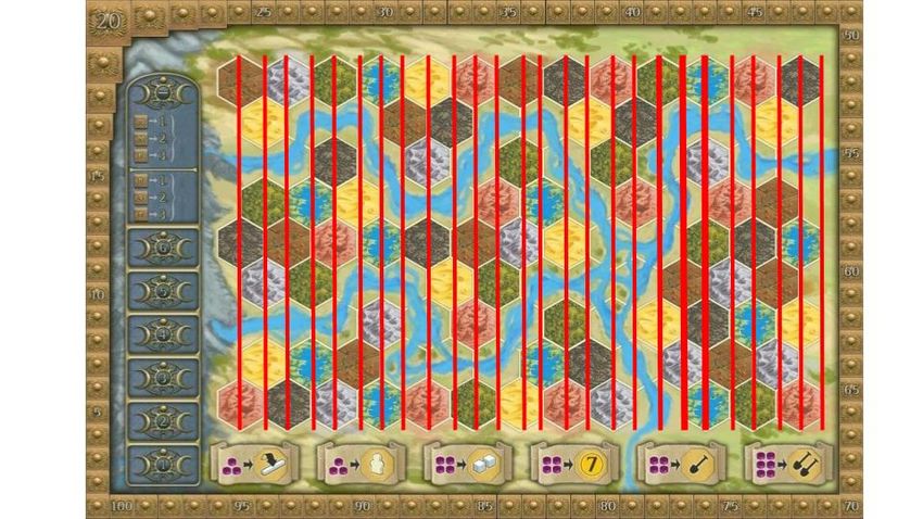
2.2. Alpha Zero for TM                                                (a) The initial DQN approach for Atari games had
                                                                          an output action space of dimension 18 (though
    In this section, we describe the main methods we use for
                                                                          some games had only 4 possible actions, the
training our agent. In particular, we place heavy emphasis
                                                                          maximum number of actions was 18 and this was
on the methods described by AlphaGo[3], AlphaGoZero,
                                                                          represented simply as a 18-dimensional vector
[5], and AlphaZero [4] with pertinent modifications made
                                                                          representing a softmax probability distribution).
for our specific problem domain.
    Our main method will be a modification of the Alpha               (b) For Go, the output actions space was similarly
Zero [4] algorithm which was described in detail. We chose                a 19 × 19 + 1 probability distribution over the
this algorithm over the methods described for Alpha Go [3]                locations on which to place a stone.
for two main reasons:                                                 (c) Even for Chess and Shogi, the action space sim-
                                                                          ilarly consisted of all legal destinations of all
 1. The Alpha Zero algorithm is a zero-knowledge rein-
                                                                          player’s pieces on the board. While this is very
    forcement learning algorithm. This is well-suited for
                                                                          expansive and more similar to what we expect
    our purposes, given that we can perfectly simulate
                                                                          for TM, TM nonetheless has additional complex-
    game-play.
                                                                          ity in that some actions are inherently hierarchi-
 2. The Alpha Zero algorithm is a simplification over the                 cal. You must first decide if you want to build,
    dual-network architecture used for AlphaGo.                           then decided where to build, and finally decide
                                                                          what to build. This involves defining an output
  As such, our goal is to demonstrate and develop a slightly              actions-space which is significantly more com-
modified general-purpose reinforcement learning algorithm                 plex than anything we’ve seen in the literature.
which can achieve super-human performance tabula-rasa on                  For comparison, in [4] the output space consists
TM.                                                                       of a stack of planes of 8 × 8 × 73. Each of the
                                                                          64 positions identifies a piece to be moved, with
2.2.1   TM Specific Challenges                                            the 73 associated layers identifying exactly how
                                                                          the piece will be moved. As can be seen, this is
We first introduce some of the TM-specific challenges our                 essentially a two-level decision tree (select piece
algorithm must overcome.                                                  followed by selecting how to move the piece). In
                                                                          TM, the action-space is far more varied.
 1. Unlike the game of Go, the rules of TM are not trans-
    lationally invariant. The rules of TM are position-          5. The next challenge is that TM is not a binary win-lose
    dependent – the most obvious way of seeing this is              situation, as is the case in Go. Instead, we must seek
    that each terrain-tile and patterns of terrains are dif-        to maximize our score relative to other players. Ad-
    ferent, making certain actions impossible from certain          ditionally, in TM, there is always the possibility of a
    positions (or extremely costly). This is not particularly       tie.
    well-suited for the weight-sharing structure of Convo-
    lutional Neural Networks.                                    6. Another challenge present in TM not present in other
                                                                    stated games is the fact that there exist a limited num-
 2. Unlike the game of Go, the rules for TM are asymmet-            ber of resources in the game. Each player has a limited
    ric. We can, again, trivially see this by noting that the       number of workers/priests/coin with which a sequence
    board game board itself 7 has little symmetry.                  of actions must be selected.
 3. The game-board is not easily quantized to exploit po-        7. Furthermore, TM is now a multi-player game (not two-
    sitional advantages. Unlike games where the Alp-                player). For our purposes, however, we leave exploring
    haZero algorithm has been previously applied (such as           this problem to later research. We focus exclusively
    Go/Shogi/Chess), the TM map is not rectangular. In              on a game between two fixed factions (Engineers and
    fact, each “position” has 6 neighbors, which is not eas-        Halflings).
    ily representable in matrix form for CNNs.
                                                                2.3. Input Representation
 4. The action space is significantly more complex and hi-
    erarchical, with multiple possible “mini”-games being          Unless otherwise specified, we leave the training and
    played. Unlike other games where similar approaches         search algorithm large unmodified from those presented in
    have been applied, this action-space is extremely com-      [4] and [5]. We will described the algorithm, nonetheless,
    plex. To see this, we detail the action-spaces for other    in detail in subsequent sections. For now, we focus on pre-
    games below.                                                sented the input representation of our game state.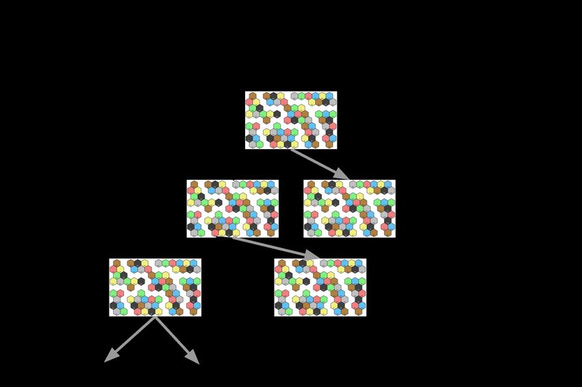
2.3.1   The Game Board                                             2.3.2   Player Representation and Resource Limitations
                                                                   We now introduce another particularity of TM, which is the
We begin by noting that the TM GameBoard 7 is naturally            fact that each player has a different amount of resources
represented as 13 × 9 hexagonal grid. As mentioned in the          which must be handled with care. This is something which
challenges section, this presents a unique problem since for       is not treated in other games, since the resource limitation
each intuitive “tile“, we have 6 rather than the the 4 (as in      does not exist in Go, Chess, or Shogi (other than those fully
Go, Chess, and Shogi). Furthermore, unlike chess where             encoded by the state of the board).
a natural dilation of the convolution will cover additional            With that in-mind, we move to the task of encoding each
tangent spots equally (expanding to 8), the hexagonal nature       player. To be fully generic, we scale this representation with
makes TM particularly interesting.                                 the number of players playing the game, in our case, P = 2.
    However, a particular peculiarity of TM is that we can             To do this, for each player, we add constant layers spec-
think of each “row” of tiles as being shifted by “half” a          ifying: (1) number of workers, (2) number of priests, (3)
tile, thereby becoming “neighbors”. With this approach, we         number of coins, (4) power in bowl I, (5) power in bowl
chose to instead represent the TM board as a 9 × 26 grid,          II, (6) power in bowl III, (7) the cost to terraform, (8) ship-
where each tile is horizontally doubled. Our terrain rep-          ping distance, (9-12) positions in each of the 4 cult tracks,
resentation of the map then begins as a 9 × 26 × 8 stack           (13-17) number of building built of each type, (18) cur-
of layers. Each layer is a binary encoding of the terrain-         rent score, (19) next round worker income, (20) next round
type for each tile. The 7 main types are {PLAIN, SWAMP,            priest income, (21) next round coin income, (22) next round
LAKE, FOREST, MOUNTAIN, WASTELAND, DESERT                          power income, (23) number of available bridges. This gives
}. It as a possible action to “terra-form“ any of these tiles      us a total of 23P additional layers required to specify infor-
into any of the other available tiles, therefore why we must       mation about the player resources.
maintain all 7 of them as part of our configuration. The 8-            Next, we consider representing the location of bridges.
th layer actually remains constant throughout the game, as         We add P layers, each corresponding to each player, in a
this layer represents the water-ways and cannot be modified.       fixed order. The each layer is a bit representing the exis-
Note that even-row (B, D, F, H) are padded at columns 0            tence/absence of a bridge at a particular location. This gives
and 25 with WATER tiles.                                           us 24P layers.
                                                                       We’ve already considered the positions of the player in
    The next feature which we tackle is the representation
                                                                   the cult-track. The only thing left is the tiles which the
of the structures which can be built on each terrain tile.
                                                                   player may have. We add 9 + 10 + 5 layers to each player.
As part of the rules of TM, a structure can only exists
                                                                   The first 9 specify which bonus card the player currently
on a terrain which corresponds to it’s player’s terrain. As
                                                                   holds. The next 10 specify which favor tiles the player cur-
such, for each tile we only need to consider the 5 possi-
                                                                   rently owns. And the last 5 specify how many town tiles
ble structures, {DWELLING, TRADING POST, SANC-
                                                                   of each type the player currently holds. This gives use an
TUARY, TEMPLE, STRONGHOLD }. We encode these
                                                                   additional 24P layers.
as an additional five-layers in our grid. Our representation
                                                                       We end with a complete stack of dimension 9×26×24P
is now a 9 × 26 × 13 stack.
                                                                   to represent P players.
   We now proceed to add a set of constant layers. First, to
represent each of the 5 special-actions, we add 6-constant         2.3.3   Putting it All Together
layers which will be either 0 or 1 signifying whether a par-
ticular action is available (0) or take (1). This gives us a       Finally, we add 14 layers to specify which of the 14 possible
9 × 26 × 19 representation.                                        factions the neural network should play as. This gives us an
                                                                   input representation of size 9×26×(48P +110). See Table
   To represent the scoring tiles (of which there are 8), we
                                                                   1 which places this into context. In our case, this becomes
add 8×6 constant layers (either all 1 or all 0) indicating their
                                                                   9 × 26 × 206.
presence in each of the 6 rounds. This gives us a 9×26×75
stack.                                                             2.4. Action Space Representation
   For favor tiles, there are 12 distinct favor tiles. We add 12       Terra Mystica is a complex game, where actions are sig-
layers each specifying the number of favor tiles remaining.        nificantly varied. In fact, it is not immediately obvious how
This gives use 9 × 26 × 87.                                        to even represent all of the possible actions. We provide a
   For the bonus tiles, we add 9 constant layers. These 9          brief overview here of our approach.
layers specify which favor tiles were selected for this game           In general, there are 8 possible actions in TM which are,
(only P + 3 cards are ever in play). This gives us a game-         generally speaking, quite distinct. In general, we output all
board representation which is of size 9 × 26 × 96                  possible actions and assign a probability. Illegal actions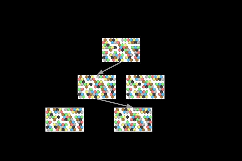
Domain             Input Dimensions        Total Size                 four possible cults. Additionally, the player must de-
 Atari 2600         84 x 84 x 4             28,224                     termine if he wants to send his priest to advance 3, 2 or
 Go                 19 x 19 x 17            6,137                      1 spaces – some of which maybe illegal moves. We can
 Chess              8 x 8 x 119             7,616                      represent this simply as a 4 × 3 vector of probabilities.
 Shogi              9 x 9 x 362             29,322
                                                                    6. Take a Board Power Action: There are 6 available
 Terra Mystica      9 x 26 x 206            48,204
                                                                       power actions on the board. We represent this as a 6×1
 ImageNet           224x224x1               50,176
                                                                       vector indicating which power action the player wishes
Table 1. Comparison of input sizes for different domain of both
games. For reference, typical CNN domain of ImageNet is also
                                                                       to take. Actions can only be take once per round.
included.                                                           7. Take a Special Action: There are multiple possible
                                                                       “special“ actions a player may choose to take. For ex-
are removed by setting their probabilities to zero and re-             ample, there’s a (1) spade bonus tile, (2) cult favor tile
normalizing the remaining actions. Actions are considered              as well as special action allowed by the faction (3). As
legal as long as they can be legally performed during that             such, we output a 3 × 1 vector in this case for each of
turn (ie, a player can and will burn power/workers/etc. in             the above mentioned actions, many of which may be
order to perform the required action. We could technically             illegal.
add additional actios for each of this possibilities, but this
                                                                    8. Pass: The player may chose to pass. If the first to pass,
vastly increases the complexity.
                                                                       the player will become the first to go next round. For
 1. Terra Form and Build: This action consists of (1) se-              this action, the player must also chose which bonus tile
    lecting a location (2) selecting a terrain to terraform to         to take. There are 9 possible bonus tiles (some which
    (if any) and (3) optionally selecting to build. We can             won’t be available, either because they were never in
    represent this process as a vector of size 9×13×(7×2).             play or because the other players have taken them). As
    The 9 × 13 is selecting a location, while the first 7 lay-         such, we represent this action by a 9 × 1 vector.
    ers the probability of terraforming into one of the 7           9. Miscellaneous: At any point during game-play for this
    terrains and not building, and the last 7 the probability          player, it may become the case that a town is founded.
    of terraforming into each of the 7 terrains and building.          For each player round, we also output a 5 × 1 vector of
 2. Advancing on the Shipping Track: The player may                    probabilities specifying which town tile to take in the
    choose to advance on the shipping track. This consists             even this has occurred. These probabilities are normal-
    of a single additional value encoding the probability of           ized independently of the other actions, as they are not
    advancement.                                                       exclusive, though most of the time they will be ignored
                                                                       since towns are founded relatively rarely (two or three
 3. : Lowering Spade Exchange Rate: The player may                     times per game).
    choose to advance on the spade track. This consists
    of a single additional value encoding the probability of      2.4.1   Concluding Remarks for Action Space Represen-
    choosing to advance on the spade track.                               tation
 4. Upgrading a Structure: This action consists of (1) se-        As described above, this leads to a relatively complex
    lecting a location, (2) selecting which structure to up-      action-space representation. In fact, we’ll end-up outputting
    grade to. Depending on the location and existing struc-       a 9×13×18+4×3+20+5 We summarize the action-space
    ture, some actions may be illegal. We can represent           representation in Table 2 and provide a few other methods
    this process as a vector of size 9 × 13 × 4 specifying        fore reference.
    which location as well as the requested upgrade to the
    structure (DWELLING to TRADING POST, TRAD-                     Domain              Input Dimensions            Total Size
    ING POST to STRONG HOLD, TRADING POST to                       Atari 2600          18 x 1                      18
    TEMPLE, or TEMPLE to SANCTUARY).                               Go                  19 x 19 + 1                 362
     Note that when a structure is built, it’s possible for the    Chess               8 x 8 x 73                  4,672
     opponents to trade victory points for power. While this       Shogi               9 x 9 x 139                 11,259
     is an interesting aspect of the game, we ignore for our       Terra Mystica       9 x 13 x 18 + 4x3 + 25      2,143
     purposes and assume players will never chose to take          ImageNet            1000x1                      1000
     additional power.                                            Table 2. Comparison of action space sizes for different domain of
                                                                  both games. For ImageNet, we consider the class-distribution the
 5. Send A Priest to the Order of A Cult: In this action,         actions-space
    the player choose to send his or her priest to one of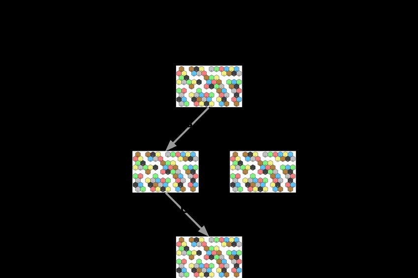
2.5. Deep Q-Learning with MCTS Algorithm and
      Modifications
   In this section, we present our main algorithm and the
modifications we’ve made so-far to make it better suited for
our state-space and action-space. We describe in detail the
algorithm for completeness, despite the algorithm remain-
ing mostly the same as that used in [4] and presented in
detail in [5].

2.5.1   Major Modifications
The main modifications to the algorithm are mostly per-
formed on the architecture of the neural network.                Figure 1. Monte Carlo Tree Search: Selection Phase. During this
                                                                 phase, starting from the root node, the algorithm selects the op-
 1. We extend the concept of introduced in [5] of “dual”         timal path until reaching an un-expanded leaf node. In the case
    heads to “multi-head“ thereby providing us with mul-         above, we select left action, then the right action, reaching a new,
    tiple differing final processing steps.                      un-expanded board state.

 2. We modify the output and input dimensions accord-
    ingly.                                                             while seen(S):
                                                                           max_u, best_a = -INF, -1
2.5.2   Overview of Approach                                               for a in Actions(S) :
                                                                               u = Q(s,a) + c*P(s,a)
We make use of a deep neural network (architecture de-                             *sqrt(visit_count(s)))
scribed in Section 2.5.5) (p, m, v) = fθ (s) with parame-                          /(1+action_count(s,a))
ters θ, state-representations s, as described in Section 2.3,                  if u>max_u:
output action-space textbf p, as described in Section 2.4,                         max_u = u
additional action-information as m as described in Section                         best_a = a
2.4.1, and a scalar value v that estimates the expected output         s = Successor(s, best_a)
z from position s v ≈ E[z | s]. The values from this neu-              v = search(sp, game, nnet)
ral network are then used to guide MCTS, and the resulting
move-probabilities and game output are used to iteratively           From above, we can see that as a sub-routing of search
update the weights for the network.                              we have the ‘Expand‘ algorithm. The expansion algorithm
                                                                 is used to initialize non-terminal, unseen states of the game
                                                                 S as follow.
2.5.3   Monte Carlo Tree Search
We provide a brief overview of the MCTS algorithm used.          def Expand(s):
We assume some familiarity with how MCTS works. In                   v, p = NN(s)
general, there are three phases which need to be considered.         InitializeCounts(s)
For any given state St which we call the root-state (this is         StoreP(s, p)
the current state of gameplay), the algorithm simulates 800          return v
iterations of gameplay. We note that AlphaGoZero [5] does
                                                                 Where ‘InitializeCounts‘ simply initializes the counts for
1600 iterations and AlphaZero does [4] also does 800.
                                                                 the new node (1 visit, 0 for each action). We also initialize
    At each node, we perform a search until a leaf-node is
                                                                 all Q(s, a) = 0 and store the values predicted by our N N .
found. A leaf-node is a game-state which has never-been
                                                                 Intuitively, we’ve now expanded the depth of our search
encountered before. The search algorithm is relatively sim-
                                                                 tree, as illustrated in Figure 2.
ple, as shown below and as illustrated in Figure 1. Note that
                                                                     After the termination of the simulation (which ended ei-
the algorithm plays for the best possible move, with some
                                                                 ther with an estimated v by the NN or an actually R), we
bias given to moves with low-visit counts.
                                                                 back-propagate the result by updating the corresponding
                                                                 Q(s, a) values using the formula:
def Search(s):
    if IsEnd(s): return R                                                           Q(s, a) = V (Succ(s, a))
    if IsLeaf(s): return Expand(s)
                                                                 This is outlined in Figure 3.
Figure 4. Detailed diagram of the multi-headed architecture ex-
plored for the game of Terra Mystica.
information (T = 1), both for computational efficiency and
Figure 2. Monte Carlo Tree Search: Expansion Phase. During
due to the fact that the game is fully encoded with the cur-
this phase, a leaf-node is “expanded”. This is where the neural rent state.
network comes in. At the leaf-node, we process the state SL to The input features st are processed by a residual tower
retrieve p, v = fθ (SL ) which consists of a single convolution block followed by
, which is a vector of probabilities for the actions that are 19 residual blocks, as per [5]. The first convolution block
possible and a value function. consists of 256 filters of kernel size 3×3 with stride 1, batch
normalization, and a ReLU non-linearity.
Figure 3. Monte Carlo Tree Search: Back-propagation Phase. Dur-
ing this phase, we use the value v estimated at the leaf-node and
propagate this information back-up the tree (along the path-taken)
to update the stored Q(s, a) values.
Figure 5. Architecture Diagram for shared processing of the state
2.5.4 Neural Network Training space features. An initial convolution block is used to standard-
ize the number of features, which is then followed by 18 residual
The training can be summarized relatively straightfor- blocks.
wardly. We batch N (with N = 128) tuples (s, p, v) and use
this to train, with the loss presented in AlphaZero [4]. We Each residual block applies the following modules, in
use c = 1 to for our training. We perform back-propagation sequence, to its input. A convolution of 256 filters of ker-
with this batch of data, and continue our games of self-play nel size 3 × 3 with stride 1, batch-normalization, and a
using the newly updated neural network. This is all per- ReLU non-linearity, followed by a second convolution of
formed synchronously. 256 filters of kernel size 3 × 3 with stride 1, and batch-
normalization. The input is then added to this, a ReLu ap-
2.5.5 Neural Network Architecture plied, and the final output taken as input for the next block.
See Figure 5 for a reference.
We first describe the architecture of our neural network. For The output of the residual tower is passed into multiple
brief overview, see Figure 4. The input is a 9 × 26 × 206 separate ’heads’ for computing the policy, value, and mis-
image stack as described in Section 2.3.3. Note that un- cellaneous information. The heads in charge of computing
like other games, our representation includes no temporal- the policy apply the following modules, which we guess atgiven that the AlphaZero Paper [4] does not discuss in detail 3.1. Baselines
how the heads are modified to handle the final values. See
Figure 6 for an overview diagram. For the base-lines, we compare the final scores achieved
by existing AI agents. We see their results in Table 4. The
results demonstrate that current AIs are fairly capable at
scoring highly during games of self-play.
Simulated Self-Play Average Scores - AI
Faction Average Score Sampled Games
Halfing 92.21 1000
Engineers 77.12 1000
Table 3. Self-play easy AI agent: AI Level5 from [6]
3.2. Oracle
A second comparison, showing in Table 4, demonstrates
the skill we would expect to achieve. These are the average
Figure 6. Details on multi-headed architecture for Neural Network. scores of the best human players, averaged over online data.
The final output state of the residual tower is fed into two paths. (1)
On the left is the policy network. (2) On the right is the value esti-
mator. The policy network is further split into two, for computing Average Human Score (2p)
two disjoint distributions over the action space, each normalized Faction Average Score Sampled Games
independently. Halfling 133.32 2227
Engineers 127.72 1543
Table 4. Average human scores by faction for a two-player TM
For the policy, we have one head that applies a convolu- games online.
tion of 64 filters with kernel size 2×2 with stride 2 along the
horizontal direction, reducing our map to 9 × 13 × 64. This
convolution is followed by batch normalization, a ReLU 3.3. AlphaTM
non-linearity.
We then split this head into two further heads. We then The results for AlphaTM are presented below. Training
apply an FC layer which outputs a vector of 9×13×18+32 appears to not have taken place, at least not with the archi-
which we interpret as discussed in Section 2.4, represent- tecture and number of iterations which we executed. The AI
ing the mutually exclusive possible actions that a player can still appears to play randomly, specially at later, and more
take. crucial, stages of the game. See Table 5.
For the second part, we apply a further convolution with
1 filter of size 1×1, reducing our input to 9×13. This is fol- Simulated Self-Play Average Scores - AlphaTM
lowed by a batch-normalization layer followed by a ReLU. Faction Average Score Training Iterations
We then apply a FC layer further producing a probability Halfing 32.11 10,000
distribution over a 5 × 1 vector. Engineers 34.12 10,000
Table 5. Our Self-Play AI after 10,000 training iterations, with
For the value head, we apply a convolution of 32 filters average score over final 1000 games.
of kernel size 1 × 1 with stride 1 to the, followed by batch
normalization and a ReLU unit. We follow this with an FC
Overall, we summarize:
to 264 units, a ReLU, another FC to a scalar, and a tanh-
nonlinearity to output a scalar in the range [−1, 1].
• The AI plays poorly in early stages of the game, though
it seems to learn to build structures adjacent to other
3. Experimental Results players.
Given the complexity of the problem we’re facing, the • As the game progresses, the actions of the agent are
majority of the work has been spent developing the re- indistinguishable from random. A cursory analysis of
inforcement learning pipeline with an implementation of π reveals these states are basically random. It appears
MCTS. The pipeline appears to not train well, even after that the AI is not learning to generalize, or has simple
multiple games of self-play. not played sufficient games.4. Future Work
Given the poor results from the experiments above, many
avenues exists for future work. In particular, we propose a
few extensions to the above approach below.
4.1. Generalizing to Multi-Player Game
In the general context, the reinforcement learning
pipeline that performed the best (with some semblance of
learning) is the one where the game was presented as a zero-
sum two-player game explicitly (I win, you lose). While
the neural network architecture presented can readily gen-
eralize to more players, the theory behind the learning algo-
rithm will no-longer hold. The game is no longer zero-sum.
4.2. New Architectures and Improvements
Another area of future work is experimenting with fur-
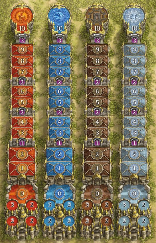
ther architectures and general improvement, with possible Figure 8. The Terra Mystica Cult Track
hyper parameter tuning.
5. Appendices
Figure 9. The Terra Mystica Board Representation
Y. Chen, T. Lillicrap, F. Hui, L. Sifre, G. van den Driessche,
T. Graepel, and D. Hassabis. Mastering the game of go with-
out human knowledge. Nature, 550:354 EP –, Oct 2017. Ar-
ticle. 1, 2, 3, 6, 7
Figure 7. The Terra Mystica Game Board and Its Representation [6] tmai. Terra mystic ai implementations, 2018. 8
References
[1] BoardGeek. Terra mystica: Statistics, 2011. 1
[2] M. LLC. Terra mystica: Rule book, 2010. 1
[3] D. Silver, A. Huang, C. J. Maddison, A. Guez, L. Sifre,
G. van den Driessche, J. Schrittwieser, I. Antonoglou, V. Pan-
neershelvam, M. Lanctot, S. Dieleman, D. Grewe, J. Nham,
N. Kalchbrenner, I. Sutskever, T. Lillicrap, M. Leach,
K. Kavukcuoglu, T. Graepel, and D. Hassabis. Mastering the
game of go with deep neural networks and tree search. Nature,
529:484 EP –, Jan 2016. Article. 1, 2, 3
[4] D. Silver, T. Hubert, J. Schrittwieser, I. Antonoglou, M. Lai,
A. Guez, M. Lanctot, L. Sifre, D. Kumaran, T. Graepel, T. P.
Lillicrap, K. Simonyan, and D. Hassabis. Mastering chess
and shogi by self-play with a general reinforcement learning
algorithm. CoRR, abs/1712.01815, 2017. 1, 2, 3, 6, 7, 8
[5] D. Silver, J. Schrittwieser, K. Simonyan, I. Antonoglou,
A. Huang, A. Guez, T. Hubert, L. Baker, M. Lai, A. Bolton,You can also read