Deep Reinforcement Learning with Population-Coded Spiking Neural Network for Continuous Control
←
→
Page content transcription
If your browser does not render page correctly, please read the page content below
Deep Reinforcement Learning with Population-Coded
                                           Spiking Neural Network for Continuous Control
                                                Guangzhi Tang, Neelesh Kumar, Raymond Yoo, and Konstantinos P. Michmizos
                                                                      Department of Computer Science
                                                                            Rutgers University
                                                          {gt235, nk525, rby6, michmizos}@cs.rutgers.edu
arXiv:2010.09635v1 [cs.NE] 19 Oct 2020

                                                  Abstract: The energy-efficient control of mobile robots has become crucial
                                                  as the complexity of their real-world applications increasingly involves high-
                                                  dimensional observation and action spaces, which cannot be offset by their limited
                                                  on-board resources. An emerging non-Von Neumann model of intelligence, where
                                                  spiking neural networks (SNNs) are executed on neuromorphic processors, is now
                                                  considered as an energy-efficient and robust alternative to the state-of-the-art real-
                                                  time robotic controllers for low dimensional control tasks. The challenge now for
                                                  this new computing paradigm is to scale so that it can keep up with real-world
                                                  applications. To do so, SNNs need to overcome the inherent limitations of their
                                                  training, namely the limited ability of their spiking neurons to represent informa-
                                                  tion and the lack of effective learning algorithms. Here, we propose a population-
                                                  coded spiking actor network (PopSAN) that was trained in conjunction with a deep
                                                  critic network using deep reinforcement learning (DRL). The population coding
                                                  scheme, which is prevalent across brain networks, dramatically increased the rep-
                                                  resentation capacity of the network and the hybrid learning combined the training
                                                  advantages of deep networks with the energy-efficient inference of spiking net-
                                                  works. To show that our approach can be used for general-purpose spike-based
                                                  reinforcement learning, we demonstrated its integration with a wide spectrum of
                                                  policy-gradient based DRL methods covering both on-policy and off-policy DRL
                                                  algorithms. We deployed the trained PopSAN on Intel’s Loihi neuromorphic chip
                                                  and benchmarked our method against the mainstream DRL algorithms for con-
                                                  tinuous control. To allow for a fair comparison among all methods, we validated
                                                  them on OpenAI gym tasks. Our Loihi-run PopSAN consumed 140 times less en-
                                                  ergy per inference when compared against the deep actor network on Jetson TX2,
                                                  and achieved the same level of performance. Our results demonstrate the over-
                                                  all efficiency of neuromorphic controllers and suggest the hybrid reinforcement
                                                  learning approach as an alternative to deep learning, when both energy-efficiency
                                                  and robustness are important.

                                                  Keywords: Spiking neural networks, Deep reinforcement learning, Energy-
                                                  efficient continuous control

                                         1   Introduction
                                         Mobile robots with continuous high-dimensional observation and action spaces are increasingly be-
                                         ing deployed to solve complex real-world tasks. Given their limited on-board energy resources, there
                                         is an unmet need to design energy-efficient solutions for the continuous control of these autonomous
                                         robots. Deep reinforcement learning (DRL) methods based on policy-gradient have been successful
                                         in learning optimal control policies for complex tasks [1, 2]; However, their optimality comes at the
                                         cost of high energy consumption, rendering them ill-suited for several applications [3].
                                         An energy-efficient alternative to deep networks is provided by spiking neural networks (SNNs)
                                         deployed on neuromorphic processors. In this emerging neuromorphic computing paradigm, where
                                         memory and computation are tightly integrated, neurons perform asynchronous, event-based com-
                                         putations [4]. Mounting studies are suggesting SNNs as low-energy solutions for several real-world

                                         4th Conference on Robot Learning (CoRL 2020), Cambridge MA, USA.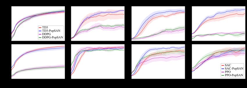
robotic problems [5, 6, 7]. For robotic control, SNN approaches are typically based on reward-
modulated local learning rules [8, 9] that perform well in low-dimensional tasks but often fail in com-
plex problems, where optimization becomes difficult in the absence of a global loss function [10].
Recently, [11] proposed a policy gradient-based algorithm to train an SNN for learning stochastic
policies. However, the algorithm operates over a discrete action space, with a rather limited use on
high-dimensional continuous control problems.
To address the limitations of SNN in solving high-dimensional continuous control problems, one
approach is to combine the energy-efficiency of SNN with the optimality of DRL. To this end, a
popular SNN construction method is to directly convert a trained deep neural network (DNN) into
an SNN using weight and threshold balancing [12]. The main problems with this approach are that it
often results to a spiking network with an inferior performance to the corresponding DNN, and also
requires large timesteps for inference that dramatically increases the energy cost [13]. To overcome
this, a recent work proposed a hybrid learning algorithm where an SNN with rate-coded inputs is
trained using DRL to learn optimal control policies for mapless navigation of a mobile robot in a
static environment [14]. However, this method suffers in complex high-dimensional tasks where
the optimality of the control policy highly depends on the encoding precision of individual spiking
neurons that have limited representation ability [15]. The practicality of this solution becomes even
less when a small inference timestep is used for higher energy-efficiency, since this is expected to
further reduce the representation ability of the neurons as they encode data using their firing rate.
Interestingly, abstracting away the brain’s topology and its computational principles has recently
given rise to the design of SNNs that exhibit human-like behavior [16] and improved perfor-
mance [17]. A key attribute in the brain associated with efficient computation is the use of pop-
ulations of neurons to represent information, from sensory stimuli to output signals, where each
neuron in a population has a receptive field that captures part of the encoded signal [18]. Indeed,
initial studies on the population coding scheme have demonstrated its ability to better represent
the stimuli [19], which led to recent successes in training SNNs for complex high-dimensional su-
pervised learning tasks [20, 21]. The demonstrated effectiveness of the population coding opens
up prospects for developing efficient population-coded SNNs that can learn optimal solutions for
high-dimensional continuous control tasks.
In this paper, we propose a population-coded spiking actor network (PopSAN) that is trained using
DRL algorithms to learn energy-efficient solutions for continuous control problems1 . At the core of
our PopSAN lies its ability to encode each dimension of the observation and action spaces in indi-
vidual neuron populations with learnable receptive fields, effectively increasing the representation
capacity of the network. Since different control tasks require specialized DRL solutions [22], we in-
tegrated our PopSAN with both on-policy and off-policy DRL algorithms, in particular, DDPG [23],
TD3 [24], SAC [25], and PPO [26], thereby demonstrating its applicability to a wide spectrum of
policy-gradient based DRL algorithms. We deployed the trained PopSAN on Intel’s Loihi neuromor-
phic processor and evaluated our method on OpenAI gym tasks with rich and unstable dynamics that
are used in benchmarking continuous control algorithms. We compared our method on its rewards
gained and energy consumption against the mainstream DRL algorithms. Our Loihi-run PopSAN
consumed 140 times less energy per inference when compared against the deep actor network on
Jetson TX2, while also achieving the same level of performance. These results introduce the DRL
algorithms to the spiking domain, scaling them as neuromorphic solutions to reinforcement learning
tasks where energy efficiency matters.

2         Methods

2.1        Population-coded Spiking Actor Network (PopSAN) embedded into DRL algorithms

We propose a population-coded spiking actor network (PopSAN) that is trained in conjunction with
a deep critic network using the DRL algorithms. During training, the PopSAN generated an action
a ∈ RN for a given observation, s, and the deep critic network predicted the associated state-
value V (s) or action-value Q(s, a), which in turn optimized the PopSAN, in accordance with a
chosen DRL method (Fig. 1). The encoder module in the PopSAN encoded each dimension of the
observation into the activity of an individual neuron population. During forward propagation, the
      1
          Code available at https://github.com/combra-lab/pop-spiking-deep-rl

                                                          2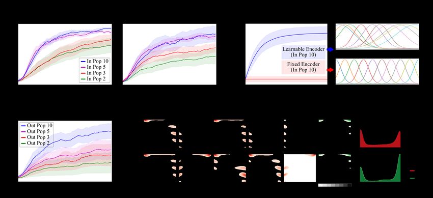
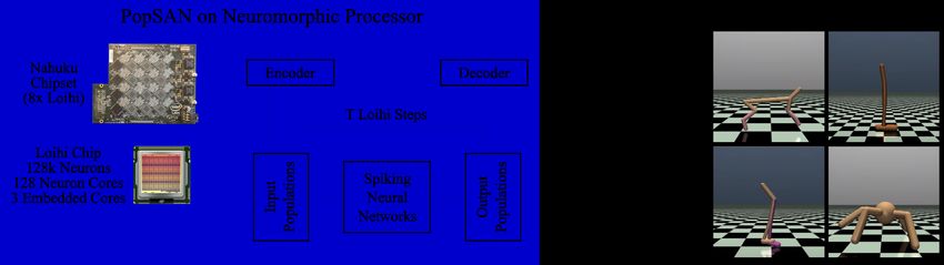
Figure 1: Population-coded spiking actor network (PopSAN) was trained in conjunction with a deep
critic network using the DRL algorithms. Neurons in the input populations encoded each observation
dimension and drove a multi-layered and fully connected SNN. At the end of forward timesteps, the
activities of each output population was decoded into its corresponding action dimension.

input populations drove a multi-layered and fully-connected SNN to produce activities of output
populations which were then decoded into their corresponding action dimensions at the end of every
T timesteps (Algorithm 1).
To build the SNN, we used the current-based leaky-integrate-and-fire (LIF) model of a spiking neu-
ron. The dynamics of the LIF neurons are governed by a 2 step model as described in Algorithm 1:
i) integrating the presynaptic spikes o into current c; and ii) integrating the current c into membrane
voltage v; dc and dv are the current and voltage decay factors. Subsequently, the neuron fires a
spike if its membrane potential exceeds a threshold. We used the hard-reset model where the mem-
brane potential is reset to rest potential upon spiking. The resultant spikes are transmitted to the
post-synaptic neurons at the same inference timestep, assuming zero propagation delay.

 Algorithm 1: Forward propagation through PopSAN
  Randomly initialize weight matrices W and biases b for each SNN layer;
  Initialize encoding means µ and standard deviations σ for all input populations;
  Randomly initialize decoding weight vectors Wd and bias bd for each action dimension;
  N -dimensional observation, s;
  Spikes from input populations generated by the encoder module : X = Encoder(s, µ, σ);
  for t=1,...,T do
       Spikes from input populations at timestep t: o(t)(0) = X(t) ;
       for k=1,...,K do
           Update LIF neurons in layer k at timestep t based on spikes from layer k − 1:
           c(t)(k) = dc · c(t−1)(k) + W(k) o(t)(k−1) + b(k) ;
           v(t)(k) = dv · v(t−1)(k) · (1 − o(t−1)(k) ) + c(t)(k) ;
           o(t)(k) = T hreshold(v(t)(k) );
       end
  end
  M -dimensional action a generated by the decoder module:
                                                      PT
  Sum up the spikes of output populations: sc = t=1 o(t)(K) ;
  for i=1,...,M do
       Compute firing rates of the ith output population : fr(i) = sc(i) / T ;
                                                    (i)            (i)
       Compute ith dimension of action: ai = Wd · fr(i) + bd ;
  end

Our PopSAN is functionally equivalent to a deep actor network and can be integrated with any
actor-critic based DRL algorithm. Specifically, we integrated the PopSAN with both on-policy and
off-policy DRL algorithms, namely DDPG [23], TD3 [24], SAC [25], and PPO [26], as follows: For
DDPG and TD3, we trained the PopSAN to predict the action for which the trained critic network

                                                  3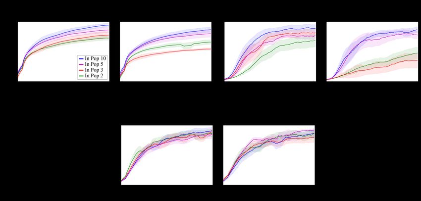
generated the maximum action-value. For SAC, we trained the PopSAN to predict the mean of the
stochastic action distribution, and a deep network to predict its standard deviation. This was done
by minimizing the distance between the probability of the action sampled from the predicted distri-
bution and the predicted action-value generated by the trained critic network. For PPO, the PopSAN
was trained to predict the mean of the action distribution by optimizing the clipped surrogate loss.

2.2   Population encoding and decoding in PopSAN

We encoded each dimension of the observation and action space into the activities of individual input
and output population of spiking neurons. The encoder module converted the continuous observation
into spikes in the input populations, and the decoder module decoded the output population activities
into real-valued actions.
For the ith dimension of the N -dimensional observation, si , i ∈ {1...N }, we created a population
of neurons, Ei , to encode it. Dropping the i for notational simplicity, the neurons in E had Gaussian
receptive fields (µ, σ). The µ were initialized to be evenly distributed in the space of s and σ were
preset to be large enough to ensure non-zero population activity in the entire space of s.
The encoder module computed the activity of the population E in two phases: It first transformed
the observation values into the stimulation strength for each neuron in the population, AE :
                                AE = EXP (−1/2 · ((s − µ)/σ)2 )                                          (1)
Second, the computed AE was used to generate the spikes of the neurons in E. There are two
possible ways to do this: i) Probabilistic encoding, where spikes for all the neurons were generated
at each timestep with the probabilities defined by AE ; and ii) Deterministic encoding, where the
neurons in E were simulated as one-step soft-reset IF neurons, with AE acting as the presynaptic
inputs to the neurons. The dynamics of the neurons were governed by the following equation:
                                      v(t) = v(t − 1) + AE
                                                                                                         (2)
                     ok (t) = 1 & vk (t) = vk (t) − (1 − ), if vk (t) > 1 −
where k denotes the index of a neuron in E and  is a small constant. For both types of encoders,
µ and σ are task-specific trainable parameters. In our experiments, we employed both types of
encoders for the second phase.
The output layer of the SNN comprised of populations of neurons, where a population Di repre-
sented dimension i of the M -dimensional action, ai , i ∈ {1...M }. Dropping the i for notational
simplicity, the decoder module decoded the activity of the output population, D, into its correspond-
ing real-valued action in two phases: First, after every T timesteps, the spikes of each neuron in
D were summed up to obtain the firing rate fr over T . Second, the action a was returned as the
weighted sum of the computed fr (Algorithm 1). The receptive fields of the output populations were
formed by their connection weights which were learned as part of the training.

2.3   PopSAN training

We used gradient descent to update the PopSAN parameters where the exact loss function depended
upon the chosen DRL algorithm, as explained in Section 2.1. The gradient of the loss with respect
to the computed action ∇a L was used to train the parameters of PopSAN.
The parameters for each output population i, i ∈ 1, ..., M were updated independently as follows:

                                                  (i)                                           (i)
                    ∇W(i) L = ∇ai L · Wd · fr(i)                 ,       ∇b(i) L = ∇ai L · Wd            (3)
                        d                                                  d

The SNN parameters were updated using the extended spatiotemporal backpropagation introduced
in [14]. We used the rectangular function z(v), defined in [27], to approximate the gradient of a
spike. The gradient of the loss with respect to the SNN parameters for each layer k were computed
by collecting the gradients backpropagated from all the timesteps:
                             T
                             X                                                        T
                                                                                      X
                                       (t)(k−1)
                 ∇W(k) L =         o              · ∇c(t)(k) L       ,    ∇b(k) L =         ∇c(t)(k) L   (4)
                             t=1                                                      t=1

                                                          4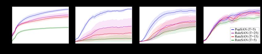
Figure 2: PopSAN deployed on Intel’s Loihi neuromorphic processor for energy-efficient and real-
time continuous control. Loihi interfaced with the continuous control task environment in real-time
using the interaction framework. Blue arrows indicate the sequence of operations inside the Loihi
chip.

Lastly, we updated the parameters independently for each input population i, i ∈ 1, ..., N as follows:

                T                                                      T
                X                             si − µ(i)               X
                                                                                           (i) (si − µ )
                                                                                                         (i) 2
    ∇µ(i) L =         ∇o(t)(0) L · AE (i) ·          2  , ∇ σ (i) L =     ∇  (t)(0) L · AE
                                                                            oi
                                                                                              ·          3     (5)
                t=1
                         i                      σ (i)                 t=1
                                                                                                   σ (i)

We updated all parameters every T timesteps. For a step-by-step analysis of the flow of gradients
during the training, we direct the readers to Section 1 of the supplementary material.

2.4    Energy-efficient continuous control with Intel’s Loihi neuromorphic chip

We deployed the trained PopSAN on Intel’s Loihi neuromorphic chip (Fig. 2). To this end, we
introduced an interaction framework that enabled Loihi to control the agents in the OpenAI gym in
real-time. To reduce the communication overhead, the first phase of the encoding (computation of
AE ) was carried out on the computer that hosted the task environment, and the second phase (spike
generation) was performed on the low-frequency x86 chip embedded on Loihi. Likewise, the first
phase of the decoding (computation of fr) was performed on the embedded chip, and the second
phase (action computation) was performed on the host computer.
We then used the layer-wise rescaling technique to map the trained PopSAN with full-precision
weights onto the low-precision loihi chip [14]. Lastly, we forced each layer in the SNN on Loihi
to start its operation one timestep after its previous layer started its operation. This was done be-
cause the postsynaptic neurons on Loihi receive the presynaptic spikes in the next timestep of their
operation, as opposed to GPUs where they are received at the same timestep.

3     Experiments and Results

The goals of our experiments were the following: i) To demonstrate the integration of PopSAN with
both on-policy and off-policy DRL algorithms by benchmarking the performance of our method
against the corresponding deep actor networks; ii) To demonstrate the need for population coding
through comparison with the state-of-the-art SNN approaches and examining the effect of learning
in neuron populations; and iii) To demonstrate PopSAN’s advantage in performing energy-efficient
and real-time continuous control when deployed on Loihi. We evaluated our method on the OpenAI
gym [28] tasks with rich and unstable dynamics that are commonly used for benchmarking continu-
ous control algorithms. To limit the effect of initialization, we trained ten models for each algorithm
corresponding to ten random seeds. Each model was trained for 1 million steps and evaluated ev-
ery 10k steps by testing it using the deterministic policy outputted by the actor. To compensate for
the effect of randomness in the tasks, we computed the average rewards over 10 episodes for each
evaluation, where each episode lasted for a maximum of 1000 execution steps.

                                                            5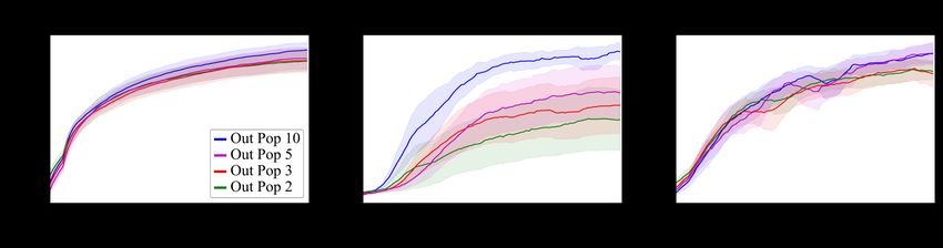
Figure 3: PopSAN trained using on-policy and off-policy DRL algorithms achieved the same level of
performance as the deep actor networks across all the environments. Figure shows the mean rewards
and half the value of standard deviation (top panel: TD3, DDPG; bottom panel: SAC, PPO). Plots
are smoothed for clarity.

3.1   Benchmarking PopSAN against mainstream DRL algorithms

We compared the performance of PopSAN trained using the on-policy and off-policy DRL algo-
rithms against the corresponding deep actor networks. Our method achieved the same level of
performance as the deep actor networks across all the tasks for all the DRL algorithms (Fig. 3),
indicating that the two approaches are functionally equivalent. The hyperparameters for training can
be found in Section 2 of the supplementary material.

3.2   Benchmarking PopSAN against other SNN design approaches

We compared our method against the following two recently suggested approaches for integrating
SNN with DRL: i) DNN to SNN conversion method (DNN-SNN) in which a deep actor network is
trained using the DRL algorithms and is converted to an SNN using weight rescaling [12]. In the
converted SNNs, the post-spike membrane potential of the LIF neurons can be set to rest potential
(hard-reset; H) or a positive potential to retain information about the previous spikes (soft-reset; S)
which demonstrated better performance in a recent study [29]. For implementation details, we direct
the readers to Section 3 of the supplementary material. ii) SAN with rate-coded inputs (RateSAN)
that uses single neuron representation to encode the inputs and the outputs and is trained using
the hybrid learning algorithm [14]. The experiments reported here were performed using the TD3
algorithm.
The two SNN approaches failed to match the performance of our method even when trained with a
value of T that was 5 times higher (Fig. 4; Table 1). This could be because both the SNN approaches
had a limited representation capacity; While the DNN-SNN method suffered from loss in precision
during conversion, the RateSAN method had an inherent limitation on the representation capacity of
individual neurons. This is further supported by the large performance decrease in the Hopper task
which has highly unstable dynamics.

3.3   Learning in neuron populations

To further demonstrate the need for population coding, we evaluated the effect of the input and out-
put neuron population size on the performance of the PopSAN trained using TD3, and investigated
how learning influenced the representation capacity of the input and output neuron populations.
First, we trained PopSAN with different input population sizes per observation dimension: 2, 3,
5, 10 while keeping the output population size fixed to 10. Fig. 5a shows that a decrease in the
input population size hurt the performance of PopSAN. To investigate the effect of learning in the
encoder, we trained PopSAN with fixed encoders in which the encoder parameters (µ, σ) remained
unchanged during training. The learnable encoder performed better than the fixed encoder (Fig.
5a) for all input population sizes. A possible reason for the superior performance of the learnable
encoder could be its ability to better separate different observations in its encoding. To justify

                                                  6
Figure 4: PopSAN (T=5) consistently performs better than RateSAN (T=5,15,25). All models were
trained using TD3 algorithm.
Table 1: Max average rewards over 10 models for PopSAN and DNN-SNN.
(T, Reset, Device) HalfCheetah Hopper Walker2d Ant
PopSAN (5, H, GPU) 10729 (σ-644) 3599 (σ-68) 4995 (σ-682) 5416 (σ-673)
PopSAN (5, H, Loihi) 10505 (σ-636) 3289 (σ-292) 4280 (σ-987) 5220 (σ-625)
DNN-SNN (5, H, GPU) 3991 (σ-925) 996 (σ-683) 391 (σ-359) -35 (σ-743)
DNN-SNN (5, S, GPU) 5256 (σ-931) 1129 (σ-879) 768 (σ-786) -7 (σ-719)
DNN-SNN (15, H, GPU) 6989 (σ-937) 1704 (σ-1215) 1804 (σ-1286) 148 (σ-793)
DNN-SNN (15, S, GPU) 9729 (σ-859) 2385 (σ-1403) 4116 (σ-724) 1634 (σ-1116)
DNN-SNN (25, H, GPU) 7913 (σ-955) 1932 (σ-1393) 2475 (σ-1318) 347 (σ-664)
DNN-SNN (25, S, GPU) 10722 (σ-806) 2523 (σ-1346) 4565 (σ-1033) 3026 (σ-1718)
this hypothesis, we computed the average L2 distance between the spike encodings of different
observations for fixed and learnable encoders. The learnable encoder resulted in an encoding that
increased the distance between the different observations (Fig. 5a), thereby suggesting that it learned
better input representations.
Next, we trained PopSAN with different output population sizes per action dimension: 2, 3, 5, 10
while keeping the input population size fixed to 10. The performance improved with the increasing
output population size (Fig. 5b). To inspect the learned action representations of the PopSAN, we
computed the receptive fields of the output population neurons by estimating the joint probability
density of the neuron activity and the predicted action values using kernel density estimation. Fig.
5b shows that PopSAN with larger population size learned redundant representations of action and
could cover a wider range of action values. This suggests that PopSAN with large output population
size can learn better action representation.
3.4 Evaluating continuous control on Loihi
To validate PopSAN’s applicability in performing energy-efficient and real-time continuous control,
we deployed it on Loihi. Our approach on Loihi exhibited high performance in terms of rewards
gained (Table 1) with only a marginal decrease when compared to PopSAN on a full-precision
GPU. We then computed the inference speed and energy consumption for the continuous control of
HalfCheetah-v3 using i) deep actor network on CPU (E5-1600), GPU (Tesla K40), embedded AI
chip (Jetson TX2- energy-efficient (Q) and high-performance (N) modes), and ii) PopSAN on Loihi
(Nahuku 8). We computed the energy cost per inference as the ratio of the dynamic power and the
number of inferences performed per second. Our PopSAN on Loihi was 140 times more energy-
efficient than the deep actor network on the low-power processor for DNNs- Jetson TX2 (Table 2),
and also had high inference speed, which enabled real-time control.
4 Discussion and Conclusion
In this paper, we presented PopSAN, a population-coded SNN, that achieved the same level of
performance as deep networks while being two orders of magnitudes more energy-efficient. The
similarity in performance was consistent when we integrated PopSAN with both on-policy and off-
policy DRL methods. This demonstrates its applicability to a wide spectrum of policy-gradient
based DRL algorithms, highlighting its use in solving several reinforcement learning tasks including
continuous control.
7Figure 5: Learning in neuron populations for PopSAN trained using TD3 for Hopper-v3. a. Learn-
ing in the input populations led to a better input representation and increase in performance. b.
Larger output populations size learned redundant and better action representations and resulted in
higher rewards. Receptive fields for each neuron in the output population corresponding to an action.
Table 2: Power performance and inference speed across hardware
Method Device Idle (W) Dynamic (W) Inf/s µJ/Inf
DNN CPU 15.51 58.93 7450 7909.86
DNN GPU 24.68 46.04 3782 12174.46
DNN TX2(N) 1.24 1.76 750 2346.71
DNN TX2(Q) 1.05 0.73 438 1670.94
PopSAN Loihi 1.084 0.003 226 11.98
The population coding scheme increased the representation capacity of the network and led to better
encodings of observations and actions. This enabled the PopSAN trained in conjunction with a deep
network to effectively learn complex high-dimensional continuous control tasks with less timesteps
for inference. While most prior works on SNNs have a predominant focus on the network design and
training [20, 27], our work demonstrates that an appropriate learnable encoding of the network inputs
and outputs with the right inductive priors can lead to a substantial increase in the performance.
The PopSAN running on Loihi was 140 times more energy-efficient on continuous control tasks than
the deep actor network running on TX2, an embedded power-efficient AI chip. This result becomes
particularly important in real-world mobile robot applications such as disaster-relief and planetary
exploration where on board resources are limited. Such applications typically rely on multimodal
sensing for robustness [30] and require high-dimensional actions for dexterity [1]. DRL methods
overcome the problem of high-dimensionality of the inputs and outputs through the use of large
networks such as a deep convolutional neural network [2]. The use of such large networks, however,
significantly increases the energy costs for control [3]. On the other hand, our proposed method can
potentially decrease the energy costs by a large factor for such applications, while further improve-
ments in energy-efficiency are expected by employing event-based sensors [31] and memristive
neuromorphic processors [32], which are much more efficient than their digital counterparts.
We showed here that the PopSAN can be successfully integrated with both on-policy and off-policy
DRL algorithms, highlighting its applicability to a wide variety of tasks that require specialized
DRL solutions [22]. This is particularly significant in real-world reinforcement learning applications
where several factors such as sample efficiency of the algorithm, stochasticity of the environment,
objectives of the reward function, and safety constraints determine which DRL algorithm would be
most appropriate for a given task [33]. Overall, our proposed spike-based solution can become a
strong alternative to deep learning for real-world reinforcement learning applications, when both
energy-efficiency and robustness are important.
8Acknowledgments
This work is supported by Intel’s NRC Grant Award.
References
[1] S. Ha, J. Kim, and K. Yamane. Automated deep reinforcement learning environment for hard-
ware of a modular legged robot. In 2018 15th International Conference on Ubiquitous Robots
(UR), pages 348–354. IEEE, 2018.
[2] Y. Zhu, R. Mottaghi, E. Kolve, J. J. Lim, A. Gupta, L. Fei-Fei, and A. Farhadi. Target-driven
visual navigation in indoor scenes using deep reinforcement learning. In 2017 IEEE interna-
tional conference on robotics and automation (ICRA), pages 3357–3364. IEEE, 2017.
[3] X. Dong, J. Huang, Y. Yang, and S. Yan. More is less: A more complicated network with less
inference complexity. In Proceedings of the IEEE Conference on Computer Vision and Pattern
Recognition, pages 5840–5848, 2017.
[4] M. Davies, N. Srinivasa, T.-H. Lin, G. Chinya, Y. Cao, S. H. Choday, G. Dimou, P. Joshi,
N. Imam, S. Jain, et al. Loihi: A neuromorphic manycore processor with on-chip learning.
IEEE Micro, 38(1):82–99, 2018.
[5] G. Tang, A. Shah, and K. P. Michmizos. Spiking neural network on neuromorphic hardware
for energy-efficient unidimensional slam. In 2019 IEEE/RSJ International Conference on In-
telligent Robots and Systems (IROS), pages 4176–4181. IEEE, 2019.
[6] T. Taunyazoz, W. Sng, H. H. See, B. Lim, J. Kuan, A. F. Ansari, B. Tee, and H. Soh. Event-
driven visual-tactile sensing and learning for robots. In Proceedings of Robotics: Science and
Systems, July 2020.
[7] C. Michaelis, A. B. Lehr, and C. Tetzlaff. Robust robotic control on the neuromorphic research
chip loihi. arXiv preprint arXiv:2008.11642, 2020.
[8] Z. Bing, C. Meschede, K. Huang, G. Chen, F. Rohrbein, M. Akl, and A. Knoll. End to end
learning of spiking neural network based on r-stdp for a lane keeping vehicle. In 2018 IEEE
International Conference on Robotics and Automation (ICRA), pages 1–8. IEEE, 2018.
[9] N. Frémaux, H. Sprekeler, and W. Gerstner. Reinforcement learning using a continuous time
actor-critic framework with spiking neurons. PLoS computational biology, 9(4), 2013.
[10] R. Legenstein, C. Naeger, and W. Maass. What can a neuron learn with spike-timing-dependent
plasticity? Neural computation, 17(11):2337–2382, 2005.
[11] B. Rosenfeld, O. Simeone, and B. Rajendran. Learning first-to-spike policies for neuromor-
phic control using policy gradients. In 2019 IEEE 20th International Workshop on Signal
Processing Advances in Wireless Communications (SPAWC), pages 1–5. IEEE, 2019.
[12] D. Patel, H. Hazan, D. J. Saunders, H. T. Siegelmann, and R. Kozma. Improved robustness of
reinforcement learning policies upon conversion to spiking neuronal network platforms applied
to atari breakout game. Neural Networks, 120:108–115, 2019.
[13] N. Rathi, G. Srinivasan, P. Panda, and K. Roy. Enabling deep spiking neural net-
works with hybrid conversion and spike timing dependent backpropagation. arXiv preprint
arXiv:2005.01807, 2020.
[14] G. Tang, N. Kumar, and K. P. Michmizos. Reinforcement co-learning of deep and spiking
neural networks for energy-efficient mapless navigation with neuromorphic hardware. 2020
IEEE/RSJ International Conference on Intelligent Robots and Systems (IROS), pages 1–8,
2020.
[15] B. B. Averbeck, P. E. Latham, and A. Pouget. Neural correlations, population coding and
computation. Nature reviews neuroscience, 7(5):358–366, 2006.
9[16] P. Balachandar and K. P. Michmizos. A spiking neural network emulating the structure of
the oculomotor system requires no learning to control a biomimetic robotic head. 8th IEEE
RAS/EMBS International Conference on Biomedical Robotics and Biomechatronics (BioRob),
pages 1–6, 2020.
[17] R. Kreiser, A. Renner, V. R. Leite, B. Serhan, C. Bartolozzi, A. Glover, and Y. Sandamirskaya.
An on-chip spiking neural network for estimation of the head pose of the icub robot. Frontiers
in Neuroscience, 14, 2020.
[18] A. P. Georgopoulos, A. B. Schwartz, and R. E. Kettner. Neuronal population coding of move-
ment direction. Science, 233(4771):1416–1419, 1986.
[19] G. Tkačik, J. S. Prentice, V. Balasubramanian, and E. Schneidman. Optimal population coding
by noisy spiking neurons. Proceedings of the National Academy of Sciences, 107(32):14419–
14424, 2010.
[20] G. Bellec, D. Salaj, A. Subramoney, R. Legenstein, and W. Maass. Long short-term memory
and learning-to-learn in networks of spiking neurons. In Advances in Neural Information
Processing Systems, pages 787–797, 2018.
[21] Z. Pan, J. Wu, M. Zhang, H. Li, and Y. Chua. Neural population coding for effective temporal
classification. In 2019 International Joint Conference on Neural Networks (IJCNN), pages
1–8. IEEE, 2019.
[22] P. Henderson, R. Islam, P. Bachman, J. Pineau, D. Precup, and D. Meger. Deep reinforcement
learning that matters. In Thirty-Second AAAI Conference on Artificial Intelligence, 2018.
[23] T. P. Lillicrap, J. J. Hunt, A. Pritzel, N. Heess, T. Erez, Y. Tassa, D. Silver, and D. Wierstra.
Continuous control with deep reinforcement learning. arXiv preprint arXiv:1509.02971, 2015.
[24] S. Fujimoto, H. Hoof, and D. Meger. Addressing function approximation error in actor-critic
methods. In International Conference on Machine Learning, pages 1587–1596, 2018.
[25] T. Haarnoja, A. Zhou, P. Abbeel, and S. Levine. Soft actor-critic: Off-policy maximum entropy
deep reinforcement learning with a stochastic actor. In International Conference on Machine
Learning, pages 1861–1870, 2018.
[26] J. Schulman, F. Wolski, P. Dhariwal, A. Radford, and O. Klimov. Proximal policy optimization
algorithms. arXiv preprint arXiv:1707.06347, 2017.
[27] Y. Wu, L. Deng, G. Li, J. Zhu, and L. Shi. Spatio-temporal backpropagation for training
high-performance spiking neural networks. Frontiers in neuroscience, 12:331, 2018.
[28] G. Brockman, V. Cheung, L. Pettersson, J. Schneider, J. Schulman, J. Tang, and W. Zaremba.
Openai gym, 2016.
[29] B. Han, G. Srinivasan, and K. Roy. Rmp-snn: Residual membrane potential neuron for en-
abling deeper high-accuracy and low-latency spiking neural network. In Proceedings of the
IEEE/CVF Conference on Computer Vision and Pattern Recognition, pages 13558–13567,
2020.
[30] G.-H. Liu, A. Siravuru, S. Prabhakar, M. Veloso, and G. Kantor. Learning end-to-end multi-
modal sensor policies for autonomous navigation. arXiv preprint arXiv:1705.10422, 2017.
[31] A. I. Maqueda, A. Loquercio, G. Gallego, N. Garcı́a, and D. Scaramuzza. Event-based vision
meets deep learning on steering prediction for self-driving cars. In Proceedings of the IEEE
Conference on Computer Vision and Pattern Recognition, pages 5419–5427, 2018.
[32] A. Ankit, A. Sengupta, P. Panda, and K. Roy. Resparc: A reconfigurable and energy-efficient
architecture with memristive crossbars for deep spiking neural networks. In Proceedings of the
54th Annual Design Automation Conference 2017, pages 1–6, 2017.
[33] G. Dulac-Arnold, D. Mankowitz, and T. Hester. Challenges of real-world reinforcement learn-
ing. arXiv preprint arXiv:1904.12901, 2019.
10Supplementary Materials: Deep Reinforcement Learning with
Population-Coded Spiking Neural Network for Continuous Control
1 PopSAN training using backpropagation
Here, we analyze the step-by-step flow of the gradients during the training of PopSAN. The gradient
of the loss with respect to the computed action, ∇a L was used to train the parameters of PopSAN.
The parameters for each output population i, i ∈ 1, ..., M were updated independently as follows:
(i)
∇fr(i) L = ∇ai L · Wd
(6)
∇W(i) L = ∇fr(i) L · fr(i) , ∇b(i) L = ∇fr(i) L
d d
The SNN parameters were updated using the extended spatiotemporal backpropagation for which
we used the rectangular function equation (7) to approximate the gradient of a spike.
1 if |v − Vth | < a
z(v) = (7)
0 otherwise
where z is the pseudo-gradient, a is the threshold window for passing the gradient.
For each timestep, t < T , the flow of the gradients through the SNN can be described as follows:
At the output population layer K, we have:
1
∇sc L = · ∇fr L , ∇o(t)(K) L = ∇sc L (8)
T
Then for each layer, k = K down to 1:
∇v(t)(k) L = z(v(t)(k) ) · ∇o(t)(k) L + dv (1 − o(t)(k) ) · ∇v(t+1)(k) L
∇c(t)(k) L = ∇v(t+1)(k) L + dc ∇c(t+1)(k) L (9)
(k)0
∇o(t)(k−1) L = W · ∇c(t)(k) L
When t = T , the gradients with respect to voltage and current do not have the second additive
term of (9) since the temporal gradients backpropagated from the future timesteps are absent. The
gradient of the loss with respect to the SNN parameters for each layer k can then be computed by
collecting the gradients backpropagated from all the timesteps:
T
X T
X
∇W(k) L = o(t)(k−1) · ∇c(t)(k) L , ∇b(k) L = ∇c(t)(k) L (10)
t=1 t=1
Lastly, we computed the gradient of the loss with respect to the parameters for each input population
i, i ∈ 1, ..., N . For simplicity, we directly backpropagated the gradient w.r.t. the neuron stimulation
strength AE regardless of whether a spike was generated or not at any timestep t.
T
(t)(1)
X
∇AE (i) oi =1 , ∇AE (i) L = ∇o(t)(0) L
i
t=1 (11)
(i) si − µ(i) (i) (si − µ(i) )2
∇µ(i) L = ∇AE (i) L · AE · , ∇σ(i) L = ∇AE (i) L · AE ·
σ (i)2 σ (i)3
We updated all the parameters of PopSAN after every T timesteps.
2 Hyperparameters for training regular DRL and PopSAN
Here, we describe the implementation details and hyperparameter configurations for the deep actor
network and PopSAN. Our experiments were built upon the open-source codebases from OpenAI
11Spinning Up 1 , OpenAI Baselines2 , and Stable Baselines3 . PopSAN training used the same hyper-
parameters as the deep actor network unless explicitly stated. Hyperparameter configurations for all
methods were as follows:
• DDPG (Deep actor network)
− Actor network (256, relu, 256, relu, tanh); Critic network (256, relu, 256, relu, linear)
− Actor learning rate 1e − 3; Critic learning rate 1e − 3
− Reward discount factor γ = 0.99
− Gaussian exploration noise with stddev 0.1
− Maximum length of replay buffer 1e6
− Soft target update factor 0.005
− Batch size 100
• TD3 (Deep actor network)
− Actor network (256, relu, 256, relu, tanh); Critic network (256, relu, 256, relu, linear)
− Actor learning rate 1e − 3; Critic learning rate 1e − 3
− Reward discount factor γ = 0.99
− Gaussian exploration noise with stddev 0.1
− Gaussian smoothing noise for target policy with stddev 0.2
− Maximum length of replay buffer 1e6
− Soft target update factor 0.005
− Batch size 100
• SAC (Deep actor network)
− Actor network (256, relu, 256, relu, (mean: tanh, log stddev: linear), Gaussian)
− Critic network (256, relu, 256, relu, linear)
− Actor learning rate 1e − 3; Critic learning rate 1e − 3
− Reward discount factor γ = 0.99
− Entropy regularization coefficient α = 0.2
− Maximum length of replay buffer 1e6
− Soft target update factor 0.005
− Batch size 100
• PPO (Deep actor network)
− Actor network (256, relu, 256, relu, tanh) + policy log stddev variable
− Critic network (256, relu, 256, relu, linear)
− Actor + log stddev variable learning rate 1e − 4; Critic learning rate 1e − 4
− Reward discount factor γ = 0.99; GAE λ = 0.95
− Clip ratio 0.2; Entropy coefficient 0.001
− Optimize epochs per iteration 25
− Number of parallel environments 10
− Maximum length of replay buffer 1e6
− Critic loss discount factor 0.5
− Batch size 100
• DDPG, TD3 (PopSAN)
− PopSAN (In Pop, 256, LIF, 256, LIF, Out Pop)
− Population size for single observation and action dimension, 10
− PopSAN learning rate 1e − 4
− HalfCheetah & Ant: Deterministic encoding
− Hopper & Walker2d: Probabilistic encoding
1
https://github.com/openai/spinningup
2
https://github.com/openai/baselines
3
https://github.com/hill-a/stable-baselines
12• SAC (PopSAN)
− PopSAN for policy mean (In Pop, 256, LIF, 256, LIF, Out Pop)
− Network for policy log stddev (256, relu, 256, relu, linear)
− Population size for single observation and action dimension, 10
− PopSAN learning rate 1e − 4; log stddev network learning rate 1e − 3
− Deterministic encoding for all tasks
• PPO (PopSAN)
− PopSAN for policy mean (In Pop, 256, LIF, 256, LIF, Out Pop)
− Population size for single observation and action dimension, 10
− PopSAN + log stddev learning rate 5e − 6
− Deterministic encoding for all tasks
3 DNN to SNN conversion method
The DNN to SNN conversion (DNN-SNN) method converted a trained DNN to SNN using weight
rescaling and grid searching as follows: first, a deep actor network was trained using a chosen DRL
algorithm. To overcome the limited representation of the converted SNN and for a fair comparison,
the DNN had the same architecture as the PopSAN. Second, the parameters from the trained DNN
were directly used for the SNN with appropriate rescale factors. Since the firing rate of spiking
neurons is limited to the range [0,1], the maximum activation of each DNN layer needed to be
rescaled to unity to allow the SNN to represent the full range of DNN activations. To do this, the
DNN-SNN method set the bias-rescale factor for each layer to be equal to the maximum output
of the current layer computed during training and the weight-rescale factor to be the ratio of the
maximum output of the previous layer and the current layer. Third, to improve the performance
of the converted SNN, the network weights and biases were further rescaled by a factor between
0.1-1.0 (determined using grid search) on randomly sampled episodes. We chose the factor with the
highest average reward over 10 episodes of evaluation.
4 Power measurement details
We measured the average power consumed and the speed of performing inference for the observa-
tions recorded during testing. The power consumption and inference speed were computed by taking
the average of the measurements of 10 runs with each run comprising of inferences over 100k ob-
servations recorded during testing. For power measurement, we used software tools that probed the
Figure S1: Learning in the input populations led to a better input representation and an increase in
the performance across all environments.
13Figure S2: Larger output populations size resulted in higher rewards for all environments.
on-board sensors of each device: powerstat for CPU, nvidia-smi for GPU, sysfs for TX2, and energy
probe for Loihi. To accurately measure the power consumption of PopSAN on Loihi, we deployed
8 networks on the Nahuku chipset at the same time. The power consumption was then computed by
averaging over the number of networks deployed.
5 Additional ablation studies for neuron populations
Figures S1 and S2 show the results for PopSAN trained with different input and output population
sizes: 2, 3, 5, 10 for all other environments not covered in the main text.
14You can also read