An Approach for Radar Quantitative Precipitation Estimation Based on Spatiotemporal Network
←
→
Page content transcription
If your browser does not render page correctly, please read the page content below
Computers, Materials & Continua                            CMC, vol.65, no.1, pp.459-479, 2020

    An Approach for Radar Quantitative Precipitation Estimation
                Based on Spatiotemporal Network

    Shengchun Wang 1 , Xiaozhong Yu1, Lianye Liu2, Jingui Huang1, *, Tsz Ho Wong3
                              and Chengcheng Jiang1

Abstract: Radar quantitative precipitation estimation (QPE) is a key and challenging task
for many designs and applications with meteorological purposes. Since the Z-R relation
between radar and rain has a number of parameters on different areas, and the rainfall
varies with seasons, the traditional methods are incapable of achieving high spatial and
temporal resolution and thus difficult to obtain a refined rainfall estimation. This paper
proposes a radar quantitative precipitation estimation algorithm based on the
spatiotemporal network model (ST-QPE), which designs a convolutional time-series
network QPE-Net8 and a multi-scale feature fusion time-series network QPE-Net22 to
address these limitations. We report on our investigation into contrast reversal
experiments with radar echo and rainfall data collected by the Hunan Meteorological
Observatory. Experimental results are verified and analyzed by using statistical and
meteorological methods, and show that the ST-QPE model can inverse the rainfall
information corresponding to the radar echo at a given moment, which provides practical
guidance for accurate short-range precipitation nowcasting to prevent and mitigate
disasters efficiently.

Keywords: QPE, Z-R relationship, spatiotemporal network algorithm, radar echo.

1 Introduction
At present, China’s rainfall forecast mainly provides a forecast of precipitation for the
next few days, but lacks an accurate prediction of short-term rainfall for specific given
regions. Traditional methods of meteorology are unable to meet the requirement of high
resolution for quantitative precipitation estimation. Water falling gathered by rain gauges
tells a rough liquid precipitation, but domestic observation stations are sparsely
distributed giving difficulties of obtaining more details of rainfall. Meteorological
satellites mainly observe information of the cloud top, which has a low correlation with
precipitation. Radar QPE is a measurement based on the empirical formula Z-R

1 School of Information Science and Engineering, Hunan Normal University, Changsha, 410081, China.
2 Hunan Meteorological Observatory, Changsha, 410118, China.
3 Blackmagic Design, Rowville, VIC 3178, Australia.

* Corresponding Author: Jingui Huang. Email: hjg@hunnu.edu.cn.

Received: 14 March 2020; Accepted: 13 May 2020.

CMC. doi:10.32604/cmc.2020.010627                                    www.techscience.com/journal/cmc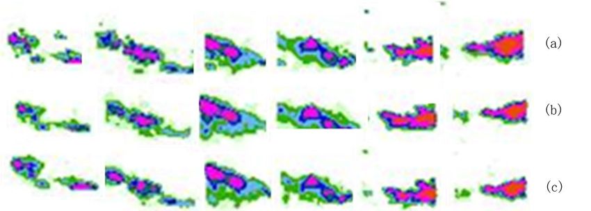
460                                                   CMC, vol.65, no.1, pp.459-479, 2020

relationship between radar echo and precipitation to do QPE [Li, Chen, Wang et al.
(2020)]. With the advent of the intelligent era, many academic scholars proposed
different types of optimization models to reduce the error in radar QPE [Lea, Loris,
Marco et al. (2018); Tao, Hsu, Ihler et al. (2018); Song, Chen, Chen et al. (2019)]. Kusiak
et al. [Kusiak, Wei, Verma et al. (2013)] verified the effectiveness of multi-layer
perceptron, random forest, SVM, classification regression tree and K-nearest neighbor
algorithm on QPE, as well as emphasizing the importance of using machine learning for
radar data driven problems. Fu et al. [Fu, Xiao, Tan et al. (2015)] improved the function
of a radial basis in the neural network model. Compared to the Z-R relationship better
accuracy and stability are acquired but only in limited experimental regions. Chen et al.
[Chen, Chen, Zhao et al. (2019)] utilized the gradient boost decision tree (GBDT) to
study meteorological radar data in South China. Its results are better than the fixed Z-R
relationship and the dynamic Z-R relationship, but the issue of inaccurate estimation is
not addressed yet. Zhang et al. [Zhang, Yang and Zhang (2019)] considered weighted
random forest as well as vertical profile of reflectivity (VPR), and analyzed radar
quantitative estimation on rainfall procedure. This work suggested that obtaining
precipitation more accurate than traditional Z-R relationship and random forest methods
is possible. The previous research is mainly based on traditional machine learning, that
suffers from a low effect on the high spatiotemporal resolution of radar.
In recent years, the spatiotemporal networks have been gaining an increasing amount of
attention from QPE researchers [Yu, Liu, Wang et al. (2018); Zuo, Yu, Zi et al. (2018);
Zhang, Jin, Sun et al. (2018); Chen, Wang, Liu et al. (2019); Wang, Liu, Xu et al.
(2019)]. A video fingerprint recognition model based on spatiotemporal deep neural
network combined with self-encoding and LSTM (Long Short-Term memory) network is
described in Wang et al. [Wang and Li (2018)]. Later, Zhang et al. [Zhang, Bai, Sha et al.
(2019)] proposed a mobile network traffic model based on spatiotemporal features, where
three-dimensional convolutional network and time convolutional network are employed
to extract the spatial characteristics of mobile network traffic, and achieved quality
results for short-term traffic prediction. Currently in the meteorological field, there are
limited studies on the application of space-time networks to radar QPE. In 2015, Shi et al.
[Shi, Chen, Wang et al. (2015)] took advantages of both the convolutional layer and the
recursive layer to present Convolutional Long Short-Term Memory (ConvLSTM) for
short-term rainfall forecasting, which partially remedied the shortcomings of the optical
flow methods by better handling image space and dynamics information. Based on the
LSTM network model, Wang et al. [Wang, Long, Wang et al. (2017)] developed radar an
echo nowcasting technology by adapting a number of existing works such as
spatiotemporal memory unit, hierarchical normalization, deconvolution network, data
augmentation. Their results show that the model extrapolates the precipitation is better
than other benchmark algorithms.
By studying the spatiotemporal characteristics of radar data and the rapid change of
rainfall data, we quantitatively estimated the precipitation of rainfall scanned by the radar
for the current 60 minutes. We analyzed the historical radar echo data of Hunan
Meteorological Observatory and propose a radar quantitative precipitation estimation
algorithm, which is referred to ST-QPE (Spatiotemporal QPE), we also designed a
convolutional time-series model QPE-Net8 and a multi-scale feature fusion time-series
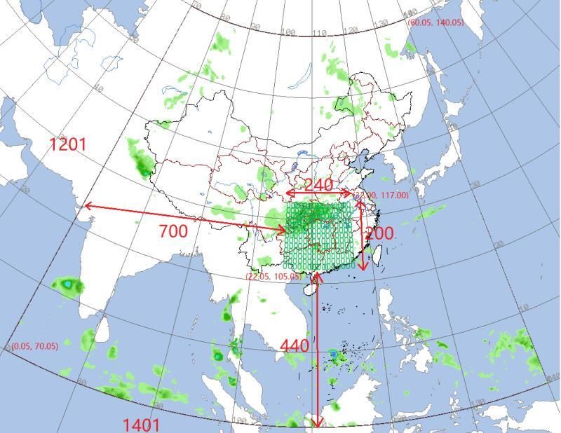
An Approach for Radar Quantitative Precipitation Estimation                                461

model QPE-Net22. We conducted a set of contrast reversal experiments with radar echo
data and rainfall data collected by the Hunan Meteorological Observatory, and applied
the statistical and meteorological tests on the ST-QPE. The experimental results showed
that our method better reflected the rainfall information corresponding to the current
radar echo than existing work.

2 Related work
QPE is mainly based on estimated precipitation from weather radar, which works as
follows: the meteorological radar emits electromagnetic waves that will get scattered due
to intersections with raindrops and snowflakes, then the radar echoes are received by
radar antenna and displayed on screens to allow meteorologists to learn the intensity,
distribution, movement and evolution of precipitation in the atmosphere according to
echo images and thus further to understand the structure and characteristics of the
weather system.

2.1 The relationship of radar echo and rainfall intensity
The Z-R relationship reflects the correlation between the radar echo and the rain-fall
intensity. Mathematically, the relationship between the radar reflectivity factor Z (unit:
mm6/m3) and the rainfall intensity R (unit: mm/h) is:
Z = aR b                                                                                (1)
where a and b are empirical constants (a≈200, b [1.5 and 2]), determined by various
factors such as time, location and type and nature of precipitation. The Z-R relationship is
the main basis for radar measurement of precipitation, and its measurement accuracy
depends on the determination of a and b parameters.

2.2 The analysis of radar and rainfall data
The weather radar collects a radar echo data Z map every 6 minutes, that is to say 240 sheets
or time series per day. Each time point contains 12 layers of radar echo data of m×n latitude
and longitude grid points (0.01°, grid point size is 1 km×1 km). Among the 12 layers, layers
1 to 10 are at height of 0.5 km, 1.0 km, 1.5 km, 2.0 km, ..., 5.0 km, the 11th layer is the echo
top height, and the 12th layer is the vertical integrated liquid water content.
The rainfall data collects a rainfall intensity R every hour. The rainfall coverage is 5
km×5 km latitude and longitude grid (the lattice distance is 0.05°), as shown in Fig. 1,
representing the radar data of 5×5 latitude and longitude grid points.
In general, radar data has time series and spatial characteristics; rainfall data is unstable
and strong in spatiotemporal characteristics, due to the rapid change of rainfall process.
462 CMC, vol.65, no.1, pp.459-479, 2020
Figure 1: Rainfall coverage map
2.3 The description of QPE
According to Eq. (1), the essence of the QPE is the problem of determining parameters a,
b based on radar data and rainfall data . However, because the model described by
Eq. (1) is too simple, it cannot reflect the spatiotemporal characteristics of well,
which makes it difficult to greatly improve the estimation accuracy. This paper attempts
to solve this problem by using the deep learning model of spatiotemporal networks.
The precipitation intensity R of a certain location (latitude and longitude) is related to the
radar echo factor at the location and its neighboring spatial points (latitude, longitude and
altitude). In other words, Z is a 3-dimensional matrix data, and the precipitation intensity
Rt at a certain time t. It can be fitted by the following network functions:
h
=Rt f= ( Z t ) f ( f ( h-1) ( Z t )),=
f (Zt ) w * Zt + b (2)
where f is the convolution function, w is the convolution kernel parameter, b is the offset
parameter, and h is the convolution depth.
Now the temporal characteristics of the radar echo data and the rainfall data can be taken
into account. According to the radar spatial data Z1, Z, …, Zt at the periodic moments of 1,
2, …,T, a more accurate precipitation intensity Rt at time t is expressed as:
Rt g ( g ( R1 , R2 , L , Rt -1 ; q ), Rt ; q ),=
= t 1, 2, …, T (3)
Therefore, the problem is to find an optimized spatiotemporal network model parameter
that makes the hit ratio of the sample data D ={ < Zt ,Rt >| t =1, 2, ,T } as large as possible.
T
θ = arg max ∑ log p(| Rt − F( Z1 ,Z 2 , ,Z t ;θ )|< ε ) (4)
θ
t =1
where F is a spatiotemporal network containing f and g, and θ is the network parameter.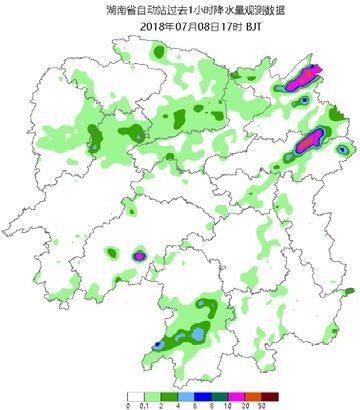
An Approach for Radar Quantitative Precipitation Estimation 463
3 Design of spatiotemporal network
For the purpose of investigating the characteristics of spatiotemporal network model in
the QPE problem, we propose a deep learning algorithm, which is able to construct a
network model not only for the QPE problem but also for more general spatiotemporal
sequence problems. Additionally, we introduce the training phase of algorithm and the
back-propagation process to evaluate model accuracy. Contributions of this paper relate
primarily to this section.
3.1 The strategy of spatiotemporal network
Based on the spatiotemporal characteristics of QPE problem, this paper designs a
spatiotemporal deep neural network algorithm model ST-QPE, which extracts the spatial
and time characteristics of the radar image respectively to finally find the rainfall amount.
The model is divided into two parts, a spatial feature layer and a temporal feature layer.
For the layer feature of space, C is the convolution operation, σ is the sigmoid activation
function, wi and bi are the convolution kernel weights and offset parameters, then a
formula is defined as Eq. (5).
Z i=0
Yi+1= (5)
σ(wi*Yi +bi ) otherwise
where i denotes the number of convolution layers, and Yi denotes the input of the i-th
layer convolution. i=0 indicates that the input of the first-layer convolution is Z. When
i>0, the output of the i-th layer is used as the input into its next layer, and the operation of
convolution activation is performed in sequence.
For the layer feature of time, It can be known from Eq. (5) that the feature value Yi +1 from
the i-th layer in the spatial feature layer is assumed to have a j-layer time series structure,
and for each time, by having the state value of the previous time set to ht −1 , the operation
of the j-th layer timing structure, when j=1:
r1t =σ(wr,1 × [h1t-1 ,Yi+1
t
])
z1t =σ(wz,1 × [h1t-1 ,yi+1
t
])
h1t tanh( wh ,1 ⋅ [ rt ∗ h1t −1 , yi+1
= t
]) (6)
h1t = ( 1 − z1t ) ∗ h1t −1 + z1t ∗ h1t
=y1t σ( wo ,1 ⋅ h1t )
When j is otherwise, the j-th layer timing structure is: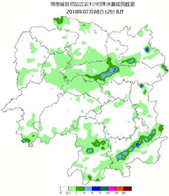
464 CMC, vol.65, no.1, pp.459-479, 2020
rjt =σ(wr,j × [ht-1 t
j ,h j −1 ])
z tj =σ(wz,j × [ht-1 t
j ,h j −1 ])
h tj tanh( wh , j ⋅ [ rjt ∗ htj−1 ,htj −1 ])
= (7)
htj = ( 1 − z tj ) ∗ htj−1 + z1t ∗ h tj
=y tj σ( wo , j ⋅ htj )
When t=1, the initial state value htj 0 of all-time feature layers is 0. In other cases, the
timing features are extracted according to Eq. (7). The overall structure of ST-QPE is
shown in Fig. 2.
R’
feature
ht-2 ConvGRUC ht-1 ConvGRUC ht ConvGRUC
layer
time
ConvGRU
ell ell ell
Spatial feature layer
Figure 2: ST-QPE structure
In this paper, two different structures, QPE-Net8 and QPE-Net22, are designed for the
connection characteristics of space and time. The difference is that when the time feature
extraction layer is carried out, two kinds of operation modes are performed on the spatial
features. QPE-Net8’s spatial feature operation is a reference structure that uses pure
convolution and pooling operations to take the extracted feature values as input into the
temporal feature layer and then perform operations involving three timings. Unlike QPE-
Net8, QPE-Net22 network uses four sub-sampling operations in the spatial feature
extraction layer to accomplish multi-scale feature recognition of images. In each layer of
timing operation sampling results of the spatial feature layer are utilized by fusing the
multi-scale features, and thoroughly connecting the spatial feature layer and the temporal
feature layer through the entire network model.
3.2 QPE-Net8
In QPE-Net8 where an 8-layer network structure is employed, convolution and pooling
operations are used to perform feature extraction to ensure a sufficient number of
convolutions to extract features, then operations are performed by ConvGRU [Shi, Gao,
Lausen et al. (2017)]. QPE-Net8 is implemented alternately by three convolutional layers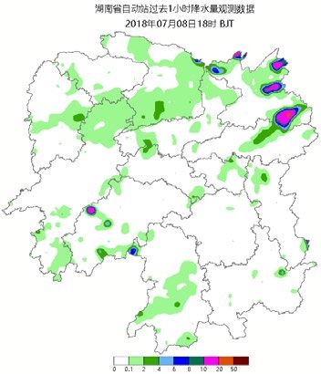
An Approach for Radar Quantitative Precipitation Estimation 465
and two maximum pooling layers for extracting radar space features, and three layers of
ConvGRU cell are used to learn radar timing features. Now the input of the timing layer
is the result of the last layer of spatial features, at any given time step:
= t
Ylast +1 ( (
σ C wi * Ylast t + bi )) (8)
For the first cell of the timing layer, the operation of the first-level timing structure
becomes:
= (
r1t σ wr ,1 ⋅ h1t −1 , Ylast
t
+1 )
=z1t σ (w t −1 t
z ,1 ⋅ h1 , Ylast +1
)
(9)
=
t
(
h1 tanh wh ,1 ⋅ r1t * h1t −1 , Ylast
t
+1 )
The timing structure of the second and third layers is identical to Eq. (7).
The structure of QPE-Net8 is shown in Fig. 3. By taking the first six layers of the radar
echo data subjected to data preprocessing as channels, inputting the radar data of 10
consecutive moments intermediate eigenvalues are obtained by applying convolution
operation to the feature layer. Eigenvalues are then input into each ConvGRU cell unit
depending on the timing. Finally, the rainfall data corresponding to the hour is generated.
The QPE-Net8 parameter configuration table is shown in Tab. 1.
Table 1: QPE-Net8 Network parameter
Input size Kernel size Output size z
224×224×6 3×3 224×224×64
224×224×64 3×3 112×112×128
112×112×128 3×3 56×56×256
Figure 3: QPE-Net8 network structure466 CMC, vol.65, no.1, pp.459-479, 2020
A typical calculation flow of the QPE-Net8 network model is presented in Algorithm 1.
Algorithm1 QPE-Net8
Input: Training data Di =,i=1,2, ,k
Output: The rainfall Y
1: for t=1, 2, …, T:
2: for i=1, 2, …, n:
3: Ct=Convi(Zt);
4: if i≠n then:
5: Ct=Maxpoolingi(C);
6: end for
7: Dt=Ct;
8: for j=1, 2, …, m:
9: Gt, ht=GRUcellj(Dt , ht-1);
10: Gt=ReLUj (Gt);
11: end for
12: end for
13: Y=ReLU(W*Gt+b);
14: return Y
3.3 QPE-Net22
Similarly, QPE-Net22 employs a 22-layer network structure. As opposed to the QPE-Net8
network, QPE-Net22 first implements multi-scale feature recognition of image features in
space, and each layer of time series operations uses the sampling results of the spatial
feature layer. Multi-scale feature fusion, the connection of the spatial feature layer and the
temporal feature layer runs through the entire network model; at the same time,
downsampling is used to reduce redundant information to form a tighter expression, making
the output feature map more accurate. The overall structure of the network is divided into
two parts: feature extraction and sampling layer. Prior to each upsampling, ConvGRU is
integrated to perform timing operations. There are four downsampling operations in the
feature extraction layer, and the output of each sampling is set to Yi +1 . Then:
z i =1
Yi +1 = (10)
σ ( C( wi * Yi + bi )) i =2,3,4
The timing layer has two layers of results. Unlike QPE-Net8, the timing result of each layer
uses the sampling result Yi +1 of the corresponding layer from bottom to top. the timing
structures of the first layer and the second layer are easily derived using Eqs. (6) and (7).An Approach for Radar Quantitative Precipitation Estimation 467
(The first layer)
= (
r1t σ wr ,1 ⋅ h1t −1 , Y5t+1 )
=z1t σ (w z ,1 ⋅ h1t −1 , y5t +1 ) (11)
=
t
(
h1 tanh wh ,1 ⋅ r1t * h1t −1 , y5t +1 )
(The second layer)
(
σ wr ,2 ⋅ h2t −1 , Y4t+1 + h1t
r2t = )
z2 t σ (w
= z ,2 ⋅ h2t −1 , y4t +1 + h1t ) (12)
t
h2 = (
tanh wh ,2 ⋅ r2t * h2t −1 , y4t +1 + h1t )
The structure of QPE-Net22 is shown in Fig. 4. Taking the first six layers from the
preprocessed radar echo data as the channel, by inputting the radar data of 10 continuous
time, each time passing through two convolutional layers, and then learning the multi-
level features through the downsampling (the largest pooling layer). Each time the
downsampling size is changed to half of the original. When upsampling, the ConvGRU
unit is used for timing calculation, and then the same number of channels corresponding
to the feature extraction part are fused, and finally the rain data corresponding to the hour
is generated. QPE-Net22 is a network parameter configuration table as shown in Tab. 2.
Table 2: QPE-Net22 Network parameter
Input size Kernel type Kernel size Output size
224×224×6 Conv2d 3×3 224×224×64
224×224×64 Downsampling conv2d 3×3 112×112×128
112×112×128 DownSampling conv2d 3×3 56×56×256
56×56×256 DownSampling conv2d 3×3 28×28×1
28×28×1 DownSampling conv2d 3×3 14×14×1
14×14×1 Upsampling deconv2d 3×3 28×28×1
28×28×1 Upsampling deconv2d 3×3 56×56×1468 CMC, vol.65, no.1, pp.459-479, 2020
Figure 4: QPE-Net22 network structure
A typical calculation flow of the QPE-Net22 network model is as follows:
Algorithm2 QPE-Net22
Input: Training data Di =,i=1,2, ,k
Output: The rainfall Y
1: for t=1, 2, …, T:
2: for i=1, 2, …, n:
3: Ci=DownConvsi (Zt);
4: end for
5: Dt=Cn;
6: for i=1, 2, …, n:
7: Dt=UpConvsj (Cn-j-1,Dt);
8: Gt, ht =GRUcellj (Dt, ht-1);
9: Gt=ReLUj (Gt);
10: end for
11: end for
12: Y=ReLU (W*Gt+b);
13: return Y
3.4 Training algorithm
The ST-QPE algorithm’s radar quantitative estimation of precipitation training process on
these two structures mentioned above is listed:An Approach for Radar Quantitative Precipitation Estimation 469
Algorithm3 ST-QPE
Input: Training data < Di ,Rl > ,Di =
< Z1 ,Z 2 , ,ZT > ,i =
1, 2 , ,k
Output: The model parameter θ =
< W ,b >
1: f ← QPENet 8 or QPENet22 ;
2: Initial θ ;
3: Do while itertime ≤ epoch and ∆ > ε :
4: L( Rt ,Di ,θ ) ← Rt − f ( Di ,θ ) ;
5: ∆= Ri − f ( Di ,θ ) ;
6: θ ← θ − η ⋅ ∇L( Rt ,Di ,θ ) ;
7: EndDo
8: Output θ
After obtaining training samples, the algorithm selects an appropriate number of batches
from the training set, use the back-propagation algorithm to find the optimal parameters,
input the training set into the ST-QPE algorithm, and iterate through the epoch to the
model convergence. ST-QPE algorithm training is actually a process of seeking the
optimal parameters. The loss function is used as the training target during model training.
this paper uses Mean Square Error (MSE) as our loss function to evaluate accuracy of
model training. The calculation formula is as Eq. (13):
1 n
=L ∑ ( y − y ' )2
n i =1
(13)
where n is the total number of experimental samples, y is the actual rainfall value, and y ′
is the result value reversed by the model.
3.5 Back propagation and parameter update
Similar to Shin et al. [Shin, Ahn, Lee et al. (2019)], we adopt Rectify Linear Unit (ReLU)
as the activation function, which helps to solve the convergence of deep networks, also to
improve the model expression ability. Because of the piecewise linear characteristics of
the ReLU function, the network does not easily lose information during forward and
backward propagation. The expression of the ReLU function is as Eq. (14):
0,x ≤ 0
f(x)= (14)
x, x>0
For the ST-QPE algorithm, the loss function is defined as L( θ ) , and the gradient of the
parameter θ is obtained by the loss function. To facilitate the derivative operation, the
calculation formula of the loss function has been improved. The back-propagation
process is as Eqs. (15) to (17):470 CMC, vol.65, no.1, pp.459-479, 2020
1 n
L( θ )
= ∑ ( y − y′( θ ))2
2n i =1
(15)
∂L 1 n ∂y ′
= ∑
∂θ n i =1
( y − y ′( θ ))
∂θ
(16)
∂L
∇θ L( θ ) = (17)
∂θ
After obtaining the gradient of each layer, we use the stochastic gradient descent
algorithm to update the parameters of each layer so that the objective function converges.
the magnitude of the parameter change is adjusted by referring to the learning rate η
according to the gradient, as shown in the Eq. (18):
θ= θ − η ⋅∇θ L( θ ) (18)
An inappropriate value of η can introduce issues. The network may converge too slow if
the value is too small, or may never converge if the value is too large. Empirically, the
learning rate of this paper is best when it is set to 0.001.
4 Experimental results and analysis
The method is implemented using python with a deep learning framework pytorch on
pycharm. To demonstrate the method, we also take the advantage of GPU computing
architecture to gain higher performance by using CUDA 9.0 and CUDNN. We conducted
experiments for analysis of QPE-Net8 and QPE-Net22 on a computer with an NVIDIA
GTX 1080Ti card.
4.1 Dataset
Meteorological observation data is a collection of various raw data observed by
conventional meteorological instruments and professional meteorological equipment.
The meteorological element sequences accumulated from continuous observations at
fixed points, cannot directly represent the characteristics of regional climate change in
climate analysis and numerical simulation, due to limitations such as uneven station
spatial distribution, uneven sequence lengths instability of observation equipment in
performance. Therefore, such data encounters many restrictions in practical applications.
Motivated by these limitations, this paper systematically integrates and perform quality
control on the experimental samples. We choose radar data and rainfall data from
February to October 2018 as experimental data. The string-matching algorithm is used to
select the effective samples of the radar data. 7450 consecutive valid samples are selected
among 11162 samples; thus 745 rainfall sets of data. In order to speedup reading, the
original radar echo data and the rainfall data that covers the whole province are cropped
with a smaller size of 45×45 (550 to 595, 840 to 885). The size of original coverage is
224×224 (550 to 774, 700 to 924). The radar echo data values are normalized, level by
level to between 0 and 1 using Eq. (19):An Approach for Radar Quantitative Precipitation Estimation 471
xi − xmini
=xi' (0 ≤ i472 CMC, vol.65, no.1, pp.459-479, 2020
Figs. 5-8 shows the changes of the loss values of QPE-Net8 and QPE-Net22 after 300
iterations. It can be seen from the figure that as the number of iterations increases, the
loss values of the two structures gradually decrease and tend to be stable.
Now we can draw the inversion rainfall map based on the optimal model. Fig. 9 is a
comparison of rainfall images retrieved from radar echo maps between CMPA, QPE-
Net8 and QPE-Net22. Darker colors indicate greater rainfall intensity. By having the loss
maps of both two structures, the QPE-Net8 and QPE-Net22 network structures are able to
learn the radar data characteristics to get inversed rainfall maps that are more similar to
and the real rainfall maps.
Figure 9: The rainfall images retrieved from radar echo maps. (a) the CMPA hourly
fusion live rainfall map (the label), (b) the rainfall map retrieved by QPE-Net8, (c) the
rainfall map retrieved by QPE-Net22
Then, we use the MICAPS, a comprehensive analysis and processing system for weather
information, to visualize the map on July 6, 2018 at 05:00, where the size is 45×45 with
the grid interval of 0.05, longitude from 112° E to 114.2° E and latitude from 27.5° N to
29.7° N. The result is then converted into Micaps fourth type data format. The data is
arranged in the wise of first weft and backward meridian. Next, data from label, QPE-
Net8, and QPE-Net22 are imported into the Micaps system with the region set to Hunan.
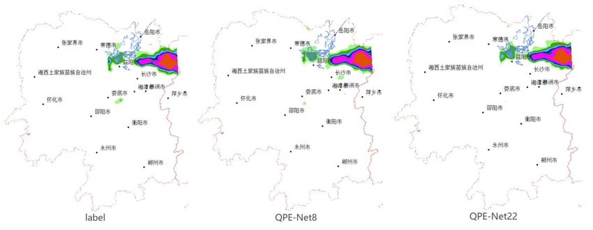
The results are shown in Fig. 10 and the enlarged area is shown in Fig. 11.
Figure 10: The result comparison in MICAPSAn Approach for Radar Quantitative Precipitation Estimation 473
Figure 11: The enlarged area map
As can be seen from Figs. 11 and 12, a clearer and more intuitive understanding of the
results can be developed, by visualizing CMPA fusion hourly live, and results of QPE-
Net8 and QPE-Net22 inversion. Compared with the CMPA actual situation, results show
that the QPE-Net8 and QPE-Net22 models have better responses in several heavy
precipitation centers, therefore better reflect the heavy precipitation area where the
overall deviation of precipitation is relatively small. Fig. 11 shows the QPE-Net8
underestimates the heavy rainfall center, while the QPE-Net22 model based on multi-
scale fusion is stronger than the CMPA live and QPE-Net Net8 model has better stability.
4.3 Test of results
In order to describe the error and accuracy characteristics of radar retrieval rainfall effect,
this paper uses the Mean-Square Error (MSE), Mean Error (ME) and Relative Error (RE)
to statistically evaluate these two models by Eqs. (21)-(23). RMSE is used to measure the
similarity between predicted results and label values, which is commonly used in
regression problems in the field of machine learning. Use RMSE to evaluate the
dispersion of QPE-Net8, QPE-Net22 and CMPA live rainfall. If the RMSE is smaller, it
means that the distribution is more concentrated. The average error is used to estimate the
overall data difference. The closer the ME is to 0, the smaller the overall data difference;
The relative error is used to estimate the reliability of the data. The smaller the RE, the
higher the reliability of the data.
1 n
RMSE
= ∑
n i =1
( y − y ' )2 (21)
1 n
ME
= ∑ ( y − y' )
n i =1
(22)
1 n
∑ y − y'
n i =1
=RE × 100% (23)
1 n '
∑y
n i =1474 CMC, vol.65, no.1, pp.459-479, 2020
where n represents the total number of samples, y is the sample label, and y is the
'
value inversed by the model.
In order to ensure the evaluation objectivity of, this paper divides rainfall into light rain
(less than or equal to 2.5 mm), moderate rain (2.6~8.0 mm), heavy rain (8.1~15 mm), and
torrential rain (more than or equal to 16 mm) according to the one-hour rainfall level.),
the rainfall inversion of the two models is analyzed for each group.QPE-Net8 and QPE-
Net22 models and CMPA live rainfall scatter plots are given in Fig. 12. The closer the
points lie on a scatter plot with respect to the straight line, the better the radar rainfall
inversion quality is. Points above and under the line indicate overestimation and
underestimation respectively. As shown in Fig. 12, in the case of QPE-Net8
underestimation become more obvious as the amount of rainfall increases. the correlation
coefficient between QPE-Net22 and CMPA live rainfall is slightly higher than that of
QPE-Net8, indicating that QPENet22 has a better correlation with CMPA live
distribution, as a more concentrated distribution can be observed, which effectively
improves the accuracy of rainfall estimation. Therefore, the QPE-Net22 network gives
inversion closer to the CMPA hourly live than QPE-Net8 does.
Figure 12: The scatter plot of CMPA live, QPE-Net8 estimated rainfall and QPE-Net22
estimated rainfall
Then, based on the rainfall level, we give the error analysis of QPE-8 and QPE-Net22
models, as shown in Tab. 4.
Table 4: The analysis of radar inversion rainfall error for different rainfall levels
Model 16 mm
RMSE 2.4608 7.8636 14.641 19.789
QPE-Net8 ME 0.1976 -0.0668 0.0106 0. 1093
RE 0.5129 0.3088 0.0339 0.0942
RMSE 2.4873 7.8636 14.556 17.609
QPE-Net22 ME 0.0393 -0.0103 0.0314 0. 0297
RE 0.1732 0.0378 0.0942 0.0275An Approach for Radar Quantitative Precipitation Estimation 475
According to Tab. 4, QPE-Net8 and QPE-Net22 overestimate the rainfall more often for
light rain, heavy rain and torrential rain, but highly underestimate moderate rain. The
QPE-Net22 model has an average error of 0.0297 mm and a relative error of 0.0275, In
this order of magnitude, rainfall is better than the QPE-Net8 model, and the average error
of QPE-Net8 overestimation of heavy rain is 0.0106 mm and the relative error is 0.0339,
which is better than the QPE-Net22 model. Overall, QPE-Net22 has average and relative
retrieval errors on cases of light rain, moderate rain, and heavy rain lower than QPE-
Net8. For moderate rain, heavy rain, and torrential rain, the mean square error generated
by QPE-Net22 is also smaller than QPE-Net8, which indicates that QPE-Net22 has a
higher degree of fit for heavy rainfall and torrential rainfall.
Finally, we use the objective weather testing methods for ConvGRU, QPE-Net8 and
QPE-Net22, including the Probability of Detection (POD), the False Alarm Ratio (FAR),
and the Critical Success Index (CSI) [Lu, Ren, Sun et al. (2018)]. The calculation
formulas are shown in Eqs. (24)-(26).
TP
POD = (24)
TP + FN
FP
FAR = (25)
TP + FP
TP
CSI = (26)
TP + FN + FP
where TP, FN and FP respectively represent the number of points in cases of the success,
false and missing reports on the inverse rainfall map.
According to the information of radar and the rainfall label, the corresponding hourly
rainfall maps are inverted, and the two network structures of QPE-Net8 and QPE-Net22
are tested and evaluated. The inversed results are tested by calculating the rainfall in each
grid cell. Evaluation and comparison analysis are performed against with the existing
ConvGRU network model. The final evaluation results are shown in Tab. 5.
Table 5: Comparison of inspection results
Model POD FAR CSI
ConvGRU 0.6342 0.2351 0.5472
QPE-Net8 0.5991 0.0246 0.5902
QPE-Net22 0.5255 0.0103 0.5226
It can be seen from Tab. 5 that POD and CSI values of QPE-Net8 and QPE-Net22 are
less than those of ConvGRU, which indicates that the rainfall results reversed by the ST-
QPE model are more stable, especially for the case of missing reports, which is referred
to FAR Evaluation. QPE-Net8 and QPE-Net22 results are significantly better than
ConvGRU. In summary, QPE-Net22 provides results that are closer to the ground truth
rainfall value than the other two methods.
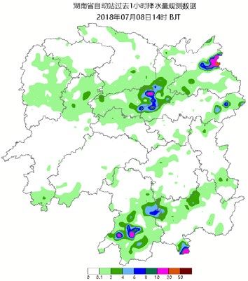
Fig. 13 shows a schematic diagram of the rainfall changes at 12, 14, 17 and 18 o’clock on
8th July, 2018. A rainfall zone including Yiyang and Yueyang is involved. As time476 CMC, vol.65, no.1, pp.459-479, 2020
advances, the rainfall has changed significantly. At 14:00, 17:00, and 18:00, rainfall of
more than 10mm appeared, followed by two zones with heavy rainfall greater than 16mm
at 17:00 and 18:00. The hourly precipitation evolution chart shows that the center of
precipitation gradually moves westward and northward over time. Fig. 13 contains the
live rainfall map obtained from the automatic station, the CMPA live area zoomed-in
map, the QPE-Net8 reversed area zoomed-in map, and the QPE-Net22 reversed area
zoomed-in map. Compared with the real station rainfall, the CMPA live rainfall, QPE-
Net8 inversion rainfall and QPE-Net22 inversion rainfall precipitation distribution and
landing area are more consistent, which further verifies the reliability of the method
presented in this paper.
Figure 13(a): The rainfall data of Hunan Province Automatic Observation Station in hour
Figure 13(b): CMPA Live Rainfall
Figure 13(c): The rainfall inversion by QPE-Net8 model
Figure 13(d): The rainfall inversion by QPE-Net22 model
Figure 13: Diagram of rainfall process from 12:00 pm to 18:00 pm on July 8, 2018An Approach for Radar Quantitative Precipitation Estimation 477 In terms of the effect of the inversion of rainfall given in Figs. 13(c) and 13(d), the overall performance of both models is relatively stable, especially for moderate rain, heavy rain and storm in the northeast border area of Hunan. In contrast to the automatic station live and CMPA live rainfall, the area and intensity of different grades of rainfall have better improvements. The spatial and temporal characteristics of QPE-Net8 are generally poorer, resulting in a narrow precipitation range and large instability. Another concern is that QPE-Net22 can generate results closer to the CMPA reality, and it is able to better grasp the northward movement of rainfall zones. The area and range of the rainstorm are more consistent with the automatic station reality and the CMPA reality. The model inversion effect better. 5 Conclusion and future work In this paper, an algorithm of radar echo precipitation based on spatiotemporal network is proposed to meet the high resolution in radar quantitative precipitation estimation which is difficult to achieve by traditional methods. The convolutional neural network was used to extract the spatial and temporal characteristics of the radar echo map, two different network structures have been designed for inversion experiments, and the ST-QPE algorithm inversion was analyzed using statistical tests and weather methods. The simulation results include the indicators and correlation coefficient diagrams of the two models for different rainfall distributions. The experimental results show that the ST-QPE algorithm can better reflect the rainfall information corresponding to the current hourly radar echo and improve the accuracy of the quantitative rainfall estimation. Therefore, useful practical guidance for small areas without radar stations and early warnings of extreme weather can be provided more efficiently. There are several avenues for future works. We would like to design a data set that includes multiple meteorological elements (such as temperature and humidity), and construct a network model that integrates attention mechanisms, optimizes network parameters. Also, improvements to the spatial and temporal characteristics can likely to be considered. Acknowledgement: We thank anonymous reviewers for their feedback which helped in the improvement and presentation of this article. We also acknowledge Professor Feibo Jiang (Hunan Normal University, China) for his feedback on an earlier version of the manuscript. Finally, we acknowledge the data support provided by the Hunan Meteorological Observatory. Funding Statement: This work is supported by the Key Research and Development Program of Hunan Province (No. 2019SK2161) and the Key Research and Development Program of Hunan Province (No. 2016SK2017). Conflicts of Interest: The authors declare that they have no conflicts of interest to report regarding the present study.
478                                                  CMC, vol.65, no.1, pp.459-479, 2020

References
Chen, X. L.; Chen, Y. Z.; Zhao, C. Y.; Zhang, K. (2019): Application of gradient boost
decision tree in radar quantitative precipitation estimation. Advances in Meteorological
Science and Technology, vol. 9, no. 3, pp. 132-137.
Chen, Y. T.; Wang, J.; Liu, S. J.; Chen, X.; Xiong, J. et al. (2019): Multiscale fast
correlation filtering tracking algorithm based on a feature fusion model. Concurrency and
Computation: Practice and Experience, pp. e5533.
Fu, D. S.; Xiao, C.; Tan, C.; Yu, B. L.; Xu, B. (2015): Application of RBF neural
network in radar quantitative precipitation estimation. Journal of the Meteorological
Sciences, vol. 35, no. 2, pp. 199-203.
Kusiak, A.; Wei, X.; Verma, A.; Roz, E. (2013): Modeling and prediction of rainfall
using radar reflectivity data: a data-mining approach. IEEE Transactions on Geoscience
and Remote Sensing, vol. 51, no. 4, pp. 2337-2342.
Lea, B.; Loris, F.; Marco, G.; Ulrich, H. (2018): Satellite-based rainfall retrieval: from
generalized linear models to artificial neural networks. Remote Sensing, vol. 10, no. 6, pp.
1-24.
Li, X.; Chen, Y. B.; Wang, H. Y.; Zhang, Y. Y. (2020): Assessment of GPM IMERG
and radar quantitative precipitation estimation (QPE) products using dense rain gauge
observations in the Guangdong-Hong Kong-Macao greater bay area, China. Atmospheric
Research, vol. 236, pp. 1-67.
Lu, Z. Y.; Ren, Y. M.; Sun, X. L.; Jia, H. Z. (2018): Recognition of short-time heavy
rainfall based on deep learning. Journal of Tianjin University (Science and Technology),
vol. 51, no. 2, pp. 111-119.
Shi, X. J.; Chen, Z. R.; Wang, H.; Yeung, D. Y.; Wong, W. K. et al. (2015):
Convolutional LSTM network: a machine learning approach for precipitation nowcasting.
Advances in Neural Information Processing Systems, pp. 802-810.
Shi, X. J.; Gao, Z. H.; Lausen, L.; Wang, H.; Yeung, D. Y. et al. (2017): Deep
learning for precipitation nowcasting: a benchmark and a new model. Advances in Neural
Information Processing Systems, pp. 5620-5630.
Shin, H. K.; Ahn, Y. H.; Lee, S. H.; Kim, H. Y. (2019): Digital vision based concrete
compressive strength evaluating model using deep convolutional neural network.
Computers, Materials & Continua, vol. 61, no. 3, pp. 911-928.
Song, L. Y.; Chen, M. X.; Chen, C. L.; Gao, F.; Chen, M. (2019): Characteristics of
summer QPE error and a climatological correction method over Beijing-Tianjin-Hebei
region. Acta Meteorologica Sinica, vol. 3, no. 3, pp. 497-515.
Tao, Y.; Hsu, K.; Ihler, A.; Gao, X. (2018): A two-stage deep neural network
framework for precipitation estimation from bispectral satellite information. Journal of
Hydrometeorology, vol. 19, no. 2, pp. 393-408.
Wang, D. D.; Li, Y. N. (2018): Video fingerprint algorithm based on spatio-temproal
deep neural network. Laser & Optoelectronics Progress, vol. 55, no. 1, pp. 1-7.
Wang, L.; Liu, J. P.; Xu, S. H.; Dong, J. J.; Yang, Y. (2018): Forest above ground
biomass estimation from remotely sensed imagery in the mount tai area using the RBF
An Approach for Radar Quantitative Precipitation Estimation                       479

ANN algorithm. Intelligent Automation and Soft Computing, vol. 24, no. 2, pp. 391-398.
Wang, Y. B.; Long, M. S.; Wang, J. M.; Gao, Z. F.; Yu, P. S. (2017): PredRNN:
recurrent neural networks for predictive learning using spatiotemporal LSTMs. Advances
in Neural Information Processing Systems, pp. 879-888.
Yu, R. G.; Liu, Z. Q.; Wang, J. R.; Zhao, M. K.; Gao, J. et al. (2018): Analysis and
application of the spatio-temporal feature in wind power prediction. Computer Systems
Science and Engineering, vol. 33, no. 4, pp. 267-274.
Zhang, C. Y.; Yang, X. B.; Zhang, W. S. (2019): Accurate precipitation nowcasting
with meteorological big data: machine learning method and application. Journal of
Agricultural Big Data, vol. 1, no. 1, pp. 78-87.
Zhang, J. M.; Jin, X. K.; Sun, J.; Wang, J.; Sangaiah, A. K. (2018): Spatial and
semantic convolutional features for robust visual object tracking. Multimedia Tools and
Applications.
Zhang, J.; Bai, G. W.; Sha, X. L.; Zhao, W. T.; Shen, H. (2019): Mobile traffic
forecasting model based on spatio-temporal features. Computer Science, vol. 46, no. 12,
pp. 108-113.
Zuo, X. Q.; Yu, H. C.; Zi, C. B.; Xu, X. K.; Wang, L. Q. et al. (2018): Meteorological
correction model of IBIS-L system in the slope deformation monitoring. Intelligent
Automation and Soft Computing, vol. 24, no. 1, pp. 47-54.
You can also read