Adaptive Blending Method of Radar-Based and Numerical Weather Prediction QPFs for Urban Flood Forecasting - MDPI
←
→
Page content transcription
If your browser does not render page correctly, please read the page content below
remote sensing
Article
Adaptive Blending Method of Radar-Based and
Numerical Weather Prediction QPFs for Urban
Flood Forecasting
Seong-Sim Yoon
 Korea Institute of Civil Engineering and Building Technology, Goyang-Si, Gyeonggi-Do 10223, Korea;
 ssyoon@kict.re.kr; Tel.: +82-31-910-0720

 Received: 30 January 2019; Accepted: 13 March 2019; Published: 16 March 2019

 Abstract: Preparing proper disaster prevention measures is important for decreasing the casualties
 and property losses resulting from floods. One of the most efficient measures in this regard is
 real-time flood forecasting using quantitative precipitation forecasts (QPFs) based on either short-term
 radar-based extrapolation or longer-term numerical weather prediction. As both methods have
 individual advantages and limitations, in this study we developed a new real-time blending technique
 to improve the accuracy of rainfall forecasts for hydrological applications. We tested the hydrological
 applicability of six QPFs used for urban flood forecasting in Seoul, South Korea: the McGill Algorithm
 for Prediction Nowcasting by Lagrangian Extrapolation (MAPLE), KOrea NOwcasting System
 (KONOS), Spatial-scale Decomposition method (SCDM), Unified Model Local Data Assimilation
 and Prediction System (UM LDAPS), and Advanced Storm-scale Analysis and Prediction System
 (ASAPS), as well as our proposed blended approach based on the assumption that the error of the
 previously predicted rainfall is similar to that of current predicted rainfall. We used the harmony
 search algorithm to optimize real-time weights that would minimize the root mean square error
 between predicted and observed rainfall for a 1 h lead time at 10 min intervals. We tested these
 models using the Storm Water Management Model (SWMM) and Grid-based Inundation Analysis
 Model (GIAM) to estimate urban flood discharge and inundation using rainfall from the QPFs as
 input. Although the blended QPF did not always have the highest correlation coefficient, its accuracy
 varied less than that of the other QPFs. In addition, its simulated water depth in pipe and spatial
 extent were most similar to observed inundated areas, demonstrating the value of this new approach
 for short-term flood forecasting.

 Keywords: floods; short-term forecasting; blended QPF; hydraulic modelling

1. Introduction
      Recent climate changes and abnormal weather phenomena have resulted in increased occurrences
of localized torrential rainfall in urban areas, such the notable flood disasters in Seoul, South Korea
in 2010 and 2011. Aspects of urban hydrological environments (such as reduced concentration time,
decreased storage rate, and increased peak discharge) have changed in relation to precipitation,
altering and accelerating the severity of flood damage in such areas. Thus, effective disaster prevention
measures are increasingly important for decreasing flood-related casualties and property losses. One
of the most efficient measures is real-time flood forecasting using quantitative precipitation forecasts
(QPFs). Because real-time flood prediction requires sufficient lead time for effective responses, it is
common to use rainfall forecasts produced from radar or numerical weather prediction models.
However, because these are constrained by uncertainties in the forecasting process (such as differing
algorithms or input data), the actual and predicted flood processes differ in time, volume, and
spatial extent.

Remote Sens. 2019, 11, 642; doi:10.3390/rs11060642                      www.mdpi.com/journal/remotesensing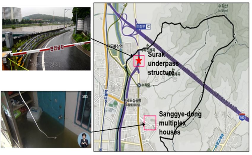
Remote Sens. 2019, 11, 642                                                                         2 of 19

      Radar-based nowcasting issues short-term forecasts (1–6 h) using extrapolation, translation, and
storm-cell tracking methods without dynamic atmospheric analysis; its accuracy, therefore, decreases
as the lead time increases because it cannot resolve the growth and decay of storms. In contrast,
numerical weather prediction (NWP) depends on synoptic observations and dynamic atmospheric
analysis to produce more reliable forecasts of convection growth and decay with longer lead times.
However, the problem of model spin-up time is a significant limitation to the application of NWP
models to the nowcasting of precipitation [1,2].
      In order to provide more accurate predictions with longer lead times, blending techniques
combining NWP models with radar-based forecasts are widely utilized. The first blended forecasts
were the Nowcasting and Initialization of Modelling Using Regional Observation Data System
(NIMROD) and the Generating Advanced Nowcasts for Deployment in Operational Land Surface
Flood Forecasting (GANDOLF) systems [3,4]. More recent nowcasting systems using this approach
include Rainstorm Analysis and Prediction Integrated Data-processing System (RAPIDS) and
Short-Term Ensemble Prediction System (STEPS) [5,6].
      The most important issue when applying the blending method is how to weight spatial
and temporal factors. Optimal predictions can be obtained by assigning weights obtained from
extrapolation forecasts for the first few hours and from NWP models afterward [3,5,7]. Lin et al. [8]
attempted to optimize a blending scheme statistically by exploring the best lead time with changing
products in an operational configuration. This approach was further addressed by Ebert and Seed [9],
who outlined the limitations of blended methods. In order to compensate for these limitations, a recent
trend toward offering probabilistic forecasts (including uncertainty of precipitation rather than simple
deterministic forecasts of location and quantity) has been explored.
      Most previous studies dealing with blending radar-based extrapolation and NWP models used a
sum of weights calculated from both fields. Such weighting functions are determined by the predictive
ability of these methods as derived from suitable quality metrics including deterministic [3,10] or
probabilistic [6] measurements based on radar reflectivity [11], rainfall rate [3], or probability of
precipitation [12]. The performance of such methods has been examined by applying linear [7] or
exponential [13] weights to the models. Additionally, a scale-dependent stochastic approach to
calculating probabilistic precipitation forecasts was applied by Bowler et al. [6].
      Blending techniques can also be divided into deterministic and adaptive techniques depending
on how weights are updated for merging [14]. The former blends a local forecast (at a point based on
observed persistence or a trend at that location) and an NWP model forecast in a weighted average,
where the weights of the two components vary with time t according to a deterministic formula.
However, this method is unnecessarily limited in use, and there has been a recent trend away from
simple deterministic forecasts of precipitation location and quantity toward offering probabilistic
forecasts that include a measure of uncertainty. As the relative reliability of local and model forecasts
vary, a method that accounts for the recently observed performance of both can be used to adapt the
weights used for blending. The adaptive method used for this purpose can itself have significant
time-dependent errors. Whether such risks outweigh the benefits of adaptation is something that must
be decided individually (i.e., by variable, location, or season, etc.).
      A number of adaptive blending schemes are more sophisticated than the deterministic blending
described above, all of which are based on forecasting the change from present conditions and adding
that change to the current observed value. In order to complement the limitations of blending
techniques using weights derived from statistical analyses, in this study we developed a real-time
adaptive blending technique that better reflects the variability of storms. We then analyzed the
hydrological applicability of each QPF approach to urban flood forecasting.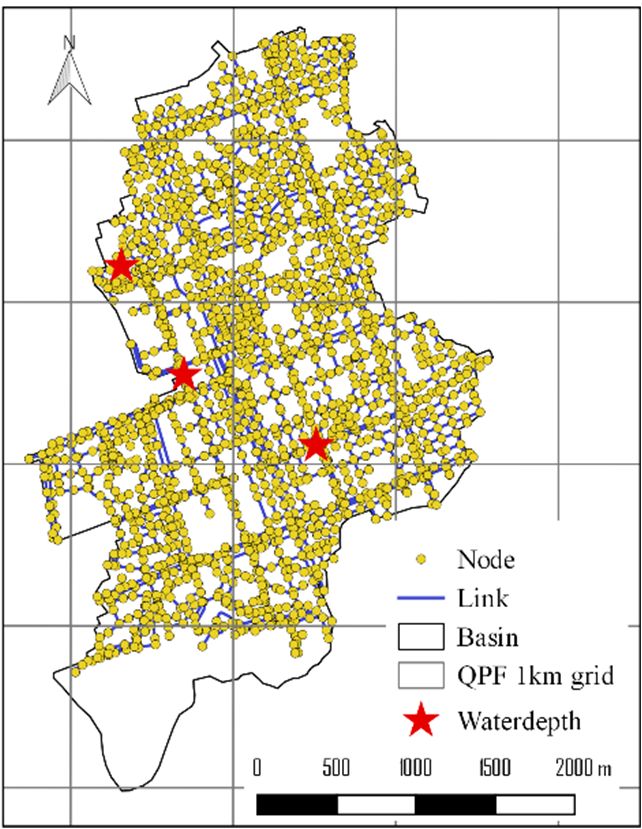
Remote Sens. 2019, 11, 642                                                                                        3 of 19
Remote Sens. 2019, 1, x FOR PEER REVIEW                                                                          3 of 18

2.
2. Materials
   Materials and
             and Methods
                 Methods

2.1.
2.1. Data
     Data and
          and Study
              Study Area
                    Area
2.1.1. Radar-Based QPFs
 2.1.1. Radar-Based QPFs
      We used three kinds of radar-based QPF data in this study, all of which were generated with 1 km
      We used three kinds of radar-based QPF data in this study, all of which were generated with 1
spatial resolution and 10 min temporal resolution. The longest prediction lead-time was 6 h.
 km spatial resolution and 10 min temporal resolution. The longest prediction lead-time was 6 h.
      The first QPF was generated by the Spatial-scale Decomposition method (SCDM) used to forecast
      The first QPF was generated by the Spatial-scale Decomposition method (SCDM) used to forecast
differential motions (such as for convective or stratiform cells) in the same precipitation system,
 differential motions (such as for convective or stratiform cells) in the same precipitation system,
following the procedures shown in Figure 1. The rainfall field was separated using image filtering,
 following the procedures shown in Figure 1. The rainfall field was separated using image filtering, the
the movement of small-scale rainfall fields (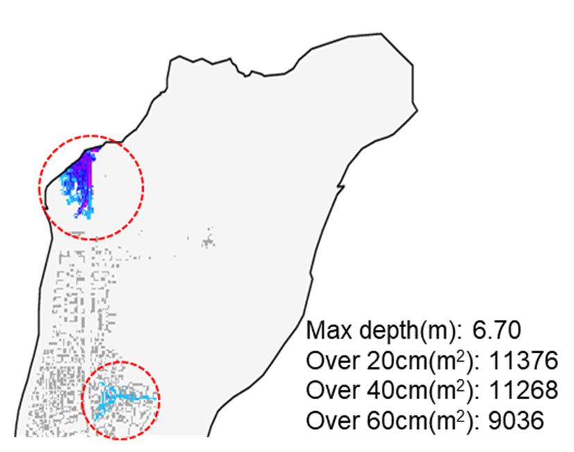
Remote Sens. 2019, 11, 642                                                                       4 of 19

every 10 min. However, it does not incorporate a dynamic precipitation process, which is a fundamental
limitation that causes lower prediction scores beyond three hours from initiation. Germann et al. [18]
discussed sources of uncertainty in MAPLE predictions associated with the growth or dissipation of
precipitation echoes as well as with changes in the echo motion field over the forecast period.
      KONOS is a new system that was developed to combine the advantages of MAPLE and
very-short-range forecasting (VSRF) to improve the predictability of very short-range forecasts. The
initial field used for the extrapolation of KONOS was a Radar-AWS Rainrate system (RAR) used to
calibrate the rain intensities (AWS stands for automatic weather stations). The echo-moving vectors
for extrapolation were then calculated by the variational echo tracking (VET) algorithm in MAPLE.
The semi-Lagrangian method in MAPLE was applied to extrapolate the initial rain intensities [19].

2.1.2. Numerical Weather Prediction Models
      We used NWP products estimated by the KMA using the Unified Model Local Data Assimilation
and Prediction (UM LDAPS) along with the Advanced Storm-scale Analysis and Prediction System
(ASAPS). KMA releases weather forecast data based on the UM 1.5 km L70, an operational short-range
local NWP suite introduced in 2012 that runs four times daily (00/06/12/18 UTC) to produce 36 h
forecasts with three hourly 3DVAR cycles, and Korea Local Analysis and Prediction System (KLAPS)
(5 km L40), a local VSRF system that analyzes weather conditions around the Korean Peninsula every
hour. Regarding the UM LDAPS data, we could not change the original settings of the KMA numerical
weather prediction model. Although the original UM LDAPS data have a 1.5 km resolution, we
interpolated these data to a 1 km resolution to maintain a homogeneous spatial resolution with the
other QPFs and for convenience when applying the blending method [20].
      KMA also employs the National Oceanic and Atmospheric Administration (NOAA)’s Local
Analysis and Prediction System (LAPS), which provides the hot-start initial condition to the ASAPS
based on the Weather Research and Forecasting (WRF) model [21]. LAPS is a meteorological data
assimilation tool that employs a suite of observations to generate a realistic, spatially distributed,
time-evolving, and three-dimensional representation of atmospheric features; this also provides the
initial condition to the forecasting system. ASAPS was developed for monitoring severe weather and
consists of a 265 × 265 km grid with a spatial resolution of 1 km centered on the Seoul metropolitan
area and performs six-hour forecasts with one-hour intervals.

2.1.3. Study Area
     Seoul is one of the most highly urbanized cities in South Korea with several residential areas and
industrial facilities located near flood plains that are at risk from damage caused by urban flooding.
Several researchers, and even the South Korean government, have worked to develop flood forecasting
systems and methodologies for urban flood disaster mitigation [22–24]. Moreover, many kinds of
QPF data are issued for the Seoul metropolitan area by the KMA, allowing us to easily evaluate the
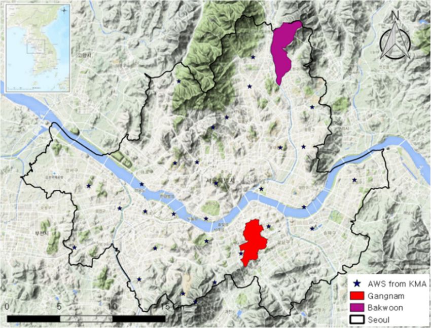
hydrological applicability and accuracy of various QPFs. We chose two specific drainage basins within
Seoul (Gangnam and Bakwoon) as shown in Figure 2. Gangnam is representative of Seoul’s downtown
area where residential and commercial areas are concentrated; this is a low-lying location with a more
complicated sewer network than surrounding areas, making this area vulnerable to flooding during
heavy rainfall. Bakwoon basin, in the northern part of Seoul near the Jung-rang River, is a residential
area that also suffers from river flooding and inundation.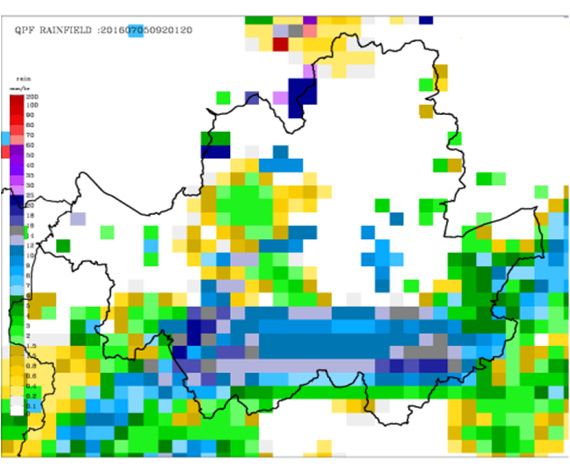
Remote Sens. 2019, 11, 642                                                                                      5 of 19
Remote Sens. 2019, 1, x FOR PEER REVIEW                                                                        5 of 18

      Figure 2.
      Figure 2. Boundary
                Boundary of
                          of the
                              theSeoul
                                  Seoulmetropolitan
                                        metropolitanarea
                                                     areafor
                                                          forwhich
                                                              whichquantitative
                                                                    quantitativeprecipitation
                                                                                  precipitation forecasts (QPFs)
                                                                                                forecasts (QPFs)
      were obtained, locations  of  Korea Meteorological Administration’  (KMA’s)    automatic  weather
      were obtained, locations of Korea Meteorological Administration’ (KMA’s) automatic weather stationsstations
      (AWS), and
      (AWS),  and boundaries
                  boundariesof  ofthe
                                   theGangnam
                                       Gangnamand
                                                andBakwoon
                                                     Bakwoon basins studied
                                                               basins       in detail.
                                                                      studied  in detail.

2.2.
2.2. Methodology
     Methodology

2.2.1.
2.2.1. Adaptive
       Adaptive Blending
                Blending Using
                         Using the
                               the Harmony
                                   Harmony Search
                                           Search Algorithm
                                                  Algorithm
      We
      We developed
           developed anan adaptive
                            adaptive blending
                                      blending method
                                                 method toto find
                                                              find the
                                                                   the optimal
                                                                        optimal weight
                                                                                 weight for
                                                                                          for real-time
                                                                                               real-time blending
                                                                                                           blending
of  the  three   QPFs   at  each  forecast  time  using   the   harmony     search   (HS)   method.
of the three QPFs at each forecast time using the harmony search (HS) method. This is a metaheuristic    This is a
metaheuristic
music-inspiredmusic-inspired
                   algorithm usedalgorithm      used range
                                    to solve a wide   to solve   a wide range
                                                            of optimization       of optimization
                                                                               problems               problems
                                                                                           in different           in
                                                                                                         fields [25–
different  fields [25–28].  When  musicians   compose   a  harmony,    they test various  possible
28]. When musicians compose a harmony, they test various possible combinations of the pitches        combinations
of the pitches
stored  in theirstored in their
                  memory,       memory,
                             which        which
                                     can be       can be considered
                                             considered                 as an optimization
                                                          as an optimization     process that process  that
                                                                                                 adjusts  theadjusts
                                                                                                              input
the  input  (pitches) to obtain  the optimal   output  (perfect  harmony).    This  approach    has
(pitches) to obtain the optimal output (perfect harmony). This approach has two essential parameters:two   essential
parameters:
the harmonythe     harmony
                memory        memory considering
                           considering  rate (HMCR)rateand(HMCR)
                                                             the pitchand  the pitch
                                                                        adjusting     adjusting
                                                                                   rate (PAR). rate (PAR).
      The HS process follows four steps (Figure 3). First, the harmony memory (HM) is initialized,
consisting of a given number of randomly generated solutions to the optimization problems. Second, a
new solution vector is improved from the HM, with each component of the solution obtained based on
the HMCR through memory considerations, pitch adjustments, and a randomization process. Third, the
HM is updated and the new solution from step two is evaluated. If it yields a better fitness than that of
the worst member in the HM, it will replace that one; otherwise it is eliminated. Fourth, steps two and
three are repeated until a preset termination criterion (e.g., the maximal number of iterations) is met.
      The proposed blending technique is based on the assumption that the error of previously predicted
rainfall is similar to current predicted rainfall. Weights are calculated every 10 min using ground
observation rainfall data that correspond to past forecast precipitation. Using Equation (1), the sum of
each weight shall be 1 + α, where α is intended to compensate for the quantitative errors of past ground
observation and forecasted rainfall. The combined weights of Equation (1) are then determined to
minimize the root mean square error (RMSE) between previous predicted rainfall and observed gauge
rainfall for the previous one-hour lead time every 10 min, as in Equations (2) and (3). The blended
QPF is estimated by Equation (4).

                             C MAPLE + CKONOS + CSCDM + CUM + C ASAPS = 1 + α,                                      (1)

                                              Fitness = min[ RMSE],                                                 (2)

      Figure 3. QPF blending process using the harmony search algorithm. HS = harmony search; HM =
      harmony memory; HMCR = harmony memory considering rate; PAR = pitch adjusting rate.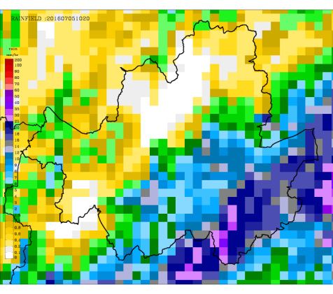
Figure 2. Boundary of the Seoul metropolitan area for which quantitative precipitation forecasts (QPFs)
         were obtained, locations of Korea Meteorological Administration’ (KMA’s) automatic weather stations
         (AWS), and boundaries of the Gangnam and Bakwoon basins studied in detail.
Remote Sens. 2019, 11, 642                                                                                         6 of 19
   2.2. Methodology
                                          v
   2.2.1. Adaptive Blending Using the u   Harmony
                                              1 N  Search Algorithm 2
                                          u
                                 RMSE = t ∑ Rtgauge − RtBLENDED , and                                         (3)
         We developed an adaptive blending    N t=method
                                                  1       to find the optimal weight for real-time blending
   of the three QPFs at each forecast time using the harmony search (HS) method. This is a metaheuristic
  R BLENDED = C MAPLE × R MAPLE + CKONOS × RKONOS + CSCDM × RSCDM + CUM × RU M + C ASAPS × R ASAPS , (4)
   music-inspired algorithm used to solve a wide range of optimization problems in different fields [25–
   28]. When
where   CMAPLEmusicians
                  , CKONOS ,compose   a UM
                              CSCDM , C harmony,    they test
                                           , and CASAPS    arevarious
                                                                 weightspossible  combinations
                                                                           determined           of the pitches
                                                                                       by the harmony     search
   stored  in
            t  their memory,    which can be  considered  as  an
                                                               t  optimization  process that adjusts the
process, R gauge is the ground-observation rainfall, and R BLENDED is the blended QPF using the weights  input
   (pitches)
of all QPFs toforobtain the 1optimal
                   the past          output
                              h and 10 min (perfect  harmony).
                                             intervals; therefore,This
                                                                    N approach
                                                                       is 6.     has two essential parameters:
   the harmony memory considering rate (HMCR) and the pitch adjusting rate (PAR).

      Figure 3. QPF blending process using the harmony search algorithm. HS = harmony search;
         Figure 3. QPF blending process using the harmony search algorithm. HS = harmony search; HM =
      HM = harmony memory; HMCR = harmony memory considering rate; PAR = pitch adjusting rate.
         harmony memory; HMCR = harmony memory considering rate; PAR = pitch adjusting rate.
2.2.2. Hydrologic and Hydraulic Models for Urban Flood Forecasting Using Various QPFs
     We used the Storm Water Management Model (SWMM) and a 2-dimensional inundation analysis
model to evaluate the performance of the various QPF products. The SWMM, which was developed
with the support of the U.S. Environmental Protection Agency, is commonly applied to runoff
analysis in urban areas [23,24,29]. It simulates flow movements during real storm events based
on rainfall and drainage system characteristics to estimate quantitative discharge and water quality
information. The model simulates runoff and quality constituents from rainfall with simple routing
and kinetic wave approximations using the full Saint-Venant equation; it can simulate dynamic
backwater conditions, looped drainage networks, surcharging, and pressure flow [29,30]. We set up the
Grid-based Inundation Analysis Model (GIAM) based on the 2-dimensional shallow water equation
of continuity and momentum to simulate urban surface inundation by routing overland flow with
sources coming from the surcharge flow at manholes [31].

3. Results

3.1. Real-Time Blending and Analysis of QPF Accuracy
    We selected three rain events to determine the blended forecasting rainfall by applying real-time
blending techniques and to assess the accuracy of real-time radar-based QPF, NWP QPF, and bound
QPF: 1 July 2016, 14:00–15:50 (Case 1), 1 July 2016, 19:00–23:50 (Case 2), and 5 July 2016, 09:10–10:50
(Case 3). The maximum rainfall in these cases occurred at 15:40, 22:10, and 10:10, respectively. These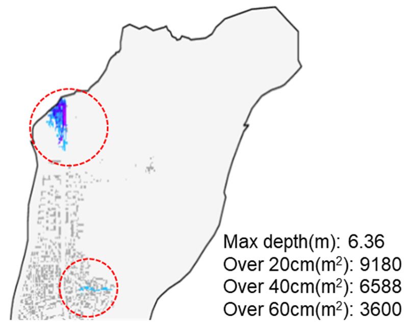
Remote Sens. 2019, 11, 642                                                                                           7 of 19

    Remote Sens. 2019, 1, x FOR PEER REVIEW                                                                    7 of 19
represent typical occurrences of heavy rainfall in summer in Seoul, especially with regard to the flood
damage
    Case caused
          3. After aby1hheavy   rainfall
                          lead time,      that actually
                                     all three          occurred
                                               QPFs differed          in Case
                                                               in rainfall       3.
                                                                            intensity   from the corresponding QPE,
     Figure
    but  their4spatial
                 compares     quantitative
                         distribution         precipitation
                                       was similar.   However, estimates
                                                                   after a 2(QPE,
                                                                               h lead from   theallKMA
                                                                                         time,       three Rainrate system)
                                                                                                           QPFs clearly
withdiffered
      MAPLE,      KONOS,
               from  the QPEand    SCDMdistribution
                                in spatial  rainfall dataas generated      withFigure
                                                             well. Similarly,     1–3 h lead    times starting
                                                                                          5 compares     QPE dataatwith
                                                                                                                    09:20 in
CaseNWP    rainfall
      3. After   a1h data
                       leadgenerated
                             time, allwith
                                        three1–3 h lead
                                               QPFs      times in
                                                     differed    starting  at intensity
                                                                    rainfall   09:00 in Case
                                                                                           from3.the
                                                                                                   Thecorresponding
                                                                                                         NWP data alsoQPE,
but their spatial distribution was similar. However, after a 2 h lead time, all three QPFstoclearly
    show    different  rainfall distributions  and  intensities   for  each  lead   time,  which    seems     be duediffered
                                                                                                                      to
    differences   in the prediction  methods.
from the QPE in spatial distribution as well. Similarly, Figure 5 compares QPE data with NWP rainfall
          Since the
data generated        variability
                    with           of predicted
                           1–3 h lead             rainfall
                                       times starting   at is09:00
                                                               rather   large, 3.due
                                                                    in Case        ThetoNWP
                                                                                          different
                                                                                                datadataalsosources and
                                                                                                             show different
    forecasting techniques, the accuracy of hydrologic forecasting is strongly influenced by which rainfall
rainfall distributions and intensities for each lead time, which seems to be due to differences in the
    prediction is used. Therefore, we used various QPFs and blended QPF to evaluate hydrological
prediction methods.
    applicability in this study.

              (a) QPE (10:20)                      (b) QPE (11:20)                     (c) QPE (12:20)

        (d) MAPLE (1 h lead time)             (e) MAPLE (2 h lead time)          (f) MAPLE (3 h lead time)

        (g) KONOS (1 h lead time)             (h) KONOS (2 h lead time)          (i) KONOS (3 h lead time)

         (j) SCDM (1 h lead time)             (k) SCDM (2 h lead time)            (l) SCDM (3 h lead time)

           Figure 4. Comparison between actual quantitative precipitation estimates (QPE, a–c) and QPF
      Figure   4. Comparison between actual quantitative precipitation estimates (QPE, a–c) and QPF forecasts
           forecasts by the radar-based McGill Algorithm for Prediction Nowcasting by Lagrangian
      by the radar-based McGill Algorithm for Prediction Nowcasting by Lagrangian Extrapolation (MAPLE)
           Extrapolation (MAPLE) (d–f), KOrea NOwcasting System (KONOS) (g–i), and Spatial-scale
      (d–f), KOrea NOwcasting System (KONOS) (g–i), and Spatial-scale Decomposition method (SCDM)
      (j–l) models in the Seoul area with lead times of 1–3 h starting from 09:20, 5 July 2016.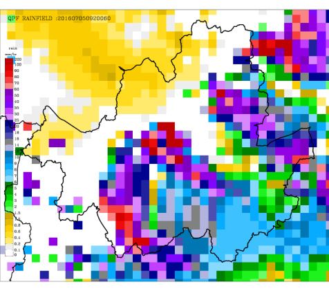
Remote Sens. 2019, 1, x FOR PEER REVIEW                                                                    8 of 19

Remote Sens. 2019, 11, 642 method (SCDM) (j–l) models in the Seoul area with lead times of 1–3 h starting from 8 of 19
        Decomposition
        09:20, July 5, 2016.

            (a) QPE (10:00)                      (b) QPE (11:00)                     (c) QPE (12:00)

    (d) UM LDAPS (1 h lead time)        (e) UM LDAPS (2 h lead time)         (f) UM LDAPS (3 h lead time)

      (g) ASAPS (1 h lead time)             (h) ASAPS (2 h lead time)          (i) ASAPS (3 h lead time)

       Figure
     Figure     5. Comparison
             5. Comparison      between
                             between      actual
                                      actual     quantitative
                                             quantitative      precipitation
                                                          precipitation      estimates
                                                                        estimates (QPE, (QPE,
                                                                                        a–c) anda–c) and
                                                                                                   QPF    QPF
                                                                                                       forecasts
     byforecasts  by the numerical
        the numerical              weather prediction
                          weather prediction  (NWP) (NWP)
                                                       modelsmodels
                                                               UnifiedUnified
                                                                         ModelModel
                                                                                LocalLocal
                                                                                       DataData   Assimilation
                                                                                              Assimilation  and
       and Prediction (UM LDAPS) (d–f) and Advanced Storm-scale Analysis and Prediction System
     Prediction (UM LDAPS) (d–f) and Advanced Storm-scale Analysis and Prediction System (ASAPS)
       (ASAPS) (g–i) in the Seoul area with lead times of 1–3 h starting from 09:00, July 5, 2016.
     (g–i) in the Seoul area with lead times of 1–3 h starting from 09:00, 5 July 2016.

         We evaluated
      Since              the quantitative
             the variability              accuracy
                               of predicted         of is
                                              rainfall three radar-based
                                                          rather          QPFs
                                                                 large, due  to (SCDM,
                                                                                 differentMAPLE,  KONOS),
                                                                                           data sources and
forecasting techniques, the accuracy of hydrologic forecasting is strongly influenced by whichrainfall
   and  the two  NWP    QPFs  (UM   LDAPS,   ASAPS),   along with the blended QPF,   using observed  rainfall
   data from 25 stations in Seoul as the true rainfall. The evaluation was performed every 10 min for
prediction is used. Therefore, we used various QPFs and blended QPF to evaluate hydrological
   lead times from 10–360 min, using RMSE and correlation coefficient (r) as the verification criteria.
applicability in this study.
         The correlation coefficient differed depending on the predicted rainfall type and the QPF update
      We evaluated the quantitative accuracy of three radar-based QPFs (SCDM, MAPLE, KONOS),
   time (Figure 6). The correlation coefficient of the blended QPF was better than those of the other QPFs
and the two NWP QPFs (UM LDAPS, ASAPS), along with the blended QPF, using observed rainfall
   at the time of maximum rainfall in Case 1, but in Cases 2 and 3 this was higher than that of NWP QPF
data from 25 stations in Seoul as the true rainfall. The evaluation was performed every 10 min for lead
   but lower than that of the radar-based QPFs. Although the blended QPF did not always have the
times from 10–360 min, using RMSE and correlation coefficient (r) as the verification criteria.
   highest correlation coefficient, its accuracy variation was not as large as those of the other QPFs due
   to The  correlation
      the merging       coefficient differed depending on the predicted rainfall type and the QPF update
                    effect.
time (Figure 6). The correlation coefficient of the blended QPF was better than those of the other QPFs
at the time of maximum rainfall in Case 1, but in Cases 2 and 3 this was higher than that of NWP QPF
but lower than that of the radar-based QPFs. Although the blended QPF did not always have the
highest correlation coefficient, its accuracy variation was not as large as those of the other QPFs due to
the merging effect.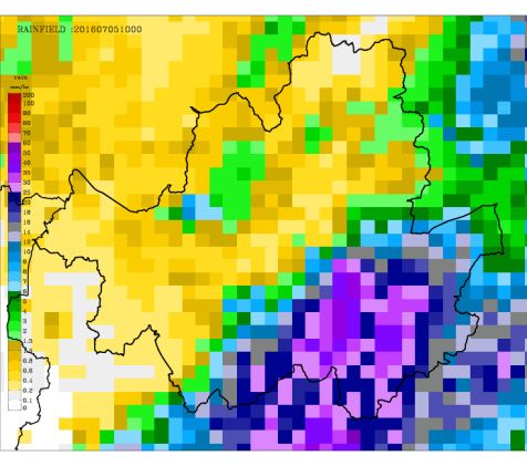
Remote Sens. 2019, 11, 642 9 of 19
Remote Sens. 2019, 1, x FOR PEER REVIEW 9 of 19
Remote Sens. 2019, 1, x FOR PEER REVIEW 9 of 19
(a) Case 1 (1 July 2016, 14:00–1500) (b) Case 2 (1 July 2016, 15:00–23:50)
(a) Case 1 (1 July 2016, 14:00–1500) (b) Case 2 (1 July 2016, 15:00–23:50)
(c) Case 3 (5 July 2016, 09:10–10:50)
Figure
(c)6.
Figure Accuracy
6.Case evaluations
3 (5 July
Accuracy (by
(by correlation
correlation coefficient)
2016, 09:10–10:50)
evaluations coefficient) for
for real-time
real-time QPF
QPF produced
produced byby the
the five
five
tested
tested models
models and and the
the blended
blended approach
approach for
for all
allthree
threecases.
cases.Grey
Greyline
linemarks
markspeak
peakactual
actualprecipitation.
precipitation.
Figure 6. Accuracy evaluations (by correlation coefficient) for real-time QPF produced by the five
(a)
(a) Case
Case 1;
1; (b)
(b) Case
Case 2;
2; (c)
(c) Case
Case 33
tested models and the blended approach for all three cases. Grey line marks peak actual precipitation.
(a) Case 1; (b) Case 2; (c) Case 3
The RMSE
The RMSEfor forall
allQPFs
QPFsbecame
becamesmaller
smalleroverover time
time (Figure
(Figure 7).7).
AsAs thethe analysis
analysis periods
periods ran ran
fromfrom
the
the beginning
beginning toend
to the theof
end of precipitation,
precipitation, the RMSEthe RMSE naturally
naturally declineddeclined
due to due to the smaller
the smaller amountamount of
of rainfall
The RMSE for all QPFs became smaller over time (Figure 7). As the analysis periods ran from the
rainfall
at at termination.
termination. Therefore, Therefore,
we analyzedwe analyzed errorsthe
errors between between the QPFs
QPFs relative relative
to the to the computation
computation time rather
beginning to the end of precipitation, the RMSE naturally declined due to the smaller amount of rainfall
than as the than
time rather absolute
as theRMSE at each
absolute RMSE computation time. Thetime.
at each computation RMSE TheofRMSE
the ASAPS QPF had
of the ASAPS QPFlarger
had
at termination. Therefore, we analyzed errors between the QPFs relative to the computation time rather
fluctuations in Casesin1 and
larger fluctuations Cases2 at
1 each
and 2computation time, while
at each computation the variations
time, while the in RMSE forinthe
variations threefor
RMSE radar-
the
than as the absolute RMSE at each computation time. The RMSE of the ASAPS QPF had larger
based QPFs were similar
three radar-based and not
QPFs were larger
similar than
and notthose
largerof than
the NWP
thoseQPFs.
of theTheNWP RMSEQPFs.of The
the blended
RMSE ofQPF the
fluctuations in Cases 1 and 2 at each computation time, while the variations in RMSE for the three radar-
tended
blendedtoQPFmatch thatto
tended ofmatch
the radar
that based QPFs;based
of the radar in Cases
QPFs; 1 and 2, the1RMSE
in Cases and 2, of
thethe blended
RMSE of theQPF was
blended
based QPFs were similar and not larger than those of the NWP QPFs. The RMSE of the blended QPF
lowest
QPF was at the timeat
lowest ofthe
maximum
time of rainfall
maximum occurrence. Figure 8 shows
rainfall occurrence. the time
Figure seriesthe
8 shows of time
the weights
series ofofthe
all
tended to match that of the radar based QPFs; in Cases 1 and 2, the RMSE of the blended QPF was
models
weightsestimated fromestimated
of all models the HS method
from thefor HS
Case 3; the blended
method for CaseQPF3; theis blended
estimatedQPFusing these weights.
is estimated using
lowest at the time of maximum rainfall occurrence. Figure 8 shows the time series of the weights of all
these weights.
models estimated from the HS method for Case 3; the blended QPF is estimated using these weights.
(a) Case 1 (1 July 2016, 14:00–1500) (b) Case 2 (1 July 2016, 15:00–23:50)
(a) Case 1 (1 July 2016, 14:00–1500) (b) Case 2 (1 July 2016, 15:00–23:50)
(c) Case 3 (5 July 2016, 09:10–10:50)
Figure
(c)7.Case
Accuracy evaluations
3 (5 July (by root mean square error) for real-time QPF produced by the five
2016, 09:10–10:50)
tested models and the blended approach for all three cases. Grey line marks peak actual precipitation.
Figure 7. Accuracy evaluations (by root mean square error) for real-time QPF produced by the five
Case7.1;Accuracy
Figure
(a) (b) Case 2;evaluations
(c) Case 3 (by root mean square error) for real-time QPF produced by the five
tested
tested models and the blended approach for
models and the blended approach for all
all three
three cases.
cases. Grey
Greyline
linemarks
markspeak
peakactual
actualprecipitation.
precipitation.
(a)
(a) Case 1; (b)
Case 1; (b) Case
Case 2;
2; (c)
(c) Case
Case 33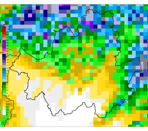
Remote Sens. 2019, 11, 642 10 of 19
Remote
Remote Sens.
Sens. 2019,
2019, 1,
1, xx FOR
FOR PEER
PEER REVIEW
REVIEW 10
10 of
of 19
19
Figure
Figure 8.
8. Time
Time series
series of
of the
the weights of all
weights of all models
models estimated
estimated from
from the
the HS
HS method
method for
for Case
Case 3.
3.
3.2.
3.2. Analysis
Analysis of
of Real-Time
Real-Time Urban
Urban Runoff
Runoff Forecasting
Forecasting Using
Using QPFs
QPFs
We used the
We used theSWMM
SWMMto to perform
perform real-time
real-time urban
urban runoff
runoff forecasting
forecasting using using the radar-based,
the radar-based, NWP-
NWP-based, and blended QPFs to assess the hydrological applicability of using QPF.
based, and blended QPFs to assess the hydrological applicability of using QPF. The two study areas,The two study
areas,
in the inGangnam
the Gangnam and Bakwoon
and Bakwoon basins,
basins, are are locations
locations where
where inundationand
inundation andoverflow
overflowoften
often occur
(Figure
(Figure 9). The SWMM input of the Gangnam drainage system comprises 1059 pipes, 773 manholes,
9). The SWMM input of the Gangnam drainage system comprises 1059 pipes, 773 manholes,
and 2 area.
and 772
772sub-basins
sub-basinsover
overa 7.4 kmkm
a 7.4 Water
22 area. depth
Water in pipe
depth in was
piperecorded at threeatobservation
was recorded stations
three observation
for evaluation.
stations The Bakwoon
for evaluation. basin testbasin
The Bakwoon is discussed in Section
test is discussed in3.3.
Section 3.3.
(a) Gangnam basin (b) Bakwoon basin
Figure 9.
Figure 9. Drainage
Drainage system
system used
used in
in Storm
Storm Water
Water Management
Management Model
Model (SWMM)
(SWMM) assessments
assessments of
of the
the (a)
(a)
Gangnam basin and (b) Bakwoon basin (Section 3.3).
Gangnam basin and (b) Bakwoon basin (Section 3.3).
The three
three previously
previouslydefined
definedcases
caseswere
wereused
usedforfor evaluation
evaluation of of urban
urban runoff
runoff forecasting
forecasting withwith
the
the rainfall
rainfall inputinput forSWMM
for the the SWMM model model produced
produced by QPEby and
QPEQPF andat QPF
each atcurrent
each current timefor
time (CT) (CT)
3 hfor 3h
ahead
ahead
of of forecast.
forecast. FigureFigure 10 compares
10 compares the observed
the observed and simulated
and simulated depthsdepths
using using
all QPFsall QPFs for 1Case
for Case from1
from 14:00–15:50.
14:00–15:50. The ASAPS
The ASAPS QPF effectively
QPF effectively simulated
simulated the peak thewater
peak water
depth depth occurrence
occurrence time andtime and
water
water depth
depth change change patterns.
patterns. In addition,
In addition, the blended
the blended QPFQPF showed
showed the the second-best
second-best simulation
simulation results
results at
at 15:30
15:30 andand 15:50.
15:50. The
The radar-basedand
radar-based andUMUMLDASLDASQPFsQPFscould
couldnot notaccurately
accuratelysimulate
simulate thethe peak
peak flow
showed significantly
and showed
and significantlylower
lowersimulated
simulatedsewer
sewer water
water depths.
depths. Statistical
Statistical evaluations
evaluations showed
showed thatthat
the
the relative
relative errorerror of peak
of peak depth depth
(REPD)(REPD) for ASAPS
for ASAPS was thewas the lowest
lowest (−19.11%(−19.11% to 11.66%)
to 11.66%) of all while
of all QPFs QPFs
while RMSE
RMSE for thefor the blended
blended modelmodel was lowest
was lowest (0.33–0.38)
(0.33–0.38) (Table (Table
1). 1).Remote Sens. 2019, 11, 642 11 of 19
Remote Sens. 2019, 1, x FOR PEER REVIEW 11 of 19
(a) 15:00 (b) 15:30
(c) 15:50
Figure
Figure 10.
10. Comparisons
Comparisonsbetween
betweenobserved
observedand andsimulated
simulatedrainfall
rainfalldata using
data usingwater
water depth in in
depth pipe at
pipe
three locations
at three in in
locations Gangnam
Gangnam forfor
Case
Case1 1(July 1, 2016)
(1 July 2016)over
over time.
time. Upper
Uppergraphs
graphs are
are the
the mean
mean area
area
precipitation
precipitation forecasted
forecasted by
by each
each QPF
QPF (lines)
(lines) and
and the
the actual
actual AWS data (grey
AWS data (grey bars).
bars). Lower
Lower graphs
graphs are
are
simulated (lines) and observed (circles) water depth in pipe. Vertical grey lines mark the current
simulated (lines) and observed (circles) water depth in pipe. Vertical grey lines mark the current time time
of
of each
each subfigure.
subfigure. (a)
(a) 15:00;
15:00; (b)
(b) 15:30;
15:30; (c)
(c) 15:50
15:50.
Figure 11 compares results for Case 2 at at 21:00,
21:00, 21:30,
21:30, and
and 22:00.
22:00. The blended QPF accurately
simulated the peak water depth occurrence time and water water depth
depth change
change patterns.
patterns. When rainfall
decreased, the NWP-based
NWP-based QPF was overestimated and affected the overestimate of the blended
predicted rainfall. On the other
other hand,
hand, the
the radar-based
radar-based QPFs
QPFs were
were underestimated
underestimated at at all
allcurrent
currenttimes.
times.
Statistically, theblended
Statistically, the blendedQPF
QPFhad
hadthe
thelowest
lowestREPD
REPDandandRMSE
RMSEininCase
Case2,2,ranging from−−14.0
rangingfrom to−
14.0 to −27.08
27.08
and 0.31–0.60, respectively
respecti (Table 2).
vely (Table 2).Remote Sens. 2019, 11, 642 12 of 19
Remote Sens. 2019, 1, x FOR PEER REVIEW 12 of 19
(a) CT 1 July 2016 21:00 (b) CT 1 July 2016 21:30
(c) CT 1 July 2016 22:00
Figure 11.
Figure 11. Comparisons
Comparisons between
between observed
observed and
and simulated
simulated rainfall
rainfall data
data using
using water
water depth
depth in
in pipe
pipe at
at
three locations in Gangnam for Case 2 (July 1, 2016) over time.
three locations in Gangnam for Case 2 (1 July 2016) over time.
Figure12
Figure 12compares
comparesresults
resultsforfor Case
Case 3 at
3 at 09:20,
09:20, 09:30,
09:30, andand 09:40.
09:40. TheThe blended
blended QPFQPF
and and
ASAPSASAPS
had
had higher
higher accuracy
accuracy than than
thosethose the other
the other QPFsQPFs in terms
in terms of peakof water
peak water
depthdepth occurrence
occurrence timepeak
time and and
peak water depth. In particular, since the merged QPF is affected by the radar QPF (updated
water depth. In particular, since the merged QPF is affected by the radar QPF (updated every 10 min), every
it10follows
min), itthe
follows the temporal
temporal variation variation of the
of the rainfall rainfall
more thanmore than thewhich
the ASAPS, ASAPS, whichevery
updates updates every
hour. All
hour. All evaluation
evaluation indicators indicators
showed good showed good
results for results
blendedfor blended
QPF (TableQPF
3). (Table 3).Remote Sens. 2019, 11, 642 13 of 19
Remote Sens. 2019, 1, x FOR PEER REVIEW 13 of 19
(a) CT 5 July 2016 09:20 (b) CT 5 July 2016 09:30
(c) CT 5 July 2016 09:40
Figure 12.
Figure 12. Comparisons
Comparisons between
between observed
observed and
and simulated
simulated rainfall
rainfall data
data using
using water
water depth
depth in
in pipe
pipe at
at
three locations in Gangnam for Case 3 (July 5, 2016) over time.
three locations in Gangnam for Case 3 (5 July 2016) over time.Remote Sens. 2019, 11, 642 14 of 19
Table 1. Evaluation results for simulated water depth using various QPF products (Case 1) in terms of correlation coefficient (r), relative error of peak depth (REPD),
and root mean square error (RMSE) by current time (CT).
AWS MAPLE KONOS SCDM UM ASAPS BLENDED
CT
r RMSE REPD r RMSE REPD r RMSE REPD r RMSE REPD r RMSE REPD r RMSE REPD r RMSE REPD
15:00 0.63 0.32 −0.71 −0.30 0.49 −84.67 −0.20 0.49 −83.37 0.59 0.37 −42.60 −0.56 −0.55 −76.51 0.32 0.49 0.65 0.51 0.36 −62.89
15:30 0.57 0.34 1.42 0.40 0.48 −64.70 0.44 0.47 −60.77 0.42 0.44 −54.20 −0.58 −0.58 −76.15 0.14 0.51 −19.11 0.40 0.38 −34.79
15:50 0.80 0.22 2.78 0.42 0.41 −8.52 0.52 0.36 14.55 0.55 0.35 −0.89 0.37 −0.36 −0.83 0.21 0.47 11.66 0.48 0.33 −2.07
Table 2. Evaluation results for simulated water depth using various QPF products (Case 2) in terms of correlation coefficient (r), relative error of peak depth (REPD),
and root mean square error (RMSE) by current time (CT).
AWS MAPLE KONOS SCDM UM ASAPS BLENDED
CT
r RMSE REPD r RMSE REPD r RMSE REPD r RMSE REPD r RMSE REPD r RMSE REPD r RMSE REPD
21:00 0.76 0.34 −6.67 0.40 0.67 −65.03 0.30 0.61 −65.03 0.47 0.65 −65.02 −0.57 0.79 −12.51 0.68 0.79 35.08 0.01 0.50 −27.08
21:30 0.82 0.32 2.41 0.49 0.56 −55.54 0.60 0.48 −53.44 0.62 0.51 −54.00 −0.61 0.90 −10.05 0.80 0.73 38.05 0.83 0.31 −15.79
22:00 0.87 0.28 −7.64 0.98 0.35 −45.44 0.87 0.32 −43.79 0.98 0.37 −47.18 −0.06 0.88 −10.56 −0.12 1.02 15.38 0.51 0.60 −14.00
Table 3. Evaluation results for simulated water depth using various QPF products (Case 3) in terms of correlation coefficient (r), relative error of peak depth (REPD),
and root mean square error (RMSE) by current time (CT).
AWS MAPLE KONOS SCDM UM ASAPS BLENDED
CT
r RMSE REPD r RMSE REPD r RMSE REPD r RMSE REPD r RMSE REPD r RMSE REPD r RMSE REPD
9:20 0.94 0.22 −2.00 0.81 0.53 −59.39 0.89 0.55 −63.22 0.83 0.48 −61.67 0.89 0.58 −67.11 0.89 0.33 −24.50 0.92 0.26 −15.83
9:30 0.93 0.24 5.78 0.85 0.48 −50.50 0.83 0.46 −34.89 0.90 0.51 −51.50 0.93 0.51 −52.66 0.91 0.30 −28.39 0.94 0.24 −19.11
9:40 0.92 0.25 0.44 0.92 0.47 −53.78 0.83 0.43 −30.11 0.92 0.54 −55.11 0.93 0.46 −51.39 0.93 0.27 −25.56 0.95 0.20 −8.67Remote Sens. 2019, 1, x FOR PEER REVIEW 14 of 19
3.3. Analysis of Real-time Urban Inundation Forecasting Using QPFs
RemoteWe
Sens.analyzed
2019, 11, 642the effects of all tested QPFs by forecasting inundation in an urban area 15using of 19
existing
Remote information
Sens. 2019, 1, x FORfor July
PEER 5, 2016, an event that caused actual flood damage in the Bakwoon
REVIEW 14 area.
of 19
Inundated areas included the Surak underpass structure and the Sanggye-dong multiplex houses
3.3. Analysis of Real-time Urban Inundation Forecasting Using QPFs
(Figure 13). The inundation information consisted of digital photos taken at the inundation sites. The
3.3. Analysis of Real-time Urban Inundation Forecasting Using QPFs
SWMM We model
analyzed wasthe seteffects
up as of all tested
shown QPFs9bbywith
in Figure forecasting
input data inundation
from 1163inmanholes,
an urban 1125
area pipes,
using
existing
We information
and 1081 analyzed
sub-basins theforeffects
over 5 aJuly
9.1of2016,
km an event
all2 area.
tested
The thatby
QPFs
GIAM caused actual
forecasting
was then flood damage
setinundation
up with in in
anthe
a spatial Bakwoon
urban area of
resolution area.
using
6m
Inundated
existing
and a time areas included
information
interval offor July
0.05 the5, Surak
s. 2016, an underpass structure
event that and the
caused actual Sanggye-dong
flood damage in the multiplex
Bakwoon houses
area.
(Figure
Inundated13).areas
Figure The
14 inundation
included
shows theinformation
the surcharge Surak flow consisted
underpass
from of digital
thestructure
manhole and
wherephotos
thethe taken at the
Sanggye-dong
maximum inundation
multiplex
amount sites.
houses
of overflow
The SWMM
(Figure 13). model
The was
inundation set up as shown
information in Figure
consisted 9b
of with input
digital data
photos from
taken 1163
at
occurred (red star of Figure 12) as simulated by all QPFs and AWSs. As there was no water depth the manholes,
inundation 1125 pipes,
sites. The
and 1081model
sub-basins over 2
SWMM
observation was in
station set upaBakwoon
the 9.1shown
as km area. The
weGIAM
in Figure
basin, wasinput
9b with
compared then data
set up
simulated with1163
from a spatial
surcharge flow resolution
manholes, AWSof
using1125 6m
pipes,
data.
and
The ablended
timesub-basins
1081 interval
modelof 0.05
mostas.similar
isover 9.1 km2to area. The gauge
the rain GIAM data
was in
then set of
terms uppeak
withsurcharge
a spatial resolution of 6 m
flow and timing.
and a time interval of 0.05 s.
Figure 14 shows the surcharge flow from the manhole where the maximum amount of overflow
occurred (red star of Figure 12) as simulated by all QPFs and AWSs. As there was no water depth
observation station in the Bakwoon basin, we compared simulated surcharge flow using AWS data.
The blended model is most similar to the rain gauge data in terms of peak surcharge flow and timing.
Bakwoon basin.
Figure 13. Actual flooding locations in the Bakwoon basin.
Figure 14 shows the surcharge flow from the manhole where the maximum amount of overflow
occurred (red star of Figure 12) as simulated by all QPFs and AWSs. As there was no water depth
observation station in the Bakwoon basin, we compared simulated surcharge flow using AWS data.
The blended model is most similar
Figure to theflooding
13. Actual rain gauge data in
locations inthe
terms of peak
Bakwoon surcharge flow and timing.
basin.
Figure 14. Surcharge flows simulated by the SWMM using various QPFs (lines) and AWS rainfall data
(circles). Current time is marked by vertical dashed line.
Figure 15 shows the maximum inundation maps for AWS data and each QPF, which are
noticeably different. Because no observed inundation map exists, only photos, the accuracy
comparison
Figure 14. for the inundation
Surcharge forecasting
flows simulated by the is basedusing
SWMM on simulation
various QPFs results
(lines) from
and AWSthe rainfall
AWS-observed
data
rainfall. MAPLE
(circles).
(circles). is significantly
Current time is
time is marked
markedunderestimated
by vertical
by inundation
vertical dashed
dashed line.
line. while the ASAPS and UM LDAPS results
were similar to AWS result. The radar-based and NWP QPFs all predicted flooding only at the Surak
Figure
underpass 1515shows
Figurestructure.
shows the maximum
the
The maximum
blended inundation
QPF inundationmapswas
simulation for most
maps AWS data
AWSand
for similar toeach
data QPF,
theand which
each
observed are which
QPF,
spatial noticeably
extentare
of
different.
noticeably Because
different.
flood inundation no observed
and Because
was inundation
no model
the only tomap
observed exists,
inundation
predict onlymap
flooding photos, the accuracy
exists,
at the comparison
only photos,
Sanggye-dong for the
the accuracy
multiplex houses.
inundation
comparison forecasting is based forecasting
for the inundation on simulation results
is based onfrom the AWS-observed
simulation results from rainfall. MAPLE is
the AWS-observed
significantly
rainfall. MAPLE underestimated
is significantly inundation while theinundation
underestimated ASAPS andwhile UM LDAPS
the ASAPS results
andwere
UM similar
LDAPStoresults
AWS
result. The radar-based
were similar to AWS result. and The
NWP QPFs all predicted
radar-based and NWP flooding
QPFs all only at the Surak
predicted floodingunderpass
only at thestructure.
Surak
The blended
underpass QPF simulation
structure. was most
The blended QPF similar to the
simulation was observed spatialtoextent
most similar of flood spatial
the observed inundation and
extent of
was the only model to predict flooding at the Sanggye-dong multiplex houses.
flood inundation and was the only model to predict flooding at the Sanggye-dong multiplex houses.Remote Sens. 2019, 11, 642 16 of 19
Remote Sens. 2019, 1, x FOR PEER REVIEW 15 of 19
(a) AWS (b) MAPLE
(c) KONOS (d) SCDM
(e) UM LDAPS (f) ASAPS
(g) Blended QPF
Figure15.
Figure 15.Maximum
Maximum inundation
inundation maps
maps produced
produced using
using various
various QPFs
QPFs and
and AWS
AWS data.
data.Remote Sens. 2019, 11, 642 17 of 19
The forecasting results showed a maximum inundation depth for the blended QPF of 6.36 m, close
to the AWS result (6.70 m) (Table 4). For the AWS result, the inundated area exceeding 20 cm depth
was 11,376 m2 and the blended result was a similar 9180 m2 . The inundated areas of the other QPFs
were much smaller than the AWS result. For the inundated area exceeding 40 cm, all QPF results were
considerably smaller than the AWS result; the blended QPF’s inundated area was 6588 m2 , about 40%
smaller than the AWS result. These results confirm the usefulness of the blended QPF approach for
urban flood forecasting. However, future research should consider the data period used for blending
the weight and production time of the forecasting model, considering the influence of past forecast
errors when estimated the blending weights and the influence of different forecasting techniques.
Table 4. Inundation forecast results in terms of max depth and inundated area for each criterion.
Criteria AWS MAPLE KONOS SCDM UM ASAPS BLENDED
Max Depth (m) 6.70 4.49 5.81 6.45 6.10 6.05 6.36
Inundated area over 20 cm (m2 ) 11,376 144 2376 7596 5148 4068 9180
Inundated area over 40 cm (m2 ) 11,268 72 1512 5328 3600 3888 6588
Inundated area over 60 cm (m2 ) 9036 36 360 3600 4248 3240 3600
4. Conclusions
In this study, we developed a new real-time adaptive blending technique using the harmony
search algorithm to improve the accuracy of rainfall forecasts for hydrological applications. Three
radar-based QPFs (MAPLE, KONOS, and SCDM) and two NWP QPFs (UM LDAPS and ASAPS)
were used for the blending process. We also assessed the hydrological applicability of the individual
and blended QPFs for use in urban flood forecasting in Seoul, South Korea. Our proposed blended
approach was based on the assumption that the error of the previously predicted rainfall was similar
to that of current predicted rainfall. Using the harmony search algorithm, we optimized real-time
weights that would minimize the root mean square error between predicted and observed rainfall for
a 1 h lead time at 10 min intervals.
Our accuracy analysis using the six QPFs with three real-life rainfall cases showed that the
blended QPF could be calculated with stable accuracy. The SWMM and GIAM models were then used
to estimate urban flood discharge and to forecast the inundated area using rainfall from the QPFs
and AWS data. Although the blended QPF did not always have the highest correlation coefficient, its
accuracy varied less than that of the other QPFs. In addition, its simulated water depth in pipe and
spatial extent were most similar to observed inundated areas, demonstrating the value of this new
blending approach for short-term flood forecasting. When comparing the inundated areas from AWS
data, the predicted inundated areas showed that the blended forecast could more accurately simulate
actual inundated locations than any other QPFs.
Our results were limited by the generalized nature of the study, as it assessed the blending
technique using only a few rainfall cases in a specific area. However, the improved accuracy of the
blended QPF is quite meaningful with regard to this approach’s hydrological applicability in cases of
extreme rainfall. Future research should build on these results by assessing more diverse rainfall cases
and study areas. In addition, we intend to further optimize the weights using various storm events
and criteria while working to improve the prediction accuracy using a spatial blending technique.
Author Contributions: Experiment, data analysis, and writing/revision of the manuscript, S.-S.Y.
Funding: This research was funded by the KICT Strategic Research Project (Development of Driving Environment
Observation, Prediction and Safety Technology Based on Automotive Sensors).
Conflicts of Interest: The authors declare no conflict of interest.
References
1. Daley, R. Atmospheric Data Analysis; Cambridge University Press: Cambridge, UK, 1991; p. 457.Remote Sens. 2019, 11, 642 18 of 19
2. Golding, B.W. Long lead time flood warnings: Reality or fantasy? Meteorol. Appl. 2009, 16, 3–12. [CrossRef]
3. Golding, B.W. Nimrod: A system for generating automated very short range forecasts. Meteorol. Appl.
1998, 5, 1–16. [CrossRef]
4. Pierce, C.E.; Hardaker, P.J.; Collier, C.G.; Haggett, C.M. GANDOLF: A system for generating automated
nowcasts of convective precipitation. Meteorol. Appl. 2000, 7, 341–360. [CrossRef]
5. Wong, W.K.; Lai, E.S.T. RAPIDS—Operational Blending of Nowcast and NWP QPF. In Proceedings of the
2nd International Symposium on Quantitative Precipitation Forecasting and Hydrology, Boulder, CO, USA,
4–8 June 2006.
6. Bowler, N.E.; Pierce, C.E.; Seed, A.W. STEPS: A probabilistic precipitation forecasting scheme which merges
an extrapolation nowcast with downscaled NWP. Q. J. R. Meteorol. Soc. 2006, 132, 2127–2155. [CrossRef]
7. Wong, W.K.; Yeung, L.; Wang, Y.C.; Chen, M.X. Towards the blending of NWP with nowcast: Operation
experience in B08FDP. In Proceedings of the World Weather Research Program Symposium on Nowcasting,
Whistler, BC, Canada, 30 August–4 Sepetember 2009.
8. Lin, C.; Vasic, S.; Kilambi, A.; Turner, B.; Zawadzki, I. Precipitation forecast skill of numerical weather
prediction models and radar nowcasts. Geophys. Res. Lett. 2005, 32, L14801. [CrossRef]
9. Ebert, E.; Seed, A. Use of radar rainfall estimates to evaluate mesoscale model forecasts of convective
rainfall. In Proceedings of the Sixth International Symposium on Hydrological Applications of Weather
Radar, Melbourne, Australia, 2–4 February 2004; pp. 271–273.
10. Kilambi, A.; Zawadzki, I. An evaluation of ensembles based upon MAPLE precipitation nowcasts and NWP
precipitation forecasts. In Proceedings of the 32nd Conference on Radar Meteorology, Albuquerque, Mexico,
24–29 October 2005.
11. Wilson, J.; Xu, M. Experiments in blending radar echo extrapolation and NWP for nowcasting convective
storms. In Proceedings of the Fourth European Conference on Radar in Meteorology and Hydrology,
Barcelona, Spain, 18–22 September 2006; pp. 519–522.
12. Pinto, J.; Mueller, C.; Weygandt, S.; Ahijevych, D.; Rehak, N.; Megenhardt, D. Fusion observation- and
model-based probability forecasts for the short term prediction of convection. In Proceedings of the 12th
Conference on Aviation, Range, and Aerospace Meteorology, Atlanta, Georgia, 30 January–2 February 2006.
13. Golding, B.W. Quantitative precipitation forecasting in the UK. J. Hydrol. 2000, 239, 286–305. [CrossRef]
14. Atencia, A.; Rigo, T.; Sairouni, A.; More, J.; Bech, J.; Vilacara, E.; Cunillera, J.; Llasat, M.C.; Garrote, L.
Improving QPF by blending techniques at the Meteorological Service of Catalonia. Nat. Hazards Earth
Syst. Sci. 2010, 10, 1443–1455. [CrossRef]
15. Yoon, S.S. Development of radar-based quantitative precipitation forecasting using spatial-scale
decomposition method for urban flood management. J. Korea Water Resour. Assoc. 2017, 50, 335–346.
16. Laroche, S.; Zawadzki, I. A variational analysis method for the retrieval of three-dimensional wind field
from single Doppler radar data. J. Atmos. Sci. 1994, 53, 2664–2682. [CrossRef]
17. Germann, U.; Zawadzki, I. Scale dependence of the predictability of precipitation from continental radar
images. Part I: Description of the methodology. Mon. Weather Rev. 2002, 130, 2859–2873. [CrossRef]
18. Germann, U.; Zawadzki, I.; Turner, B. Predictability of precipitation from continental radar images. Part IV:
Limits to prediction. J. Atmos. Sci. 2006, 63, 2092–2108. [CrossRef]
19. Jin, J.; Lee, H.C.; Ha, J.C.; Lee, Y.H. Development of a nowcasting system combined variational echo
tracking and radar-AWS rainrate composition. Conference of Korean Meteorological Society, Busan, Korea,
26 October 2011; p. 164.
20. Kim, S.H.; Kim, H.M.; Kay, J.K.; Lee, S.W. Development and evaluation of the High Resolution Limited Area
Ensemble Prediction System in the Korea Meteorological Administration Atmosphere. Korean Meteorol. Soc.
2015, 25, 67–83.
21. National Institute of Meteorological Sciences. Development of the Advanced Storm-Scale Analysis and
Prediction System; Technical Report, Korea, NIMR-TN-2014-023; National Institute of Meteorological Sciences:
Seogwipo-si, Korea, 2014. (In Korean)
22. Yoon, S.S.; Lee, B.J. Effects of using high-density rain gauge networks and weather radar data on urban
hydrological analyses. Water 2017, 9, 931. [CrossRef]
23. Jo, D.J. Application of the urban flooding forecasting by the flood nomograph. J. Korean Soc. Hazard Mitig.
2014, 14, 421–425. [CrossRef]Remote Sens. 2019, 11, 642 19 of 19
24. Moon, Y.I.; Kim, J.S. Reducing the Risk of Floods in Urban Areas with Combined Inland-River System. CUNY
Academic Works. 2014. Available online: http://academicworks.cuny.edu/cc_conf_hic/370 (accessed on
1 January 2019).
25. Geem, Z.W.; Kim, J.H.; Loganathan, G.V. A new heuristic optimization algorithm: Harmony search.
Simulation 2001, 76, 60–68. [CrossRef]
26. Perelman, L.; Ostfeld, A. Optimal cost design of water distribution networks using harmony search.
Eng. Optim. 2007, 39, 259–277. [CrossRef]
27. Geem, Z.W. State-of-the-art in the structure of harmony search algorithm. Stud. Comput. Intell. 2010, 270,
1–10. [CrossRef]
28. Geem, Z.W. Parameter Estimation of the Nonlinear Muskingum Model Using Parameter-Setting-Free
Harmony Search. J. Hydrol. Eng. 2011, 16, 684–688. [CrossRef]
29. Huber, W.C.; Heaney, J.P.; Nix, S.J.; Dickinson, R.E.; Polmann, D.J. Storm Water Management Model User’s
Manual Version III; EPA-600/2-84-109a; US Environmental Protection Agency: Cincinnati, OH, USA,
1984; p. 504.
30. Huber, W.C.; Dickinson, R.E. Storm Water Management Model, Version 4: Users Manual; US Environmental
Protection Agency, 600/3-88/001a; Environmental Research Laboratory, EPA: Athens, Greece, 1988.
31. Lee, B.J.; Yoon, S.S. Development of grid based inundation analysis model (GIAM). J. Korea Water
Resour. Assoc. 2017, 50, 181–190.
© 2019 by the author. Licensee MDPI, Basel, Switzerland. This article is an open access
article distributed under the terms and conditions of the Creative Commons Attribution
(CC BY) license (http://creativecommons.org/licenses/by/4.0/).You can also read


