SITE EFFECTS ON LARGE GROUND MOTIONS AT KIK-NET IWASE STATION IBRH11 DURING THE 2011 TOHOKU EARTHQUAKE
←
→
Page content transcription
If your browser does not render page correctly, please read the page content below
Bulletin of the Seismological Society of America, Vol. 104, No. 2, pp. 653–668, April 2014, doi: 10.1785/0120130095

                Site Effects on Large Ground Motions at KiK-net Iwase
                 Station IBRH11 during the 2011 Tohoku Earthquake
                  by Toshimi Satoh, Takashi Hayakawa, Mitsuki Oshima, Hiroshi Kawase,
                        Shinichi Matsushima, Fumiaki Nagashima, and Koki Tobita

                Abstract      Large horizontal ground motions with peak ground accelerations (PGAs)
                of more than 800 cm=s2 and peak ground velocities of nearly 60 cm=s were observed
                at a KiK-net station, Iwase (IBRH11), during the 2011 Mw 9.0 Tohoku, Japan, earth-
                quake. We investigated site effects on the large ground motions by inverting the sub-
                surface structure and simulating ground motions considering soil nonlinearity. The
                structure from the seismic bedrock to the surface in the linear regime was inverted
                from (1) array records of microtremors using Rayleigh-wave inversion, (2) surface-
                to-borehole spectral ratios of weak motions using S-wave inversion based on the 1D
                wave propagation theory, and (3) horizontal-to-vertical spectral ratios of weak mo-
                tions using the inversion based on the diffuse-field theory for plane waves. The main
                cause of the large ground motions was found to be a strong impedance contrast be-
                tween soft layers with an S-wave velocity (V S ) of less than 381 m=s and a layer with
                V S  2371 m=s at a depth of 30 m. The strong motions at the surface during the 2011
                Tohoku earthquake simulated by equivalent-linear analysis using borehole records at a
                depth of 103 m are in reasonable agreement with the observed records, whereas those
                simulated using linear analysis were approximately twice as large as the observed
                values. The results showed that the nonlinearity of the surface soils reduced the
                amplification factors and the PGAs by half compared with the values for the linear
                regime. The PGAs of the bedrock motions with V S  2371 m=s were estimated, using
                equivalent-linear analysis, to have reached approximately 500 cm=s2.

                        Introduction
     During the 2011 M w 9.0 Tohoku earthquake, strong-                   possible cause of the large ground motions at IBRH11 during
motion data were recorded in at least 2174 stations in Japan              the 2011 Tohoku earthquake.
by public organizations. Of these 2174 stations, 1224 sta-                     In this study, we investigated the cause of the large
tions were K-NET and KiK-net stations installed by National               ground motions at IBRH11 during the 2011 Tohoku earth-
Research Institute for Earth Science and Disaster Prevention              quake by inverting the subsurface structure from the seismic
(NIED). Records at 430 stations were collected by the Japan               bedrock to the surface and simulating the ground motions,
Meteorological Agency (JMA), and the remaining 520 re-                    considering soil nonlinearity. Nonlinearity was seen at several
cords were from local governments. At all the KiK-net sta-                stations during the 2011 Tohoku earthquake (e.g., Bonilla
tions, strong motions were recorded at ground surfaces and                et al., 2011; De Martin et al., 2012; Hayakawa et al., 2012;
in boreholes, typically at depths of 100 or 200 m. The KiK-               Nagashima et al., 2012). Bonilla et al. (2011) showed the
net station IBRH11 in Iwase, Sakuragawa city, Ibaraki pre-                existence of soil nonlinearity at IBRH11 by comparing the
fecture, Japan, at a hypocentral distance of 310 km, was a                surface-to-borehole (H=HB ) spectral ratios of the weak mo-
station with quite large horizontal peak ground accelerations             tions with the strong motions. To predict strong motions, it is
(PGAs) and peak ground velocities (PGVs). The observed                    important to show that the theoretical simulation that consid-
PGA and PGV values at the surface were more than                          ers soil nonlinearity works well quantitatively. Therefore, we
800 cm=s2 and nearly 60 cm=s, respectively. In addition, dur-             simulated the strong motions at the surface during the 2011
ing the M w 7.2 earthquake that occurred on 7 December                    Tohoku earthquake by the equivalent-linear analysis method
2012 near Japan trench, the PGA value was recorded to be                  (Schnabel et al., 1972) using data from borehole records at a
the second largest and the JMA instrumental seismic intensity             depth of 103 m at IBRH11. We also estimated the bedrock
was largest at IBRH11 among 961 K-NET and KiK-net sta-                    motions on the tertiary or older rock using equivalent analysis
tions. These observations suggest that the site response was a            to show the motions at IBRH11 without site effects.

                                                                    653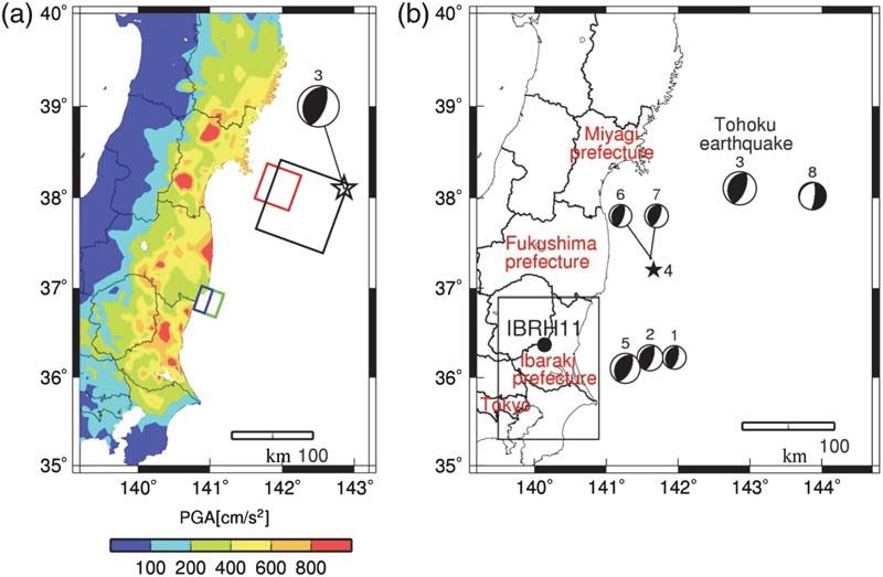
654                                       T. Satoh, T. Hayakawa, M. Oshima, H. Kawase, S. Matsushima, F. Nagashima, and K. Tobita

Figure 1. (a) The epicenter (denoted by a star; Japan Meteorological Agency [JMA]), the centroid moment tensor (CMT) solution
(National Research Institute for Earth Science and Disaster Prevention [NIED]), and the source model (Satoh, 2012) for the 2011 Tohoku
earthquake. The four rectangles indicate strong-motion generation areas (SMGAs), where strong motions in the frequency range of
0.05–10 Hz were generated (Satoh, 2012). The contours indicate the distributions of peak ground accelerations (PGAs; the geometrical
mean of two horizontal components) observed at the ground surface by 909 strong-motion stations installed by NIED, JMA, and local
governments in this area. (b) The epicenters (JMA) and the CMT solutions (NIED) for the eight earthquakes used in this study. The earthquake
without a CMT solution (EQID4 in Table 1) is indicated by a star.

     The velocity and Q (or damping) structures are impor-              strong ground shaking (e.g., Arai, 2006; Sawazaki et al.,
tant for calculating the theoretical site response. S-wave              2006; Yamada et al., 2010). We examine the time-varying
velocity (V S ) and QS are parameters that are particularly in-         nonlinear behavior using records of several time windows
fluential on horizontal ground motions. At IBRH11, P- and               during the 2011 Tohoku earthquake and aftershocks ob-
S-wave logging from the surface to a depth of 103 m, which              served at IBRH11.
had a V S of 2100 m=s, was performed by NIED. However, Q
was not explored. The observed H=HB spectral ratios of
                                                                                                       Data
weak motions usually show some differences from the theo-
retical H=HB calculated using 1D wave propagation theory                     Weak- and Strong-Motion Records
based on P- and S-wave logging results (Satoh, Kawase, and
                                                                             In Figure 1a, the epicenter estimated by JMA and the
Sato, 1995, Satoh, Sato, and Kawase, 1995). Therefore, in
                                                                        centroid moment tensor (CMT) estimated by NIED are
this study, we invert the V S and QS structures from the seis-
                                                                        shown together with the four strong-motion generation areas
mic bedrock to the surface in the linear regime using three
                                                                        (SMGAs) estimated by Satoh (2012) for the 2011 Tohoku
different methods. The first method is Rayleigh-wave inver-
                                                                        earthquake. The contours indicate the PGA distributions of
sion using array records of microtremors (e.g., Horike, 1985;           the geometrical mean of two horizontal components ob-
Matsushima and Okada, 1990; Satoh, Kawase, and Matsush-                 served at the strong-motion stations installed by NIED, JMA,
ima, 2001). The second method is S-wave inversion using the             and local governments. The PGAs at the ground surfaces of
H=HB of weak motions based on the 1D wave pro-                          909 strong-motion stations are used for the contour maps in
pagation theory (e.g., Satoh, 2006). The third method is in-            Figure 1a. Figure 1b shows the epicenters estimated by JMA
version using horizontal-to-vertical (H/V) spectral ratios of           and the CMT solutions estimated by NIED for the eight earth-
weak motions based on the diffuse-field theory for plane                quakes used in this study. Their source parameters and PGAs
waves recently proposed by Kawase et al. (2011). Inversions             at IBRH11 are listed in Table 1. The origin times are given as
based on the diffuse-field theory were done by Nagashima                Japan Standard Time. EQID3 is the mainshock of the 2011
et al. (2012) and Ducellier et al. (2013) for different stations.       Tohoku earthquake and EQID8 is the Mw 7.2 earthquake that
     Concerning soil nonlinearity, it has been shown that               occurred near the Japan trench mentioned in the Introduction
nonlinear effects remain for a certain amount of time after             section. The other earthquakes are interplate earthquakes
Site Effects on Large Ground Motions at KiK-net Iwase Station IBRH11 during the 2011 Tohoku Earthquake 655
Table 1
Earthquakes Used in This Study
Origin Time (JST)* Latitude (N)* Longitude (E)*
EQID yyyy/mm/dd hh:mm:ss.s (°) m s (°) m s Depth (km)* Mw † PGA:N–S (cm=s2 )‡ PGA:E–W (cm=s2 )‡
1 2008/05/08 01:02:00.3 141 56 55 36 13 52 60.0 6.2 25.8 27.1
2 2008/05/08 01:45:18.8 141 36 29 36 13 41 50.6 6.8 68.3 70.4
3 2011/03/11 14:46:18.1 142 51 40 38 6 13 23.7 9.0 814.9 827.0
4 2011/03/11 15:12:58.4 141 39 37 37 12 17 27.0 (6.7) 47.0 51.1
5 2011/03/11 15:15:34.5 141 15 55 36 6 30 43.2 7.8 272.7 287.7
6 2011/05/14 08:35:51.0 141 37 42 37 19 40 40.9 6.0 31.8 38.6
7 2011/11/24 04:24:30.5 141 36 47 37 19 48 45.4 6.1 37.2 37.8
8 2012/12/07 17:18:20.3 143 52 1 38 1 12 49.0 7.2 186.7 230.1
*By Japan Meteorological Agency (JMA). JST is Japan Standard Time.
†M
w is obtained using the relation between M w and seismic moment from Kanamori (1977). The seismic moment is estimated by National
Research Institute for Earth Science and Disaster Prevention (NIED) as F-net centroid moment tensor (CMT) solutions except for the mainshock
EQID3, which is estimated by JMA. The magnitude for EQID4 is the JMA magnitude (MJMA ) because the CMT solution was not determined.
‡Peak ground accelerations observed at the surface station of IBRH11.
with M w ≥ 6:0 which occurred offshore from Ibaraki and Fu- spectra observed at the surface station IBRH11 during
kushima prefectures, near IBRH11. EQID5 is the largest the Tohoku earthquake. The PGAs and PGVs were approx-
2011 Tohoku aftershock, which occurred 30 min after the imately 800 cm=s2 and 60 cm=s for two horizontal compo-
mainshock, and EQID 4 is the JMA magnitude (M JMA ) 6.7 nents, respectively. Windows A, C, B, and D are mainly
earthquake that occurred 2 min before EQID5. The PGAs of used in the equivalent-linear analysis to evaluate the time
the geometrical means of the two horizontal components of dependence of the nonlinear behavior. Windows A, C,
EQID3, 5, and 8 at IBRH11 are approximately 820, 280, and and D have durations of 20 s each, and window B has a
200 cm=s2 , respectively. The PGAs of the other earthquakes duration of 30 s to cover the main portion of the S wave.
range from approximately 30 to 70 cm=s2 . The rectangular Windows B1, B2, C1, and C2 are used to show the effects
area in Figure 1b corresponds to the area shown in Figure 2. of duration on the observed H=HB ratios by comparing their
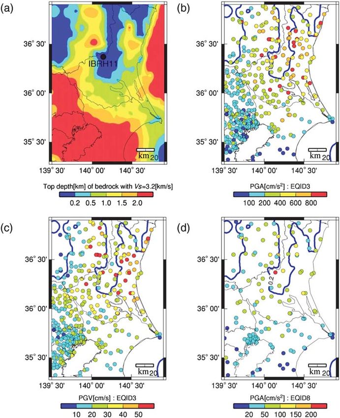
Figure 2a shows the depth of the seismic bedrock with a H=HB ratios with those of window B.
V S of 3200 m=s based on the 3D model with grid spacing of The subsurface structure models explored by NIED and
approximately 1 km created by the Headquarters for Earth- HERP and those inverted in this study are shown in Table 2.
quake Research Promotion (HERP). In this 3D model, the The PS logging and the boring survey from a depth of 106 m
engineering bedrock with a V S of 350 m=s is the topmost to the surface were done by NIED. Accelerometers were in-
layer. The depth of the seismic bedrock is shallow in the area stalled at the ground surface and a depth of 103 m by NIED.
around IBRH11, and is estimated by HERP to be approxi- The V S and QS structures inverted in this study are explained
mately 140 m underneath IBRH11. The locations of 384 in the following sections in detail. The damping factor
strong-motion stations and their PGAs and PGVs during the h 1=2QS instead of QS is shown in Table 2.
Tohoku earthquake (EQID3) are shown in Figure 2b and 2c,
respectively. Both PGAs and PGVs are large at IBRH11. The
areas with large PGVs in Ibaraki prefecture are generally the Array Records of Microtremors
areas with deep seismic bedrock. Although the seismic bed-
rock depth just beneath IBRH11 is less, the PGVs at IBRH11 We conducted the array measurement of microtremors
were large. This indicates that the shallow structure above the for 29 March 2012 at IBRH11 to estimate the shallow V S
seismic bedrock affects the large PGVs at IBRH11. Figure 2d structure. We used DATAMARK JU210, which is a portable
shows the NIED strong-motion stations during EQID8 and data logger with three-component accelerometers developed
their PGAs. The strong-motion records of the JMA and local by HAKUSAN and NIED (Senna et al., 2006). Three differ-
governments have not yet been distributed. The PGA at ent-sized arrays, a large one (L array), a medium one (M ar-
IBRH11 was very large compared to those at the other sta- ray), and a small one (S array), were deployed near the
tions in Figure 2d, and was the second largest among 961 strong-motion station IBRH11. For each array, microtremors
strong-motion stations observed by NIED, as previously were simultaneously recorded at seven observation points
mentioned. The large PGAs at IBRH11 during both Tohoku that were arranged in a cross shape. The minimum spans of
earthquake and EQID8 suggest strong-site effects on the the S, M, and L arrays were 4, 7, and 10 m, and their maxi-
high-frequency components. mum spans were 17.0, 19.7, and 36.0 m, respectively. The
Figure 3 shows the three-component accelerograms, observed duration of each array was 15 min with a sampling
the velocity waveforms calculated by numerical integration frequency of 200 Hz. Each record of the vertical component
with a low-cut filter of 0.1 Hz, and the acceleration Fourier was divided into 88 time windows of 20.48 s in length by656 T. Satoh, T. Hayakawa, M. Oshima, H. Kawase, S. Matsushima, F. Nagashima, and K. Tobita
Figure 2. (a) The depth contours of the seismic bedrock with V S of 3200 m=s based on the Headquarters for Earthquake Research
Promotion (HERP) 3D model with grid spacing of approximately 1 km in the rectangular area shown in Figure 1b. The blue lines in panels
(b), (c), and (d) indicate the contour for which the top depth of the bedrock is less than 0.2 km. (b) The locations of 384 strong-motion stations
and the PGAs during the Tohoku earthquake (EQID3). (c) As (b), but for PGVs during the Tohoku earthquake. (d) The locations of the NIED
strong-motion stations and the PGAs during EQID8.
overlapping the data in half of the length of the window. briefly described below. We first estimate a phase velocity
Some noise-contaminated windows were removed. for each time window of the microtremors by using the high-
resolution frequency–wavenumber (f-k) method of Capon
Methods (1969). Then, we omit some outlying data using a test of sig-
nificance and calculate the average and the standard devia-
Rayleigh-Wave Inversion Using Array tion of the phase velocities at each frequency. Finally, the
Records of Microtremors four V S values in the first to sixth layers shown in Table 2
The Rayleigh-wave inversion procedure using array re- are inverted using the averaged phase velocities to fit the fun-
cords of microtremors is the same method as that described damental mode of Rayleigh waves (Schwab and Knopoff,
by Satoh, Kawase, and Matsushima (2001), and will be 1970) using the quasi-Newton method (Fletcher, 1972).Site Effects on Large Ground Motions at KiK-net Iwase Station IBRH11 during the 2011 Tohoku Earthquake 657
The thickness and P-wave velocity (V P ) of each layer is fixed
using the PS logging results from NIED. The density ρ is
given by the relationship ρ 0:31V 1=4 P (Gardner et al.,
1974), in which ρ is in g=cm3 and V P is in m=s. The V P and
ρ for the other layers in the inversions using H=HB and H/V
below are calculated in the same manner.
Inversion of V S and QS Using the H=HB
of Weak Motions
We use the S-wave inversion method of Satoh (2006),
who applied the very-fast-simulated re-annealing method
(Ingber, 1989; Ingber and Rosen, 1992) to estimate V S and
QS by using the H=HB of weak motions. The parameters that
we used in the very-fast-simulated re-annealing method are
the same as those used by Satoh (2006). The V S of only the
sixth to eighth layers and the QS of the first to eighth layers in
Table 2 are inverted, assuming vertically incident S waves in
the 1D layered media. The V S from the first to fifth layers are
fixed to those inverted using microtremors. As the sensitivity
of the V S of the sixth layer inverted using microtremors was
found to be low, it was reinverted using H=HB . In the same
manner as Satoh (2006), QS is modeled as a function of fre-
quency f and V S in meters per second as
VS
Qs fa : 1
2 × 10b
We invert one common parameter b for the first to sixth
layers deposited in the Quaternary, another b for the seventh
layer, and one more b for the eighth layer to reduce the total
number of inverted parameters. The frequency-dependent
parameter a is a common parameter for all layers and is esti-
mated to be zero. In the initial model, we assume a 0:0,
b 2:0, the V S value for the sixth layer is 459 m=s estimated
from microtremors, and the V S values for the seventh and
eighth layers are based on the PS logging results.
When we represent the theoretical H=HB by M and the
observed H=HB for the jth earthquake by Oj, the objective
function Ex for an unknown vector parameter x is defined
by equation (2):
0
Pimax Mfi −Oj fi
X N
B iimin j wf i j
Ex @q
Pimax Mfi Pimax Oj fi
j1
iimin wf i iimin wf i
1
Pimax log10 Mf i −log10 Oj f i
iimin j wf i j C
Figure 3. (a) Acceleration waveforms, (b) velocity waveforms,
and (c) acceleration Fourier amplitudes observed at the ground sur-
Pimax log10 Mfi Pimax log10 Oj fi A; 2
q
iimin wf i iimin wf i
face of IBRH11 during the 2011 Tohoku earthquake. N–S, E–W,
and U–D stand for the north–south, east–west, and up–down (ver-
tical) components, respectively. The zero second time is 60 s after in which fi is the ith frequency. In this study, fimin is set at
the earthquake origin time estimated by JMA. The arrows with A, B, 0.2 Hz and fimax at 20 Hz. Here N is the number of observed
C, and D at the top of the figure indicate the time windows mainly Oj . We use two horizontal components of four earthquakes
used in the equivalent analysis. The arrows with B1, B2, C1, and C2
denote the time windows used to check the effects of duration on the
(EQID1, 2, 6, and 7), during which soil behavior is in the
difference of surface-to-borehole (H=HB ) ratios by comparing linear regime, and thus, N is eight. Records of EQID4, which
H=HB ratios for window B. The Fourier amplitudes in (c) are com- occurred approximately 27 min after the 2011 Tohoku earth-
puted using window B. quake, are not used because the nonlinear effects caused by658 T. Satoh, T. Hayakawa, M. Oshima, H. Kawase, S. Matsushima, F. Nagashima, and K. Tobita
Table 2
The Subsurface Structure at IBRH11
Damping Factor
Thickness Density V S Inverted in V S by V P by Inverted in
Number (m)* (g=cm3 )† This Study (m=s) Logging (m=s)‡ Logging (m=s)‡ This Study Nature of Soil‡
1 2.0 1.47 123 130 500 0.022 Surface soil
2 5.5 143 180 0.019 Surface soil
3 2.5 Weathering granite
4 6.0 1.93 264 240 1500 0.010 Gravel
5 4.0 Gravelly clay
6 10.0 2.07 381 450 2000 0.007 Tertiary or older period rock
7 73.0 2.57 2371 2100 4700 0.034 Tertiary or older period rock
8 141.1 0.001 Tertiary or older period rock
9 2.65 3200 5500 Tertiary or older period rock
*The eighth layer is estimated in this study. The others are surveyed by logging by National Research Institute for Earth Science and Disaster
Prevention (NIED)
†
Calculated from V P using the relation of Gardner et al. (1974).
‡
From NIED except for V S and V P of the ninth layer, which are obtained from Headquarters for Earthquake Research Promotion (HERP).
the 2011 Tohoku earthquake remain in the records of EQID4, based on the HERP 3D model. TF1 0; f is the transfer func-
as shown later. The weighting function wfi is given as tion of horizontal motion caused by vertically incident S waves.
1 TF3 0; f is the transfer function of vertical motion caused by
wfi : 3 vertically incident P waves. QS is modeled by equation (1). V P
log10 f i − log10 f i−1
is fixed to the value of the PS logging and QP is modeled as
Equations (2) and (3) are the same as those in Satoh (2006).
1 VP
The higher-mode peaks and troughs are easily contaminated QP fa ; 6
by scattering waves and other waves, which are not modeled c 2 × 10b
by 1D wave propagation theory, and so we use equation (3) to in which a and b are the same as in equation (1). Parameter a
give added weight to the lower frequencies. for the eighth layer in equations (1) and (6) is fixed to be zero,
as in the other layers. We compare the theoretical H/V ratios
Inversion for H/V Spectral Ratios Based on the for c 1, c 2, and c 3 in equation (6), because it has
Diffuse-Field Theory for Plane Waves been shown that QS is approximately one to two times as much
We estimate the thickness and QS of the eighth layer in as QP in the frequency range higher than approximately 1 Hz
Table 2 based on the diffuse-field theory for plane waves pro- for sedimentary soils (Kinoshita, 2008) and rocks (Yoshimoto
posed by Kawase et al. (2011) and using the H/V spectral et al., 1993). We found that parameter c is not sensitive to the
ratios observed at the surface. We briefly describe the con- theoretical H/V ratios. Therefore, we select c 3 because it
cept of Kawase et al. (2011). gives the smallest Ex. These assumptions are set to reduce
If many epicenters are randomly distributed, the average the trade-offs between V P and V S , and between QP and QS .
H/V ratio in diffuse fields is represented as The observed H/V spectral ratio for each earthquake
is calculated using the three components H1 , H2 , and V for
s
S-wave windows in equation (7):
Hf 2ImG1D 11 z; z; f
; 4 s
Vf ImG33 z; z; f
1D
Hf H21 f H22 f
: 7
in which G1D11 G22 is the Green’s function of the horizontal
1D
Vf V 2 f
component for a 1D structure at an observation point pro-
duced by a unit harmonic horizontal load acting at excitation We apply the very-fast-simulated re-annealing method (In-
level z, G1D
33 is the corresponding Green’s function of the ver- gber, 1989; Ingber and Rosen, 1992) to this inversion. The
tical component, and Im· is the imaginary part. When an objective function is the same as that in equation (2) except
observation point is at the ground surface, equation (4) can for Mf, which is now replaced by the average of the H/V
be written as spectral ratios for four earthquakes, and so N in equation (2)
s is equal to one.
Hf 2αH TF1 0; f
j j; 5
Vf βH TF3 0; f Inversion Results for the Subsurface Structure
in which αH and βH are V P and V S at the seismic bedrock, The phase velocities estimated from microtremors by the
respectively. We assume αH 5500 m=s and βH 3200 m=s f-k method (Capon, 1969) and the theoretical phase velocitiesSite Effects on Large Ground Motions at KiK-net Iwase Station IBRH11 during the 2011 Tohoku Earthquake 659
with the observed H/V ratios. The difference between the two
theoretical H/V ratios is small. This means that the inverted
thickness of 141 m is not well constrained. However, this re-
sult shows that the observed H/V ratios are well simulated by
the diffuse-field theory using a structure inverted by different
data such as microtremors and H=HB ratios. In other words,
this result supports the validity of the application of the dif-
fuse-field theory to the H/V ratios of weak motion.
Simulation of Weak and Strong Motions Using
Equivalent-Linear Analysis
We simulate the weak and strong motions observed at
the surface using borehole records at a depth of 103 m with
the equivalent-linear analysis method (Schnabel et al., 1972).
Equivalent-linear analysis in the frequency domain has the ad-
vantage of being able to separate incident (upgoing) and re-
flected (downgoing) waves from borehole records, unlike
time-domain nonlinear analysis. Because one of our purposes
is to estimate the incident waves (or outcrop waves) at the bed-
Figure 4. Comparison between the phase velocities estimated rock during the Tohoku earthquake to investigate site effects
from array records of microtremors and those of the theoretical cal- on large ground motions, we apply equivalent-linear analysis
culation for the fundamental mode of Rayleigh waves with the PS in this study. To examine the temporal change in the soil non-
logging (broken line) and inverted (solid line) structures. The bars linearity, we simulate the ground motions at the surface using
indicate the ranges of the average one standard deviation. equivalent-linear analysis for different time windows (A, B, C,
and D) during the 2011 Tohoku earthquake (as shown in
for the fundamental mode of Rayleigh waves (Schwab and Fig. 3) and the other earthquakes listed in Table 1.
Knopoff, 1970) with the inverted and PS logging structures The dynamic properties, that is, the strain-dependent
are shown in Figure 4. The phase velocities with the inverted shear modulus ratio G=G0 and the damping factor h as a
structure are smaller than those with the PS logging structure function of the effective shear strain, are considered for the
and agree well with the observed phase velocities. The in- first to fifth layers of Quaternary age on the basis of empirical
verted V S from the first to third layers are found to be smaller relations derived from many laboratory test results (Yasuda
than the V S from PS logging, as shown in Table 2. and Yamaguchi, 1985; Fukumoto et al., 2009). The empirical
Figure 5 shows the observed H=HB ratios and the theo- relations of Yasuda and Yamaguchi (1985) for sedimentary
retical H=HB ratios for S waves. The observed H=HB ratios soils are modeled using the soil-particle size and the effective
calculated from the weak motions of EQID1, 2, 6, and 7 are confining pressure. The average soil-particle size is esti-
shown in Figure 5a, and the average of the observed H=HB mated from the soil classifications (Yasuda and Yamaguchi,
ratios is shown in Figure 5b and c. The theoretical H=HB 1985; Towhata, 2008). The larger the size of soil particles,
ratios for the S waves in Figure 5b are computed using the the greater the effect of nonlinearity. The empirical relations
structure with the PS logging results and the structure with of Yasuda and Yamaguchi (1985) are used for the first to fifth
the V S from the first to fourth layers revised using data from layers, except for the third layer. There are no proper rela-
microtremors, assuming a damping factor of 2%. The theo- tions for the third layer, sedimentary soft rocks with
retical H=HB ratios for the S waves in Figure 5c are calcu- V S < 300 m=s. The empirical relations of Fukumoto et al.
lated using the inverted structure shown in Table 2. The (2009) are modeled using the plasticity index (PI) for
theoretical H=HB based on the PS logging results cannot sedimentary soft rocks with V S > 300 m=s. The larger the
reproduce the higher-peak frequencies. It is thus confirmed PI value, the smaller is the effect of nonlinearity. Therefore,
that the theoretical H=HB based on the structure revised only we apply the relation with PI less than 20, which is the small-
using data from microtremors is better than that based on PS est PI used in the empirical relations of Fukumoto et al.
logging results, but is worse than the inverted structure. (2009), to the third layer.
Figure 6 shows the observed and theoretical H/V ratios Figure 7 shows the observed H=HB ratios for windows
with the inverted structure. The observed H/V ratios calcu- B1, B2, B, C1, and C2 with different durations shown in
lated from the weak motions of EQID1, 2, 6, and 7 are shown Figure 3. The differences among them are small because
in Figure 6a and the average of these observed H/V ratios is large motions of the main portions of the S wave with short
shown in Figure 6b. Two theoretical H/V ratios with the durations control the H=HB ratios. The simulated and ob-
thickness of the eighth layer being 0 and 141 m are compared served H=HB ratios for window B during the 2011 Tohoku
in Figure 6b. The theoretical H/V ratios agree reasonably well earthquake are shown in Figure 8. The simulated H=HB660 T. Satoh, T. Hayakawa, M. Oshima, H. Kawase, S. Matsushima, F. Nagashima, and K. Tobita
Figure 6. (a) H/V ratios of weak motions observed during
EQID1, 2, 6, and 7. (b) Comparison between the average of the
observed H/V ratios and the H/V ratios computed on the basis
of the diffuse-field theory for plane waves with the inverted struc-
ture. The H/V ratios are calculated for two cases with the thickness
of the eighth layer being 0 m and an inverted value of 141 m.
ratios can reasonably represent the observed H=HB ratios. By
comparing Figure 8 with Figure 6, we find that both peak fre-
quencies and amplitudes of the H=HB ratios for window B
are noticeably smaller than those of the weak motions.
The simulated and observed acceleration waveforms at
the surface for both north–south (N–S) and east–west (E–W)
components for window B are shown in Figure 9. We find that
the equivalent-linear analysis (second row) works well, but
the linear analysis (third row) significantly overestimates the
Figure 5. (a) H=HB ratios of weak motions observed during records observed at the surface (first row). The PGA values of
EQID1, 2, 6, and 7. (b) Comparison between the average of the the waves simulated by the linear analysis are approximately
observed H=HB ratios and the H=HB ratios computed on the basis twice the observed values. However, the waves simulated by
of the 1D wave propagation theory for S waves with a structure
based on PS logging and a structure revised only using data from the equivalent-linear analysis are slightly richer in high-fre-
microtremors, assuming a damping factor of 2%. (c) Comparison quency components because the simulated H=HB slightly
between the average of the observed H=HB ratios and the H=HB overpredicts high frequencies and underpredicts low frequen-
ratios computed on the basis of the 1D wave propagation theory cies, as shown in Figure 8. We will consider the misfit between
for S waves with the inverted structure given in Table 2.
the observed and simulated results in the Discussion section.Site Effects on Large Ground Motions at KiK-net Iwase Station IBRH11 during the 2011 Tohoku Earthquake 661
Figure 7. Observed H=HB ratios of the N–S components for
windows B, B1, B2, C1, and C2 during the 2011 Tohoku earthquake.
The depth profiles for G=G0, h, and the effective shear-
strain γ eff from the equivalent-linear analysis are shown in
Figure 10. Here, γ eff is 0.65 times the maximum shear strain
and is used as the shear strain to obtain G=G0 and h. The
layers subject to nonlinearity are divided into thin layers with
thicknesses of approximately 2 m for application of the
equivalent-linear analysis. The stiffness G is represented
by G ρV 2S. Therefore, the smallest G=G0 0:25 in this
figure gives a V S reduction of 50%. The maximum γ eff of
the N–S component reaches 5 × 10⁻³ , but the equivalent-lin-
ear analysis works reasonably well. The γ eff of the granite at
depths between 20 and 30 m in Table 2 is small, that is, on
the order of 2 × 10⁻⁵ . Therefore, the effects of nonlinearity
of the granite would be negligible even if strain-dependent
G=G0 and h are considered.
The G=G0 and h curves used in the equivalent-linear
analysis and the resulting G=G0 and h for each layer from Figure 8. Comparison between the H=HB ratios computed us-
ing equivalent-linear analysis and the observed H=HB ratios of
the surface to a depth of 20 m are shown in Figure 11. The (a) the N–S and (b) the E–W components for window B during
G=G0 and h curves are assumed on the basis of empirical the 2011 Tohoku earthquake.
relations derived from many laboratory test results (Yasuda
and Yamaguchi, 1985; Fukumoto et al., 2009), as mentioned Figure 13. These are the spectral ratios of the waves at
previously. Laboratory test results for weathering granite are the surface to the hypothetical outcrop waves. The two am-
rare, and hence we took the G=G0 and h curves of the third plification factors in the linear regime are almost the same
layer with V S 143 m=s in Table 2 as the empirical relation because the large amplifications are mainly controlled by
for rock with V S > 300 m=s of Fukumoto et al. (2009). To the strong impedance contrast between the soft layers with
show the sensitivity of the G=G0 and h curves, we alter the V S ≤ 381 m=s and the layer with V S 2371 m=s at a depth
G=G0 and h curves of the third layer to be the same as those of 30 m. The impedance contrast is larger than that based on
of the first and second layers. The differences between the PS logging results shown in Table 2. We also confirm
the G=G0 and h curves are relatively large, as shown in that the amplification factor for GL0m/GL-103m by using
Figure 11. Figure 12 shows the simulated H=HB ratios with the equivalent-linear analysis for the N–S component is
the original and replaced G=G0 and h curves, together with much smaller than that from the linear analysis. The ampli-
observed H=HB of the N–S components for window B. It is fication factor for GL0m/GL-103m shows a peak amplitude
confirmed that the effects of the assumed G=G0 and h curves of 15 at the first predominant frequency of 2.5 Hz from the
of the third layer are not very large. linear analysis. The first predominant frequency is reduced to
The theoretical amplification factors for S waves going approximately 1.7 Hz, and the peak amplitude is reduced to 6
to the surface from two different layers are compared in because of the soil nonlinearity. These results mean that the662 T. Satoh, T. Hayakawa, M. Oshima, H. Kawase, S. Matsushima, F. Nagashima, and K. Tobita
Figure 9. Computed and observed acceleration waveforms of (a) the N–S and (b) E–W components for window B at the surface. The first
traces show the observed waves. The second and third traces show the waves calculated using the equivalent-linear and linear analyses,
respectively.
Figure 10. The depth profiles of the shear modulus ratio G=G0 ,
the damping factor h, and the effective shear strain γ eff estimated
using equivalent-linear analysis for window B.
Figure 11. The shear modulus ratio G=G0 , the damping factor
h used for the equivalent-linear analysis simulation, and the result-
nonlinearity of the surface soils reduced the amplification ing G=G0 and h for each layer. The empirical relations for sedimen-
factors approximately by half compared with those in the lin- tary soils by Yasuda and Yamaguchi (1985) are used for the first to
fifth layers, except for the third layer in Table 2. The empirical re-
ear regime. lations for sedimentary soft rock from Fukumoto et al. (2009) are
Figure 14 shows the observed and simulated H=HB ra- used for the third layer.
tios of the N–S components for windows A, C, and D. The
H=HB ratio for window A simulated using equivalent-linear proximately two months after the Tohoku earthquake. The
analysis agrees well with the observed ratio. On the other effects of nonlinearity from the Tohoku earthquake would
hand, the H=HB ratios for windows C and D simulated using cause remarkable overprediction for EQID5 by using equiv-
equivalent-linear analysis are overestimated compared to the alent-linear analysis. Quantitative evaluations of the effects
observed ratios. Figure 15 shows the observed and simulated of nonlinearity due to the mainshock on the ground motions
H=HB ratios of the N–S components of the S-wave windows of EQID4 and EQID5 will be conducted in the Discussion
of EQID4, 5, and 8 using equivalent-linear analysis. The section. Similar time-varying soil nonlinearity after strong
equivalent-linear analysis for EQID4, which occurred 27 min shaking during other earthquakes has been shown by several
after the Tohoku earthquake, slightly overpredicts the H=HB researchers (e.g., Arai, 2006; Sawazaki et al., 2006; Yamada
ratio. On the other hand, the observed H=HB values of et al., 2010), although the recovery time to become linear
EQID1, 2, 6, and 7 are almost the same as those shown in again is different from site to site. The differences in recovery
Figure 6a and are well explained by the linear analysis. These times may be caused by differences in the strain levels ex-
results suggest that the effects of nonlinearity caused by the perienced and the natures of the soils.
large input in window B remained for at least 27 min after We also found that the equivalent-linear analysis
window B, but had faded before EQID6, which occurred ap- also worked well for the strong motions with PGAs ofSite Effects on Large Ground Motions at KiK-net Iwase Station IBRH11 during the 2011 Tohoku Earthquake 663
Figure 12. Comparison between the H=HB ratios computed us-
Figure 13. The theoretical 1D amplification factors for S waves
going to the surface from different layers at IBRH11. The ampli-
ing equivalent-linear analysis with original and replaced G=G0 and
fication factors are the spectral ratios between waves at the surface
h curves for the third layer and the observed H=HB ratios of the N–S
and those computed as outcrop motions at depths of either 30 or
components for window B during the 2011 Tohoku earthquake. The
103 m. The GL0m/GL-30m from the equivalent-linear analysis is
bold dashed line is added to Figure 8a.
the amplification factor of the N–S component for window B. The
other two amplification factors are calculated using linear analysis.
approximately 200 cm=s2 during EQID8, which occurred
after the recovery of the soil properties. The effective strains motions. N has a value of one because the N–S and E–W
of the layers between the surface and a depth of 20 m are on the components are independently treated. In this method, the
order of 1 × 10⁻⁴ to 4 × 10⁻⁴ . The observed and computed changes in V S and the damping factors caused by soil
H=HB values for EQID8 are different from those for the nonlinearity are directly estimated (e.g., Satoh, Sato, and
weak motions shown in Figure 6; however, their differences Kawase, 1995; Satoh, Fushimi, and Tatsumi, 2001).
are not very large. The effects of nonlinearity were small The V S values and damping factors computed using
because of the much lower level of shaking than that during equivalent-linear analysis and inverted here are shown in
the 2011 Tohoku earthquake, and hence, the strong imped- Figure 16. The V S values estimated using the two methods
ance contrast mainly contributed to the largest JMA instru- agree with each other for the E–W components, except for
mental intensity and the second largest PGA values among the top layer, but less so for the N–S components. The damp-
961 K-NET and KiK-net stations during EQID8. ing factors estimated using the two methods are different for
both N–S and the E–W components. Because six parameters
Discussion are inverted using one H=HB , there might be some trade-offs
between the parameters. Figure 17 shows the comparison
We simulated the ground motions during the 2011 between the observed and inverted H=HB ratios. The inverted
Tohoku earthquake and estimated the bedrock motions using H=HB ratios agree with the observed H=HB slightly better
equivalent-linear analysis. The equivalent-linear analysis is than with the H=HB computed using equivalent-linear
useful for strong-motion prediction as well as simulation. analysis, as shown in Figure 8. In Figure 18, we show the
However, there were slight differences between the observed acceleration waveforms at the surface computed using
and computed H=HB ratios and waveforms, as shown in equivalent-linear analysis and the inverted structures. In
Figures 8 and 9. To more precisely estimate bedrock mo- Figure 19, we show the bedrock acceleration waveforms
tions, the V S structure is inverted using H=HB ratios for win- computed by equivalent-linear analysis using the inverted
dow B. The method is the same as the inversion method structures. The bedrock motions are twice those of the inci-
using H=HB for weak motions except for the inverted param- dent (upgoing) waves at a depth of 103 m. We confirm that
eters, the searching range, and N, which is the number of the differences in the motions estimated using the two meth-
observed H=HB used for the inversion, in equation (2). The ods are small, although the V S and damping factors shown in
inverted parameters are three V S values and three damping Figure 16 show some differences.
factors from the surface to a depth of 20 m, where nonlinear- Nagashima et al. (2012) predicted the bedrock motions
ity is considered in the equivalent-linear analysis. The maxi- at K-NET MYG004 (Tsukidate) in Miyagi prefecture from
mum V S values of the searching range are assumed to be 123, records with PGAs of 1300 and 960 cm=s2 at the surface dur-
143, and 264 m=s (Table 2) estimated from the weak ing the first wave packet mainly generated from SMGA 1 of664 T. Satoh, T. Hayakawa, M. Oshima, H. Kawase, S. Matsushima, F. Nagashima, and K. Tobita
Figure 15. Comparison between the H=HB ratios computed us-
Figure 14. Comparison between the H=HB ratios computed us- ing equivalent-linear analysis and the observed H=HB ratios of the
ing equivalent-linear analysis and the observed H=HB ratios of the N–S components for EQID4, 5, and 8. EQID4 and 5 occurred ap-
N–S components for windows A, C, and D during the 2011 Tohoku proximately 30 min after the 2011 Tohoku earthquake and EQID8
earthquake. occurred on 7 December 2012.Site Effects on Large Ground Motions at KiK-net Iwase Station IBRH11 during the 2011 Tohoku Earthquake 665
Figure 16. The depth profiles for V S and the damping factor h
computed using equivalent-linear analysis and inverted using the
H=HB ratios for window B.
Figure 1a. The PGAs of the estimated bedrock motions were
450 and 350 cm=s2 , both of which are similar to those esti-
mated at IBRH11 in this study. Satoh (2012) showed using Figure 17. Comparison between the H=HB ratios computed us-
the empirical Green’s function method that the main part cor- ing the inverted structures and the observed H=HB ratios of (a) the
N–S and (b) the E–W components for window B.
responding to window B at a station in the northern part of
Ibaraki prefecture was composed of three wave packets gen-
comparison with those inverted using the weak motions of
erated from SMGAs 2, 3, and 4, all of which reached the
EQID1, 2, 6, and 7. This result means that the effects of non-
station almost simultaneously. Considering the rupture linearity caused by the mainshock lasted until events EQID4
starting time of the SMGAs and the travel time from them, and EQID5. Therefore, we perform the equivalent-linear
window B at IBRH11 is also composed of three fully over- analysis for EQID5 using V S and damping factors inverted
lapping wave packets. This source effect must have contrib- using the H=HB ratios for EQID4. The simulated and ob-
uted to the large bedrock motion at IBRH11. served H=HB ratios of the N–S components for EQID5 are
Finally, we estimate the V S and the damping factors of shown in Figure 22. The agreement between the simulated
the first to third layers using the H=HB ratios for EQID4 and and observed H=HB ratios in Figure 22 is better than that
the same inversion method. The inverted and observed H=HB in Figure 15b. This result shows that the effects of the non-
ratios of the N–S components for EQID4 are shown in linearity caused by strong shaking during the Tohoku earth-
Figure 20. The inverted H=HB ratios agree with the observed quake remained for at least approximately 30 min, thereby
H=HB better than the H=HB computed by the equivalent- causing remarkable overprediction for EQID5 in Figure 15b.
linear analysis shown in Figure 15a. The V S and damping
factors inverted using the weak motions of EQID1, 2, 6, and
Conclusions
7, the weak motions of EQID4 (N–S components), and the
strong motions of EQID3 (N–S components) are compared During the 2011 Mw 9.0 Tohoku earthquake, large
in Figure 21. The reduction in V S and the increase in the ground motions with horizontal components having PGAs of
damping factor of the first layer for EQID4 are found by more than 800 cm=s2 and PGVs of nearly 60 cm=s were666 T. Satoh, T. Hayakawa, M. Oshima, H. Kawase, S. Matsushima, F. Nagashima, and K. Tobita
Figure 18. The acceleration waveforms at the surface of (a) the N–S and (b) the E–W components computed using equivalent-linear
analysis (upper panel) and the inverted structures for window B (lower panel).
Figure 19. Bedrock acceleration waveforms of (a) the N–S and (b) the E–W components calculated using equivalent-linear analysis
(upper panel) and using the inverted structures for window B (lower panel). The bedrock motions are twice those of the incident (upgoing)
waves at a depth of 103 m.
observed at one of the KiK-net stations, Iwase (IBRH11), frequency was reduced to approximately 1.7 Hz. These re-
Japan. IBRH11 was one of the stations with quite large sults show that the nonlinearity of the surface soils reduced
ground motions out of at least 2174 stations observed by the amplification factors of the ground motion by half com-
public organizations in Japan. In this study, we investigated pared with those in the linear regime. The PGAs of bedrock
the causes of the large ground motions by inverting the sub- motions at a depth of 103 m with V S 2371 m=s estimated by
surface structures and simulating the ground motions using equivalent-linear analysis reached approximately 500 cm=s2,
linear and equivalent-linear analyses. The V S and QS struc- which is approximately twice that of the borehole PGAs.
tures from the seismic bedrock to the surface in the linear re- The soil nonlinearity generated by the strong ground
gime were inverted from the phase velocities of microtremor shaking due to the 2011 Tohoku earthquake remained for
array measurements using the Rayleigh-wave inversion, the at least approximately 30 min and became linear again within
H=HB spectral ratios of weak motions using S-wave inversion two months. The equivalent-linear analysis also worked well
based on 1D wave propagation theory, and the H/V spectral for simulations of strong motions with PGAs of approxi-
ratios of weak motions using the inversion based on the dif- mately 200 cm=s2 during the 7 December 2012 M w 7.2
fuse-field theory for plane waves (Kawase et al., 2011). earthquake. As the effects of nonlinearity were not as large,
Using the inverted structure, the main cause of the large because much less shaking occurred than had happened
ground motions was found to be the strong impedance con- during the 2011 Tohoku earthquake, the strong impedance
trast between soft layers with V S ≤ 381 m=s and a layer with contrast mainly contributed to the largest JMA instrumental
V S 2371 m=s at a depth of 30 m. The PGA of the N–S intensity scale and the second largest PGAs among 961
component at the surface during the 2011 Tohoku earthquake strong-motion stations during this M w 7.2 earthquake.
simulated by linear analysis using borehole records for a
depth of 103 m was more than 2000 cm=s2 , which was ap-
Data and Resources
proximately twice as large as the observed values. On the
other hand, the ground motions simulated by the equiva- The strong-motion records observed at K-NET and KiK-
lent-linear analysis were in reasonable agreement with those net stations were obtained from the National Institute for
observed. The amplification factor for S waves between the Earth Science and Disaster Prevention (NIED) at http://
surface and a depth of 30 m was estimated using linear analy- www.kyoshin.bosai.go.jp/kyoshin/ (last accessed December
sis to be a factor of 15 at the first predominant frequency of 2012). The strong-motion records observed at the Japan
2.5 Hz. Here these computed amplification factors are the Meteorological Agency (JMA) and local governments (Ao-
spectral ratios of the motions at the surface to the hypotheti- mori, Iwate, Miyagi, Akita, Yamagata, Fukushima, Ibaraki,
cal outcrop motions. Because of the soil nonlinearity, the Tochigi, Gunma, Saitama, Kanagawa, Niigata, Yamanashi,
peak amplitude was reduced by a factor of 6 and the peak Nagano, Shizuoka, Wakayama, Kumamoto prefectures, Tokyo,Site Effects on Large Ground Motions at KiK-net Iwase Station IBRH11 during the 2011 Tohoku Earthquake 667
Figure 20. Comparison between the H=HB ratios computed us-
ing the inverted structure and the observed H=HB ratios of the N–S Figure 22. Comparison between the H=HB ratios computed us-
components for EQID4. ing equivalent-linear analysis with the structure inverted using the
H=HB ratios for EQID4 and the observed H=HB ratios of the N–S
components for EQID5.
accessed December 2012). The PS logging and boring survey
results at IBRH11 were obtained from http://www.kyoshin.
bosai.go.jp/kyoshin/pubdata/kik/sitejpeg/IBRH11-J.jpeg and
http://www.kyoshin.bosai.go.jp/cgi-bin/kyoshin/db/sitedat.
cgi?0+IBRH11+kik, respectively (last accessed December
2012). The 3D structure model was provided by the Head-
quarters for Earthquake Research Promotion (HERP) at
http://www.jishin.go.jp/main/chousa/09_choshuki/dat/index.
htm (last accessed December 2012). Hypocentral information
up through May 2011 was obtained from the CD-ROM. The
Seismological and Volcanological Bulletin of Japan May,
2011 by JMA and after that date from the JMA Unified Hypo-
center Catalog at http://www.hinet.bosai.go.jp/REGS/JMA/
jmalist.php?LANG=en (last accessed December 2012). Dig-
ital data of prefectural boundaries are obtained from National
Land Numerical Information download service at http://
nlftp.mlit.go.jp/ksj-e/index.html (last accessed December
2012) by National and Regional Policy Bureau, Ministry of
Land Infrastructure, Transport and Tourism.
Acknowledgments
This research is a collaborative research of France and Japan and
funded by Japan conducted as a part of the J-RAPID program “Quantitative
assessment of nonlinear soil response during the great Tohoku earthquake”
(P. I. Kawase) funded by Japan Science Technology Agency. We would like
Figure 21. The depth profiles of the V S and damping factor h to thank Hideo Aochi for his valuable comments on this manuscript and the
inverted using the H=HB ratios for the weak motions of EQID1, 2, 6, cooperation to microtremor measurements. We thank Robert Graves, an
and 7, the weak motions of EQID4 (N–S components), and the anonymous reviewer, and Associate Editor Ivan G. Wong for their helpful
strong motions (window B) of EQID3 (N–S components). comments. Some figures are plotted with Generic Mapping Tools (GMT;
Wessel and Smith, 1998).
and Chiba city) were obtained from a DVD-ROM, JMA-95
type accelerograms, 2011, by JMA. The centroid moment tensor References
(CMT) information determined by F-net was obtained from Arai, H. (2006). Detection of subsurface V S recovery process using micro-
NIED at http://www.fnet.bosai.go.jp/top.php?LANG=ja (last tremor and weak ground motion records in Ojiya, Japan, in Proc. of the668 T. Satoh, T. Hayakawa, M. Oshima, H. Kawase, S. Matsushima, F. Nagashima, and K. Tobita
3rd International Conference on Urban Earthquake Engineering, Satoh, T., H. Kawase, and S. Matsushima (2001). Estimation of S-wave
Tokyo Institute of Technology, Tokyo, 6–7 March 2006, 631–638. velocity structures in and around the Sendai basin, Japan using array
Bonilla, F., K. Tsuda, N. Pulido, J. Regnier, and A. Laurendeau (2011). Pre- records of microtremors, Bull. Seismol. Soc. Am. 91, 206–218.
liminary analysis of site response of K-NET and KiK-net records from the Satoh, T., H. Kawase, and T. Sato (1995). Evaluation of local site effects and
M w 9 Tohoku earthquake, special issue: First results of the 2011 off the their removal from borehole records observed in the Sendai region,
Pacific coast of Tohoku earthquake, Earth Planets Space 63, 785–789. Japan, Bull. Seismol. Soc. Am. 85, 1770–1789.
Capon, J. (1969). High-resolution frequency–wave-number spectrum Satoh, T., T. Sato, and H. Kawase (1995). Nonlinear behavior of soil sedi-
analysis, Proc. IEEE 57, 1408–1418. ments identified by using borehole records observed at the Ashigara
De Martin, F., H. Kawase, S. Matsushima, and F. Bonilla (2012). Inversion Valley, Japan, Bull. Seismol. Soc. Am. 85, 1821–1834.
of equivalent linear soil parameters during the 2011 Tohoku Earth- Sawazaki, K., H. Sato, H. Nakahara, and T. Nishimura (2006). Temporal
quake, Japan, in Proc. of the 15th World Conference of Earthquake change in site response caused by earthquake strong motion as re-
Engineering, Lisbon, Portugal, 14–28 September 2012, Paper Number vealed from coda spectral ratio measurement, Geophys. Res. Lett.
WCEE2012_2124. 33, L21303, doi: 10.1029/2006GL027938.
Ducellier, A., H. Kawase, and S. Matsushima (2013). Validation of a new Schnabel, P. B., J. Lysmer, and H. B. Seed (1972). SHAKE—A computer
velocity structure inversion method based on horizontal-to-vertical program for earthquake response analysis of horizontally layered sites,
(H/V) spectral ratios of earthquake motions in the Tohoku area, Japan, Report EERC 72-12, University of California, Berkeley.
Bull. Seismol. Soc. Am. 103, 958–970. Schwab, F., and L. Knopoff (1970). Surface-wave dispersion computations,
Fletcher, R. (1972). FORTRAN subroutines for minimization by quasi- Bull. Seismol. Soc. Am. 60, 321–344.
Newton methods, Report R7125 AERE, Harwell, England. Senna, S., S. Adachi, H. Ando, T. Araki, K. Iisawa, and H. Fujiwara (2006).
Fukumoto, S., N. Yoshida, and M. Sahara (2009). Dynamic deformation Development of microtremor survey observation system, in Proc. of
characteristics of sedimentary soft rock, J. Japan Assoc. Earthq. the 115th Society of Exploration Geophysicists of Japan Conference,
Eng. 9, no. 1, 46–61 (in Japanese with English abstract). 128–133 (in Japanese with English abstract).
Gardner, G. H. F., L. W. Gardner, and A. R. Gregory (1974). Formation Towhata, I. (2008). Geotechnical Earthquake Engineering, Springer Series in
velocity and density—The diagnostic basics for stratigraphic traps, Geomechanics and Geoengineering, Springer-Verlag, Berlin, Heidel-
Geophysics 29, 770–780. berg, 684 pp., doi: 10.1007/978-3-540-35783-4.
Hayakawa, T., T. Satoh, M. Oshima, H. Kawase, S. Matsushima, Baoyintu, Wessel, P., and W. H. F. Smith (1998). New, improved version of Generic
F. Nagashima, and K. Nakano (2012). Estimation of the nonlinearity Mapping Tools released, Eos Trans. AGU 79, 579.
of the surface soil at Tsukidate during the 2011 off the Pacific coast Yamada, M., J. Mori, and S. Ohmi (2010). Temporal changes of subsurface
of Tohoku earthquake, in Proc. of the 15th World Conference of velocities during strong shaking as seen from seismic interferometry, J.
Earthquake Engineering, Lisbon, Portugal, 14–28 September 2012, Geophys. Res. 115, B03302, doi: 10.1029/2009JB006567.
Paper Number WCEE2012_3974. Yasuda, S., and I. Yamaguchi (1985). Dynamic soil properties of undis-
Horike, M. (1985). Inversion of phase velocity of long-period microtremors turbed samples, in Proc. of the 20th Annual Convention of Japanese
to the S-wave-velocity structure down to the basement in urbanized Society of Soil Mechanics and Foundation Engineering, Nagoya,
areas, J. Phys. Earth 33, 59–96. Japan, 10–13 June 1985, 539–542 (in Japanese).
Ingber, L. (1989). Very fast simulated reannealing, Math. Comput. Model. 2, Yoshimoto, K., H. Sato, S. Kinoshita, and M. Ohtake (1993). High-frequency site
967–973. effect of hard rocks at Ashio, central Japan, J. Phys. Earth 41, 327–335.
Ingber, L., and B. E. Rosen (1992). Genetic algorithms and very fast simu-
lated reannealing: A comparison, Math. Comput. Model. 16, 87–100.
Kanamori, H. (1977). The energy release of great earthquakes, J. Geophys. Institute of Technology
Res. 82, 2981–2987. Shimizu Corporation
Kawase, H., F. J. Sánchez-Sesma, and S. Matsushima (2011). The optimal 4-17 Etchujima 3-chome, Koto-ku
use of horizontal-to-vertical (H/V) spectral ratios of earthquake mo- Tokyo 135-8530, Japan
tions for velocity structure inversions based on diffuse field theory for (T.S., T.H., M.O.)
plane waves, Bull. Seismol. Soc. Am. 101, 2001–2014.
Kinoshita, S. (2008). Deep-borehole-measured QP and QS attenuation for
two Kanto sediment layer sites, Bull. Seismol. Soc. Am. 98, 463–468. Disaster Prevention Research Institute
Matsushima, T., and H. Okada (1990). Determination of deep geological Kyoto University
structures under urban areas using long-period microtremors, Geo- Gokasho, Uji
phys. Explor. (Butsuri-Tansa) 43, 21–33. Kyoto 611-0011, Japan
Nagashima, F., H. Kawase, S. Matsushima, F. J. Sánchez-Sesma, T. (H.K., S.M.)
Hayakawa, T. Satoh, and M. Oshima (2012). Application of the H/V
spectral ratios for earthquake ground motions and microtremors at K-
NET sites in Tohoku region, Japan to delineate soil nonlinearity, in Proc. Graduate School of Engineering
of the 15th World Conference of Earthquake Engineering, Lisbon, Por- Kyoto University
tugal, 14–28 September 2012, Paper Number WCEE2012_2190. Kyoto daigaku-katsura, Nishikyo-ku
Satoh, T. (2006). Inversion of QS of deep sediments from surface-to- Kyoto 615-8530, Japan
borehole spectral ratios considering obliquely incident SH and (F.N.)
SV-waves, Bull. Seismol. Soc. Am. 96, 943–956.
Satoh, T. (2012). Inversion of source model of the 2011 off the Pacific coast
of Tohoku earthquake using empirical Green’s function method, in Kansai Electric Power Company
Proc. of the 15th World Conference of Earthquake Engineering, 6-16, Nakanoshima 3-chome, Kita-ku, Osaka-shi
Lisbon, Portugal, 14–28 September 2012, Paper Number Osaka 530-0005, Japan
WCEE2012_0974. (K.T.)
Satoh, T., M. Fushimi, and Y. Tatsumi (2001). Inversion of strain-dependent
nonlinear characteristics of soils using weak and strong motions ob- Manuscript received 24 April 2013;
served by borehole sites in Japan, Bull. Seismol. Soc. Am. 91, 365–380. Published Online 25 March 2014You can also read