Back-testing of Expected Shortfall: Main challenges and methodologies - Chappuis Halder
←
→
Page content transcription
If your browser does not render page correctly, please read the page content below

© CHAPPUIS HALDER & CO

        Back-testing of Expected
      Shortfall: Main challenges and
              methodologies

      By Leonard BRIE with Benoit GENEST and Matthieu ARSAC

                                       Global Research & Analytics1

1
  This work was supported by the Global Research & Analytics Dept. of Chappuis Halder & Co.
Many collaborators from Chappuis Halder & Co. have been involved in the writing and the reflection around this paper; hence we would like
to send out special thanks to Claire Poinsignon, Mahdi Kallel, Mikaël Benizri and Julien Desnoyers-Chehade
© Global Research & Analytics Dept.| 2018 | All rights reserved

Executive Summary
In a context of an ever-changing regulatory environment over the last years, Banks have
witnessed the draft and publication of several regulatory guidelines and requirements in order
to frame and structure their internal Risk Management.
Among these guidelines, one has been specifically designed for the risk measurement of market
activities. In January 2016, the Basel Committee on Banking Supervision (BCBS) published
the Fundamental Review of the Trading Book (FRTB). Amid the multiple evolutions discussed
in this paper, the BCBS presents the technical context in which the potential loss estimation has
changed from a Value-at-Risk (VaR) computation to an Expected Shortfall (ES) evaluation.
The many advantages of an ES measure are not to be demonstrated, however this measure is
also known for its major drawback: its difficulty to be back-tested. Therefore, after recalling
the context around the VaR and ES models, this white paper will review ES back-testing
findings and insights along many methodologies; these have either been drawn from the latest
publications or have been developed by the Global Research & Analytics (GRA) team of
Chappuis Halder & Co.
As a conclusion, it has been observed that the existing methods rely on strong assumptions and
that they may lead to inconsistent results. The developed methodologies proposed in this paper
also show that even though the ES97.5% metric is close to a VaR99,9% metric, it is not as easily
back-tested as a VaR metric; this is mostly due to the non-elicitability of the ES measure.

Keywords: Value-at-Risk, Expected Shortfall, Back-testing, Basel III, FRTB, Risk
Management
EL Classification: C02, C63, G01, G21, G17

                                               2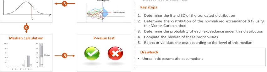
© Global Research & Analytics Dept.| 2018 | All rights reserved

Table of Contents
Table of Contents ....................................................................................................................... 3
1.     Introduction ........................................................................................................................ 4
2.     Context ............................................................................................................................... 4
     2.1.    Value-at-Risk ............................................................................................................... 5
       2.1.1.       VaR Definition ..................................................................................................... 5
       2.1.2.       Risk Measure Regulation ..................................................................................... 6
       2.1.3.       VaR Calculation ................................................................................................... 6
       2.1.4.       VaR Back-Testing ................................................................................................ 7
     2.2.    Expected Shortfall ....................................................................................................... 9
       2.2.1.       ES Definition ........................................................................................................ 9
       2.2.2.       ES Regulatory framework .................................................................................. 10
       2.2.3.       ES Calculation .................................................................................................... 10
       2.2.4.       VaR vs. ES ......................................................................................................... 11
       2.2.5.       ES Back-Testing ................................................................................................. 12
3.     ES Back-Testing ............................................................................................................... 14
     3.1.    Existing Methods ....................................................................................................... 14
       3.1.1.       Wong’s Saddle point technique.......................................................................... 14
       3.1.2.       Righi and Ceretta ................................................................................................ 17
       3.1.3.       Emmer, Kratz and Tasche .................................................................................. 22
       3.1.4.       Summary of the three methods........................................................................... 23
     3.2.    Alternative Methods .................................................................................................. 25
       3.2.1.       ES Benchmarking ............................................................................................... 25
       3.2.2.       Bootstrap ............................................................................................................ 26
       3.2.3.       Quantile Approaches .......................................................................................... 27
4.     Applications of the ES methodology and back-testing .................................................... 31
     4.1.    ES simulations ........................................................................................................... 31
     4.2.    Back-test of the ES using our alternative methods .................................................... 34
5.     Conclusion ........................................................................................................................ 41

                                                                      3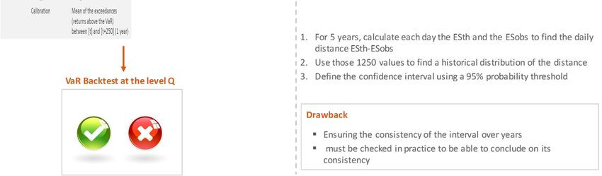
© Global Research & Analytics Dept.| 2018 | All rights reserved

1. Introduction
Following recent financial crises and their disastrous impacts on the industry, regulators are
proposing tighter monitoring on banks so that they can survive in extreme market conditions.
More recently, the Basel Committee on Banking Supervision (BCBS) announced a change in
the Market Risk measure used for Capital requirements in its Fundamental Review of the
Trading Book (FRTB), moving from the Value-at-Risk (VaR) to the Expected Shortfall (ES).
However, if the ES captures risks more efficiently than the VaR, it also has one main downside
which is its difficulty to be back-tested. This leads to a situation where banks use the ES to
perform Capital calculations and then perform the back-testing on a VaR. The focus for banks’
research is now to try to find ways to back-test using the ES, as it can be expected that regulators
will require so in a near-future.
This paper aims at presenting the latest developments in the field of ES back-testing
methodologies and introducing new methodologies developed by the Global Research &
Analytics (GRA) team of Chappuis Halder & Co.
First, a presentation of the context in which the back-testing of Expected Shortfall takes place
will be provided. This context starts with calculation and back-testing methodologies of the
Value-at-Risk, followed by a focus on the ES, analysing its calculation and how it defers from
the previous risk measure. The main issues of ES back-testing will then be exposed and
discussed.
Second, back-testing methodologies for ES will be reviewed in detail, beginning with
methodologies that have already been presented in previous years and then with alternative ones
introduced by the research department of Chappuis Halder &Co.
Third, some of the alternative back-testing methodology will be simulated on a hypothetical
portfolio and a comparison of the methodologies will be conducted.

2. Context
Recall that in January 2016, the Basel Committee on Banking Supervision (BCBS) issued its
final guidelines on the Fundamental Review of the Trading Book (FRTB). The purpose of the
FRTB is to cover shortcomings that both regulations and internal risk processes failed to capture
during the 2008 crisis. It shows a strategic reversal and the acceptance of regulators for:
   -   a convergence between risk measurement methods;
   -   an integrated assessment of risk types (from a silo risk assessment to a more
       comprehensive risk identification);
   -   an alignment between prudential and accounting rules.
One of the main requirements and evolutions of the FRTB is the switch from a Value-at-Risk
(VaR) to an Expected Shortfall risk measurement approach. Hence, Banks now face the paradox
of using the ES for the computation of their Market Risk Capital requirements and the Value-
at-Risk for the back-testing. This situation is mainly due to the difficulty of finding an ES back-
testing methodology that is both mathematically consistent and practically implementable.
However, it can be expected that upcoming regulations will require banks to back-test the ES.
                                                 4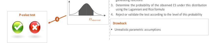
© Global Research & Analytics Dept.| 2018 | All rights reserved

The following sections aim at reminding the existing Market Risk framework for back-testing,
as most of the presented notions must be understood for the following chapters of this article.
The VaR will therefore be presented at first, given that its calculation and back-testing lay the
foundation of this paper. Then, a focus will be made on the ES, by analysing its calculation and
the way it defers from the VaR. Finally, the main issues concerning the back-testing of this new
measure will be explained. Possible solutions will be the subject of the next chapter.

       2.1. Value-at-Risk
            2.1.1. VaR Definition
The VaR was first devised by Dennis Weatherstone, former CEO of J.P. Morgan, on the
aftermath of the 1987 stock market crash. This new measure soon became an industry standard
and was eventually added to Basel I Accord in 1996.
“The Value-at-Risk (VaR) defines a probabilistic method of measuring the potential loss in
portfolio value over a given time period and for a given distribution of historical returns. The
VaR is expressed in dollars or percentage losses of a portfolio (asset) value that will be equalled
or exceeded only X percent of the time. In other words, there is an X percent probability that
the loss in portfolio value will be equal to or greater than the VaR measure.
For instance, assume a risk manager performing the daily 5% VaR as $10,000. The VaR (5%)
of $10,000 indicates that there is a 5% of chance that on any given day, the portfolio will
experience a loss of $10,000 or more.”1

    Figure 1 - Probability distribution of a Value-at-Risk with 95% Confidence Level and 1day Time Horizon (Parametric VaR
                                              expressed as with a Normal Law N(0,1))

Estimating the VaR requires the following parameters:

1
    Financial Risk Management book 1, Foundations of Risk Management; Quantitative Analysis, page 23
                                                              5
© Global Research & Analytics Dept.| 2018 | All rights reserved

   •   The distribution of P&L – can be obtained either from a parametric assumption or
       from non-parametric methodologies using historical values or Monte Carlo simulations;
   •   The Confidence Level – the probability that the loss will not be equal or superior to the
       VaR;
   •   The Time Horizon – the given time period on which the probability is true.
One can note that the VaR can either be expressed in value ($, £, €, etc.) or in return (%) of an
asset value.
The regulator demands a time horizon of 10 days for the VaR. However, this 10 days VaR is
estimated from a 1-day result, since a N days VaR is usually assumed equal to the square root
of N multiplied by the 1-day VaR, under the commonly used assumption of independent and
identically distributed P&L returns.

                               ∝ ,      = √ × ∝,

       2.1.2. Risk Measure Regulation
From a regulatory point of view, Basel III Accords require not only the use of the traditional
VaR, but also of 3 other additional measures:
   •   Stressed VaR calculation;
   •   A new Incremental Risk Charge (IRC) which aims to cover the Credit Migration Risk
       (i.e. the loss that could come from an external / internal ratings downgrade or upgrade);
   •   A Comprehensive Risk Measure for credit correlation (CRM) which estimates the price
       risk of covered credit correlation positions within the trading book.
The Basel Committee has fixed parameters for each of these risk measures, which are presented
in the following table:
                             VaR           Stressed VaR           IRC               CRM
 Confidence Level            99%               99%               99.9%              99.9%
  Time Horizon              10 days           10 days            1 year             1 year
   Frequency of
                             Daily            Weekly                -                  -
    calculation
  Historical Data       1 previous year    1 stressed year          -                  -
    Back-Test                 Yes                No                 -                  -

       2.1.3. VaR Calculation
VaR calculation is based on the estimation of the P&L distribution. Three methods are used by
financial institutions for VaR calculation: one parametric (Variance-Covariance), and two not
parametric (Historical and Monte-Carlo).
   1. Variance-Covariance: this parametric approach consists in assuming the normality of
      the returns. Correlations between risk factors are constant and the delta (or price
      sensitivity to changes in a risk factor) of each portfolio constituent is constant. Using
      the correlation method, the Standard Deviation (volatility) of each risk factor is
                                               6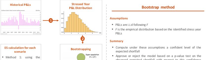
© Global Research & Analytics Dept.| 2018 | All rights reserved

           extracted from the historical observation period. The potential effect of each component
           of the portfolio on the overall portfolio value is then worked out from the component’s
           delta (with respect to a particular risk factor) and that risk factor’s volatility.
      2. Historical VaR: this method is the most frequently used method in banks. It consists in
         applying historical shocks on risk factors to yield a P&L distribution for each scenario
         and then compute the percentile.
      3. Monte-Carlo VaR: this approach consists in assessing the P&L distribution based on
         a large number of simulations of risk factors. The risks factors are calibrated using
         historical data. Each simulation will be different but in total the simulations will
         aggregate to the chosen statistical parameters.

For more details about these three methods, one can refer to the Chappuis Halder & Co.’s white
paper1 on the Value-at-Risk.
Other methods such as “Exponentially Weighted Moving Average” (EWMA), “Autoregressive
Conditional Heteroskedasticity” (ARCH) or the “declined (G)ARCH (1,1) model” exist but are
not addressed in this paper.

           2.1.4. VaR Back-Testing
As mentioned earlier, financial institutions are required to use specific risk measures for Capital
requirements. However, they must also ensure that the models used to calculate these risk
measures are accurate. These tests, also called back-testing, are therefore as important as the
value of the risk measure itself. From a regulatory point of view, the back-testing of the risk
measure used for Capital requirements is an obligation for banks.
However, in the case of the ES for which no sound back-testing methods have yet been found,
regulators had to find a temporary solution. All this lead to the paradoxical situation where the
ES is used for Capital requirements calculations whereas the back-testing is still being
performed on the VaR. In its Fundamental Review of the Trading Book (FRTB), the Basel
Committee includes the results of VaR back-testing in the Capital calculations as a multiplier.
Financial institutions are required to back-test their VaR at least once a year, and on a period of
1 year. The VaR back-testing methodologies used by banks mostly fall into 3 categories of
tests: coverage tests (required by regulators), distribution tests, and independence tests
(optional).
Coverage tests: these tests assess if the number of exceedances during the tested year is
consistent with the quantile of loss the VaR is supposed to reflect.
Before going into details, it seems important to explain how this number of exceedances is
computed. In fact, each day of the tested year, the return of the day [t] is compared with the
calculated VaR of the previous day [t-1]. It is considered an exceedance if the t return is a loss

1
    Value-at-Risk: Estimation methodology and best practices.
                                                        7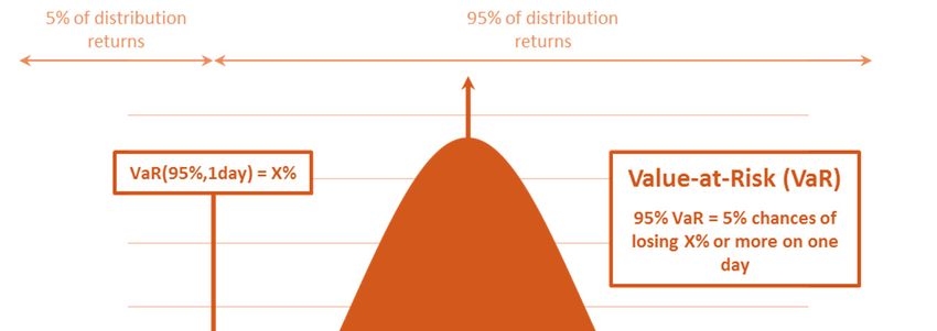
© Global Research & Analytics Dept.| 2018 | All rights reserved

greater than the t-1 VaR. At the end of the year, the total number of exceedances during the
year can be obtained by summing up all exceedances occurrences.
The main coverage tests are Kupiec’s “proportion of failures” (PoF)1 and The Basel
Committee’s Traffic Light coverage test. Only the latter will be detailed here.
The Traffic Light coverage test dates back to 1996 when the Basel Committee first introduced
it. It defines “light zones” (green, yellow and red) depending on the number of exceedances
observed for a certain VaR level of confidence. The colour of the zone determines the amount
of additional capital charges needed (from green to red being the most punitive).

                                               Exceptions           Cumulative
                                  Zone
                                                (out of 250)        probability
                                                     0                 8.11%
                                                     1                 28.58%
                                  Green              2                 54.32%
                                                     3                 75.81%
                                                     4                 89.22%
                                                     5                 95.88%
                                                     6                 98.63%
                                 Yellow              7                 99.60%
                                                     8                 99.89%
                                                     9                 99.97%
                                   Red               10                99.99%

                 Table 1 - Traffic Light coverage test (Basel Committee, 1996), with a coverage of 99%

Ex: let’s say a bank chooses to back-test its 99% VaR using the last 252 days of data. It observes
6 exceedances during the year. The VaR measures therefore falls into the “yellow zone”. The
back-test is not rejected but the bank needs to add a certain amount of capital.
Distribution tests: these tests (Kolmogorov-Smirnov test, Kuiper’s test, Shapiro-Wilk test,
etc.) look for the consistency of VaR measures through the entire loss distribution. It assesses
the quality of the P&L distribution that the VaR measure characterizes.
Ex: instead of only applying a simple coverage test on a 99% quantile of loss, we apply the
same coverage test on different quantiles of loss (98%, 95%, 90%, 80%, etc.)
Independence tests: these tests assess some form of independence in a Value-at-Risk
measure’s performance from one period to the next. A failed independence test will raise doubts
on a coverage or distribution back-test results obtained for that VaR measure.

1
  Kupiec (1995) introduced a variation on the binomial test called the proportion of failures (PoF) test. The PoF
test works with the binomial distribution approach. In addition, it uses a likelihood ratio to test whether the
probability of exceptions is synchronized with the probability “p” implied by the VaR confidence level. If the data
suggests that the probability of exceptions is different than p, the VaR model is rejected.
                                                          8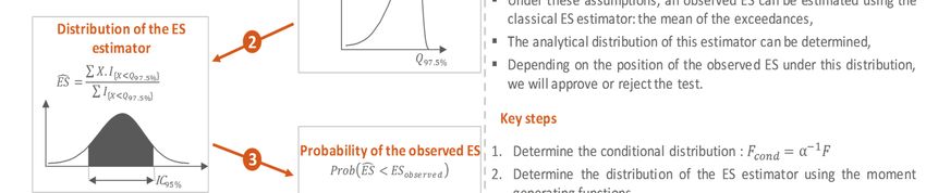
© Global Research & Analytics Dept.| 2018 | All rights reserved

To conclude, in this section were presented the different methodologies used for VaR
calculation and back-testing. However, this risk measure has been widely criticized during the
past years. Among the different arguments, one can notice its inability to predict or cover the
losses during a stressed period, the 2008 crisis unfortunately revealing this lack of efficiency.
Also, its incapacity to predict the tail loss (i.e. extreme and rare losses) makes it difficult for
banks to predict the severity of the loss encountered. The BCBS therefore decided to retire the
well-established measure and replace it by the Expected Shortfall. The following section will
aim at describing this new measure and explain how it defers from the VaR.

   2.2. Expected Shortfall
The Expected Shortfall (ES), aka Conditional VaR (CVaR), was first introduced in 2001 as a
more coherent method than the VaR. The following years saw many debates comparing the
VaR and the ES but it’s not until 2013 that the BCBS decided to shift and adopt ES as the new
risk measure.
In this section are presented the different methodologies of ES calibration and the main
differences between the ES and the VaR. Finally, an introduction of the main issues concerning
the ES back-testing will be made, which will be the focus of the following chapter.

       2.2.1. ES Definition
FRTB defines the ES as the “expected value of those losses beyond a given confidence level”,
over certain time horizon. In other words, the t-ES gives the average loss that can be expected
in t-days when the returns are above the t-VaR.
For example, let’s assume a Risk Manager uses the historical VaR and ES. The observed 97.5%
VaR is $1,000 and there were 3 exceedances ($1,200; $1,100; $1,600). The calibrated ES is
therefore $1,300.

                ES97,5

                                    VaR97,5

                             Figure 2 – Expected shortfall (97.5%) illustration

                                                     9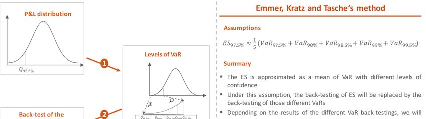
© Global Research & Analytics Dept.| 2018 | All rights reserved

       2.2.2. ES Regulatory framework
The Basel 3 accords introduced the ES as the new measure of risk for capital requirement. As
for the VaR, the parameters for ES calculation are fixed by the regulators. The following table
highlights the regulatory requirements for the ES compared with those of the VaR.

                                       VaR                       Expected Shortfall
          Confidence Level             99%                       97.5%
          Time Horizon                 10 days                   10 days
          Frequency of calculation     Daily                     Daily
          Historical Data              1 previous year           1 stressed year
          Back-Test                    Yes                       Not for the moment

One can notice that the confidence level is lower for the ES than for the VaR. This difference
is due to the fact that the ES is systematically greater than the VaR and keeping a 99%
confidence level would have been overly conservative, leading to a much larger capital reserve
for banks.

       2.2.3. ES Calculation
The calibration of ES is based on the same methodologies as the VaR’s. It mainly consists in
estimating the right P&L distribution, which can be done using one of the 3 following methods:
variance-covariance, historical and Monte-Carlo simulations. These methodologies are
described in part 2.1.2.
Once the P&L distribution is known, the Expected Shortfall is calculated as the mean of returns
exceeding the VaR.
                                              1
                               ∝,  = −
                                             1−∝ ∝
Where :
   -   X is the P&L distribution;

       ∝ is the confidence level;
   -   t is the time point;

        ∝ is the inverse of the VaR function of X at a time t and for a given ∝ confidence
   -
   -
       level.
One must note that the ES is calibrated on a stressed period as it is actually a stressed ES in the
FRTB. The chosen period corresponds to the worst 250 days for the bank’s current portfolio in
recent memory.

                                                10
© Global Research & Analytics Dept.| 2018 | All rights reserved
2.2.4. VaR vs. ES
This section aims at showing the main differences (advantages and drawbacks) between the
VaR and the ES. The following list is not exhaustive and will be summarized in Table 2:
• Amount: given a confidence level X%, the VaR X% is always inferior to the ES X%,
due to the definition of ES as the mean of losses beyond the VaR. This is, in fact, the
reason why the regulatory confidence level changed from 99% (VaR) to 97.5% (ES), as
banks couldn’t have coped with such a high amount of capital otherwise.
• Tail loss information: as mentioned earlier, one of the main drawbacks of the VaR is
its inability to predict tail losses. Indeed, the VaR predicts the probability of an event
but does not consider its severity. For example, a 99% VaR of 1 million predicts that
during the following 100 days, 1 loss will exceed 100k, but it doesn’t make any
difference between a loss of 1.1 million or 1 billion. The ES on the other hand is more
reliable as it does give information on the average amount of the loss than can be
expected.
• Consistency: the ES can be shown as a coherent risk measure contrary to the VaR. In
fact, the VaR lacks a mathematical property called sub-additivity, meaning the sum of
risk measures (RM) of 2 separate portfolios A and B should be equal or greater than the
+
! ≥
#!
risk measure of the merger of these 2 portfolios.
However, in the case of the VaR, one can notice that it does not always satisfy this
property which means that in some cases, it does not reflect the risk reduction from
diversification effects. Nonetheless, apart from theoretical cases, the lack of sub-
additivity of the VaR rarely seems to have practical consequences.
• Stability: the ES appears to be less stable than the VaR when it comes to the distribution.
For fat-tailed distributions for example, the errors in estimating an ES are much greater
than those of a VaR. Reducing the estimation error is possible but requires increasing
the sample size of the simulation. For the same error, an ES is costlier than the VaR
under a fat-tailed distribution.
• Cost / Time consumption: ES calibration seems to require more time and data storage
than the VaR’s. First, processing the ES systematically requires more work than
processing the VaR (VaR calibration being a requirement for ES calculation). Second,
the calibration of the ES requires more scenarios than for the VaR, which means either
more data storage or more simulations, both of which are costly and time consuming.
Third, most banks don’t want to lose their VaR framework, having spent vast amount
of time and money on its development and implementation. These banks are likely to
calculate the ES as a mean of several VaR, which will heavily weigh down calibration
time.
• Facility to back-test: one of the major issue for ES is its difficulty to be back-tested.
Research and financial institutions have been exploring this subject for some years now
but still struggle to find a solution that is both mathematically consistent and practically
implementable. This difficulty is mainly due to the fact that ES is characterised as
“model dependant” (contrary to the VaR which is not). This point is to be explained in
the following section.
11© Global Research & Analytics Dept.| 2018 | All rights reserved
• Elicitability: The elicitability corresponds to the definition of a statistical measure that
allows to compare simulated estimates with observed data. The main purpose of this
measure is to assess the relevance and accuracy of the model used for simulation. To
achieve this, one will introduce a scoring function S(x, y) which is used to evaluate the
performance of x (forecasts) given some values on y (observations). Examples of
scoring functions are squared errors where S(x, y) = (x−y)² and absolute errors where
S(x, y) = |x − y|. Given this definition and due to the nature of the Expected Shortfall,
one will understand that the ES is not elicitable since there is no concrete observed data
to be compared to the forecasts.
VaR ES
Originally greater than the VaR,
but change of regulatory
Amount -
confidence level from 99% to
97.5%
Tail loss Does not give information on the Gives the average amount of the
information severity of the loss loss that can be expected
Lack of sub-additivity:
Consistency Consistent
VaR1+2 > VaR1 + VaR2
Less stable: the estimation error
Stability Relatively stable
can be high for some distribution
Cost / Time
- Always greater than the VaR's
consumption
Difficult to back-test due mainly
Facility to
Easy to back-test due to the fact that the back-
back-test
testing of ES is model dependant
Elicitability Is elicitable Isn’t elicitable
Table 2 - VaR versus ES: main advantages and drawbacks
2.2.5. ES Back-Testing
As mentioned above, the main issue with the ES is its difficulty to be back-tested. Although
research and institutions have already been searching for solutions to this issue for more than
10 years now, no solution seems to satisfy both mathematical properties and practical
requirements. Moreover, following the FRTB evolution and its change from VaR to ES for
Capital requirements, it has become a priority to be consistent in the use of risk measure (i.e.
using the same measure for both Capital calculations and back-testing).
One can wonder why the ES is so difficult to back-test. The main issue is due to the fact that
ES back-testing is characterized as model dependent, unlike the VaR which is model
independent. Both notions will be described in the following paragraphs.
Let’s consider the traditional VaR back-testing and why it is not applicable to the ES. When
back-testing VaR, one would look each day at the return “t” to see if it exceeded the VaR[t-1].
12© Global Research & Analytics Dept.| 2018 | All rights reserved
The number of exceedances, corresponding to the sum of exceedance occurrences, would then
be compared to the quantile the VaR is supposed to reflect.
If one considers that the P&L distribution is likely to change over time, the VaR levels, to which
the returns are compared with, also change over time. One would therefore look at the number
of exceedances over a value that possibly changes every day. To illustrate this point, the exact
same return could be considered as an exceedance one day, and not on another day.
When back-testing the VaR, although the reference value (i.e. the VaR) changes over time,
calculating the total number of exceedances still makes sense as one can find convergence of
the results. This mathematical property characterizes the VaR back-testing as model
independent: results are still consistent when the P&L distribution changes during the year.
In the case of the ES however, one would not only look at the number of exceedances but also
their values. This additional information complicates the task as there is no convergence when
looking at the mean of the exceedances. To make sense, the P&L distribution (or more exactly
the VaR) should remain constant during the time horizon. The back-testing of ES is therefore
characterized as model dependent.
The characterization of ES back-testing as model dependent is one of the main issue that
financial institutions experience. Unlike the VaR, they cannot only compare the theoretical ES
with the observed value at the end of the year since in most cases the later value does not make
sense.
This constraint, combined with limitations in both data storage and time-implementation, makes
it difficult for financial institutions and researchers to find new ways to back-test the ES.
The following section aims at presenting the main results and findings of the last 10 years of
research and presents alternative solutions introduced by the Global Research & Analytics team
of Chappuis Halder & Co.
13© Global Research & Analytics Dept.| 2018 | All rights reserved
3. ES Back-Testing
As mentioned earlier, the purpose of this chapter is to present the latest developments in terms
of ES back-testing methodologies and to introduce new methodologies developed by the Global
Research & Analytics (GRA) team of Chappuis Halder & Co.
3.1. Existing Methods
3.1.1. Wong’s Saddle point technique
Wong (2008) proposed a parametric method for the back-testing of the ES. The purpose of the
methodology is to find the probability density function of the Expected Shortfall, defined as a
mean of returns exceeding the VaR. Once such distribution is found, one can find the
confidence level using the Lugannani and Rice formulas, which provide the probability to find
a theoretical ES inferior to the sample (i.e. observed) ES. The results of the back-test depend
on this “p-value”: given a confidence level of 95%, the p-value must be at least superior to 5%
to accept the test.
The method relies on 2 major steps:
1. Inversion formula: find the PDF knowing the moment-generating function
2. Saddle point Technique to approximate the integral
Figure 3 - Overview of Wong's Approach
The ideas of the parametric method proposed by Wong (2008) are as follows. Let
$ , % , & … ( be the portfolio returns which has predetermined CDF and PDF denoted by φ
and ) respectively. We denote by q φ + the theoretical α-quantile of the returns.
The statistic used to determine the observed expected shortfall is the following:
4
. /$0123(
, = −- = − 5
4
. /$0123(
5
Where / $623( is the logical test whether the value x is less than the , 7
The purpose of this method is to analytically estimate the density of this statistic and then see
where is positioned the observed value with respect to this density.
14© Global Research & Analytics Dept.| 2018 | All rights reserved
4
Are denoted by 8, the realised quantity . /$0123( which is the number of exceedances
5
observed in our sample, and 9 the realised return exceedances below the +-quantile q. The
observed expected shortfall is then:
∑>5
:,
−;̅ −
8
Reminder of the moment-generating function:
The moment-generating function (MGF) provides an alternative way for describing a random
variable, which completely determines the behaviour and properties of the probability
distribution of the random variable X:
? 9 @AB ? C
The inversion formula that allows to find the density once we have the MGF is the following:
1 I FG (1.1)
)? 9 B
? H
2E I
One of the known features of the moment-generating function is the following:
? + + JK
? +9 ∙
M J9 (1.2)
Let be a continuous random variable with a density + );, ; ∊ −∞, 7. The moment
PROPOSITION 1:
generating function of is then given by:
? 9 = + B;P9 % ⁄2)7 − 9 (1.3)
and its derivatives with respect to 9 are given by:
?R 9 = 9 ∙
? 9 − + ∙ B;P79 ∙ )7
RR 9
? = 9 ∙
?R 9 +
? 9 − 7 + ∙ B;P79 ∙
(1.4)
)7 (1.5)
S S
? 9 9 ∙
? 9 + T − 1
?S 9 − 7 S + ∙ B;P79 ∙ )7 (1.6)
where T ≥3
Using these, we can also show that the mean and variance of can be obtained easily:
)7
U? = @AC = −
+
7)7
V?% = WXAC = 1 − − U?%
+
The Lugannani and Rice formula
function of the statistic - (1.1).
Lugannani and Rice (1980) provide a method which is used to determine the cumulative density
15© Global Research & Analytics Dept.| 2018 | All rights reserved
It is supposed that the moment-generating function of the variable = /$0123( is known.
]
Using the property (1.2), one can compute
YZ 9 = [
? \ ^_ and via the inversion formula
]
1 I F` 9 8 I ]cAFCF`
]
will obtain:
)YZ ; = B a
? [H _b
9 = B
9
2E I 8 2E I
where )YZ ; denotes the PDF of the sample mean and dA9C = e8
? A9C is the cumulative-
generating function of )? ;. Then the tail probability can be written as:
g
1 Ω#FI
9
- > ;̅ = )YZ 9
9 = B ]cAC`̅
`̅ 2E H ΩFI 9
where Ω is a saddle-point1 satisfying:
d R Ω = ;̅ (1.9)
The saddle-point is obtained by solving the following expression deduced from (1.4) and (1.5):
R Ω )7
d R Ω = = Ω − exp7Ω − Ω% ⁄2 = ;̅
Ω φq − Ω
(1.10)
Finally, Lugannani and Rice propose to approximate this integral as follows:
PROPOSITION 2:
Let Ω be a saddle-point satisfying the equation (1.9) and define:
i = Ω j8d RR Ω
:, − dΩ^
k = lm8Ωn28 \Ω
where lm8Ω equals to zero when Ω = 0, or takes the value of 1/−1) when Ω < 0/Ω > 0).
Then the tail probability of ;̅ less than or equal to the sample mean ;̅ is given by
1 1
v φk − )k ∙ a − + wx8&⁄% yb )zX ;̅ < 7 8
;̅ ≠ U?
t i k
t
1 )zX Z; > 7
- ≤ ;̅ =
u 1 d 0
&
t − + + wx8&⁄% y )zX ;̅ = U?
t 2
6n2E8xd RR Ωy
&
s
1
In mathematics, a saddle point or minimax point is a point on the surface of the graph of a function where the
slopes (derivatives) of orthogonal function components defining the surface become zero (a stationary point) but
are not a local extremum on both axes.
16© Global Research & Analytics Dept.| 2018 | All rights reserved
Once the tail probability is obtained, one can compute the observed expected shortfall :, and
carry out a one-tailed back-test to check whether this value is too large. The null and alternative
hypotheses can be written as:
:, = -----
, :, > -----
,
H0: versus H1:
where -----
, denotes the theoretical expected shortfall under the null hypothesis.
The p-value of this hypothesis test is simply given by the Lugannani and Rice formula as
P G = - ≤ ;̅
Example:
For a portfolio composed of one S&P500 stock, it is assumed that the bank has predicted that
the daily P&L log-returns are i.i.d and follow a normal distribution calibrated on the
can consider that the sample follows a standard normal distribution 0,1. Using Wong’s
observations of the year 2014. Then all the observations of the year 2015 are normalised so one
method described above, the steps to follow in order to back-test the under these
assumptions and with + = 2.5% are:
1. Calculate the theoretical +-quantile: 7 = −φ 2.5% = 1.96
2. Calculate the observed ES of the normalized log-returns of 2015: - = −2.84, 8 = 19
3. Solve the equation (1.10) to find the saddle-point: Ω = −3.23
4. Calculate dAΩC and d RR AΩC where
R 9
RR 9
9 −
R 9%
d RR AtC = =
9
9
9%
RR AΩC
In our case, we found: dAΩC = 8.80 and d = 2.49
:
5. Calculate the tail probability of and compare to the level of confidence tolerated
,
by the P G test: x, ≤ :, y~0
In this example, the null hypothesis is rejected. Not only does it show that the movements of
2015 cannot be explained by the movements of 2014, but it also shows that the hypothesis of a
normal distribution of the log-returns is not likely to be true.
3.1.2. Righi and Ceretta
The method of Righi and Ceretta is less restrictive than Wong’s one in the sense that the law of
the returns may vary from one day to another. However, it requires the knowledge of the
truncated distribution below the negative VaR level.
17© Global Research & Analytics Dept.| 2018 | All rights reserved
Figure 4 - Righi and Ceretta - Calculating the Observed statistic test
Figure 5 - Righi and Ceretta - Simulating the statistic test
Figure 6 - Righi and Ceretta – Overview
18© Global Research & Analytics Dept.| 2018 | All rights reserved
conditional heteroscedastic xP, 7y model, which are largely applied in finance:
In their article, they consider that the portfolio log-returns follow generalized autoregressive
X = U + , = V
V = ω + . F F + . J V %
% %
g
where X is the log-return, U is the conditional mean, V is the conditional variance and is the
shock over the expected value of an asset in period t; , and J are parameters; represents
denoted respectively and ) .
the white noise series which can assume many probability distribution and density functions
distribution properties, mainly the + − quantile/ES:
The interest behind using this model is mainly the fact that we can easily predict the truncated
,, = U + V +
= U + V @A | < +C (2.1)
But one can also calculate the dispersion of the truncated distribution as follows:
¢ = nXxU + V £ < +y = V nXx £ < +y (2.2)
The ES and SD are mainly calculated via Monte-Carlo simulations. In some cases, it is possible
to have their parametric formulas:
1. Case where ¤¥ is normal |
It is assumed that is a standard Gaussian noise 0,1, which is a very common case. The
)
expectation of the truncated normal distribution is then:
@A | < C =
substituting this expression in the equation of (2.1), it is obtained:
) \ ¦ +^
= U + V
+
) ) %
The variance of a truncated normal distribution below a value is given by:
A | < C = 1− −[ _
Substituting this expression in the variance term of the formula (2.2), it is deduced:
+ + % %
) )
¢ = V ∙ §1 − + −a b ¨
+ +
2. Case where ¤¥ follows a Student’s distribution |
19© Global Research & Analytics Dept.| 2018 | All rights reserved
It is assumed that is a Student’s 9 distributed random variable with W degrees of freedom.
One can show that the truncated expectation is as follow:
1 1+W %
@A | < C = © %
a , 1; 2; − b«
W 1 2 2
2√W J \ , ^
2 2
substituting this expression in the expectation of (1), it is obtained:
1 +%
1+W +%
= U + V ¬ © a , 1; 2; − b«
W 1 2 2
2√W+ ∙ J \2 , 2^
where J∙,∙ and ∙ , ∙ ; ∙ ; ∙ are the Beta and Gauss hyper geometric functions conform to:
1
J, ® =
−
¯
°
² ®² ²
I
, ®; ±; = .
±² ³!
²5°
Where ∙² denotes the ascending factorial.
Similarly, for the standard normal SD, it is deduced from the variance of a truncated Student’s
t distribution:
1 1+W 3 5 %
A | < C = Q& a , ; ;− b
W 1 2 2 2 2
3√W J \2 , 2^
Again, substituting this variance term in (2.2), one will obtain an analytical form of the standard
deviation of the truncated distribution:
%
+%
1 1+W 3 5
¢ = V ∙ ¶ +& a , ; ;− b·
W 1 2 2 2 2
3√W+ ∙ J \2 , 2^
Once the ED and SD are expressed and computed, for each day in the forecast period for
which a violation in the predicted Value at Risk occurs, the following test statistic is defined:
X −
¸¹ =
¢
(2.3)
− @A | < C
¹ =
jA | < C (2.4)
Where is the realisation of the random variable º (in the Garch process, it is supposed that
º is iid but it is not necessarily the case).
20© Global Research & Analytics Dept.| 2018 | All rights reserved
The idea of Righi and Ceretta is to see where the value of ¸¹ is situated with respect to the
“error” distribution of the estimator ¹ = 1
» @A»1 |»1 2¼C
j½ 0A»1 |»1 2¼C
ℙ¹ < ¸¹ and then take the median (or eventually the average) of these probabilities over
by calculating the probability
the time as a p-value over a certain confidence level P.
They propose to calculate this distribution using Monte-Carlo simulations following this
1) Generate times a sample of 8 − HH
random variable
F under the distribution , H =
algorithm:
1, … , 8; ¿ = 1, … , ;
2) Estimating for each sample the quantity @À
F |
F < 7x
F yÁ and À
F |
F <
7x
F yÁ where 7x
F y is the +-th worst observation over the sample
F
3) Calculate for each realisation
F , the quantity ℎF =
GÃÄ @ÀGÃÄ |GÃÄ 2gxGÃÄ yÁ
n½ 0ÀGÃÄ |GÃÄ 2gxGÃÄ yÁ
which is a
realisation of the random variable ¹ defined above.
4) Given the actual ¸¹ , estimate ℙ < ¸¹ using the sample ℎF as an empirical
distribution of
5) Determine the test p-value as the median of ℙ < ¸¹ and compare the value to the
test level fixed at P.
2014 to 2015 year. The results, where is a standard Gaussian noise 0,1, are the following:
The methodology has been applied on the test portfolio of the normalized daily returns for the
Distribution* Standard Normal
Level of freedom* none
Inputs
Confidence Level of the ES* 97,5%
Scenario 05/08/2014
VaRth 1,96
ESth 2,34
VaRobs 2,38
Number of exceedances 12
ESobs 2,49
BT Results var(X© Global Research & Analytics Dept.| 2018 | All rights reserved
In the table below are displayed the exceedance rates and the associated test statistics:
Exceedance # Exceedance Value Test statistic P(Ht© Global Research & Analytics Dept.| 2018 | All rights reserved
3.1.4. Summary of the methods
In this section, it is summarised the three different methods in term of application and
implementation as well as their drawbacks:
Wong’s method |
Figure 7 - Summary of Wong’s methodology
23© Global Research & Analytics Dept.| 2018 | All rights reserved
Righi and Ceretta Method |
Figure 8 - Summary of Righi and Cereta’s methodology
Emmer, Kratz and Tasche Method |
Figure 9 - Summary of Emmer, Kratz and Tasche’s methodology
24© Global Research & Analytics Dept.| 2018 | All rights reserved
3.2. Alternative Methods
In the following sections are presented alternative methods introduced by the Global Research
& Analytics (GRA) department of Chappuis Halder &Co.
First of all, it is important to note that some of the following methods rely on a major hypothesis,
which is the consistency of the theoretical VaR for a given period of time. This strong – and
not often met - assumption is due to the use of what is called “observed ES”.
The observed ES reflects the realised average loss (above the 97.5% quantile) during a 1-year
time period as illustrated in the below formula:
∑%È°
5 # /# >
ͯ
Where corresponds to the return day 9 and is the number of exceedances during the year
( ∑%È°
5 /# > with / the identity function) .
1
However, this value only makes sense as long as the theoretical VaR (or more broadly the P&L
distribution used for calibration) doesn’t change during this time period. Should the opposite
occur, one would look at the loss beyond a level that changes with time, and the average of
these losses would lose any meaning.
3.2.1. ES Benchmarking
This method focuses on the distance Î − ͯ between the theoretical ES (obtained by
calibration) and the observed ES (corresponding to realised returns). The main goal of this
methodology is to make sure the distance Î − ͯ (back-testing date) is located within
the confidence interval. This interval can be found by recreating a distribution from historical
values. The output of the back-test depends on the position of the observed distance: if the value
is within the interval, the back-test is accepted, otherwise it is rejected.
The historical distribution is based on 5 years returns (i.e. 5*250 values). For each day of these
5 years, the distance Î − ͯ , Î and ͯ is calculated as described in the introduction
of this section. The 1,250 values collected can therefore be used to build a distribution that fits
historical behaviour.
1
As mentioned in part 2.1.1, VaR is calculated with a 1-day time horizon. Therefore, the return that is compared
to the VaR[t] is the return X[t+1]
25© Global Research & Analytics Dept.| 2018 | All rights reserved
Figure 10 - Illustration of ES Benchmarking Methodology
One of the main downside of the methodology is that it relies on the notion of observed ES.
However, as mentioned earlier, this particular value requires a constant VaR, which is not often
met in reality.
Finally, once the confidence interval is obtained, one can used it in order to back-test the
simulated ES on the future back-testing horizon.
3.2.2. Bootstrap
This methodology focuses on the value of the observed ES. As for the previous methodology,
the goal of this method is to verify that the observed ES is located within the confidence interval.
The latest can be found by recreating a distribution from historical values using the bootstrap
approach which is detailed below. The output of the test depends on the position of the observed
ES (back-testing date): if the value is in the interval, the back-test is accepted, otherwise it is
rejected.
In this methodology, the bootstrap approach is used to build a more consequent vector of returns
in order to find the distribution of the ES as the annual mean of returns exceeding the VaR. This
approach consists in simulating returns, using only values from a historical sample. The vector
formed by all simulated values therefore only contains historical data that came from the
original sample.
The overall methodology relies in 3 steps as illustrated in Figure 11:
1. The sample vector is obtained and contains the returns of 1-year data;
2. Use of the bootstrap method to create a bigger vector, filled only with values from the
sample vector. This vector will be called the “Bootstrap Vector”;
3. The final vector, used for compiling the distribution, is obtained by selecting only
returns exceeding the VaR from the bootstrap vector;
4. The distribution can be reconstructed, using the final vector.
26© Global Research & Analytics Dept.| 2018 | All rights reserved
Figure 11 - Illustration of Bootstrap Methodology
3.2.3. Quantile Approaches
Whereas the Expected Shortfall is usually expressed as a value of the loss (i.e. in £, $, etc.), the
two methodologies Quantile 1 and Quantile 2 choose to focus on the ES as a quantile, or a
probability value of the P&L distribution. The two methods differ in the choice of the quantile
adopted for the approach.
The following paragraphs describe the two different options for the choice of the quantile.
Quantile 1
This methodology focuses on the quantile of the observed ES (back-testing date), in other words
the answer to the question: “which probability is associated to the value of a specific Expected
Shortfall in the P&L distribution?”
One must notice that this quantile is not the confidence level of the Expected Shortfall. Indeed,
let’s take a confidence level of 97.5% as requested by the regulation. It is possible to estimate
an observed VaR and therefore an observed ES as a mean of returns exceeding the VaR. The
observed quantile can be found by looking at the P&L distribution and spotting the probability
associated to the ES value. The ES being strictly greater than the VaR, the quantile will always
be strictly greater than 97.5%.
Figure 12 - Calculation of the Quantile Q1
Quantile 2
This methodology looks at the stressed-retroactive quantile of the observed ES (back-testing
date), that is to say the answer to the question: “To which quantile correspond the observed ES
27© Global Research & Analytics Dept.| 2018 | All rights reserved
at the time of the back-testing if it was observed in the reference stressed period used for
calibration?”
Figure 13 - Calculation of the quantile Q2
Back-testing methodology
Once the choice of the quantile computation is done, the approach is the same for the two
methodologies: it consists in verifying that the calculated quantile at the date of the back-testing
is located in the confidence interval obtained from a reconstructed historical distribution. If the
quantile is within the confidence interval, the back-test is accepted, otherwise it is rejected.
The distribution is obtained using the same framework as for the ES Benchmarking
methodology (see Section 3.2.1). The quantile is computed each day over 5 years (for the first
method the observed quantile and for the second one, the stressed-retroactive quantile). Those
1,250 values are used to build a historical distribution of the chosen quantile and the confidence
interval immediately follows.
Figure 14 - Illustration of the Quantile 1 Methodology
3.2.4. Summary of the methods
ES Benchmarking |
28© Global Research & Analytics Dept.| 2018 | All rights reserved
Figure 15- Summary of the ES Benchmarking methodology
Quantile method |
Figure 16 - Summary of the Quantile methodology
29© Global Research & Analytics Dept.| 2018 | All rights reserved
Bootstrap method |
Figure 17 - Summary of the Bootstrap methodology
30© Global Research & Analytics Dept.| 2018 | All rights reserved
4. Applications of the ES methodology and back-testing
4.1. ES simulations
In this section, the back-testing approaches presented in the 3.2 section have been applied
on simulations of the S&P 500 index1. Indeed, instead of performing back-testing on
parametric distributions; it has been decided to perform a back-testing exercise on simulated
values of an equity (S&P 500 index) based on Monte Carlo simulations. The historic levels of
the S&P 500 are displayed in Figure 18 below:
S&P 500 Level - January 2011 to December 2015
S&P 500 Level
2 400
2 200
2 000
1 800
1 600
1 400
1 200
1 000
Figure 18 - S&P 500 Level – From January 2011 to December 2015
A stochastic model has been used in order to forecast the one-day return of the stock price
which has been compared to the observed returns. The stochastic model relies on a Geometric
Brownian Motion (hereafter GBM) and the simulations are done with a daily reset as it
could be done in a context of Market Risk estimation.
The stochastic differential equation (SDE) of a GBM in order to diffuse the stock price is as
follows:
U
9 + V
Ï
And the closed form solution of the SDE is:
ÒÓ
Ð[Ñ _#ÒÔÕ
9 0B %
Where:
− S is the Stock price
1
The time period and data selected (from January 2011 to December 2015) is arbitrary and one would obtain
similar results and findings with other data.
31© Global Research & Analytics Dept.| 2018 | All rights reserved
U is the expected return
V is the standard deviation of the expected return
−
9 the time
−
Ï9 is a Brownian Motion
−
−
Simulations are performed on a day-to-day basis over the year 2011 and 1,000 scenarios are
produced per time points. Therefore, thanks to these simulations, it is possible to compute
a one-day VaR99% as well as a one-day ES97.5% of the return which are then compared to
the observed return price.
Both VaR and ES are computed as follows:
FS 9
− ͯ 9 − 1
ÊÊ% 9 a b
ÊÊ%
ͯ 9 − 1
− ͯ 9 − 1
FS 9
_ I ØÙÃÚ ØÛÜÙ
ͯ 9 − 1
∑]F5 [
× Ý½ 0Þß.à% á
ÊË.È% 9
Ø ÛÜÙ
∑]F5 I ØÙÃÚ ØÛÜÙ
ݽ 0Þß.à% á
ØÛÜÙ
×
Where n is the total number of scenarios per time point t.
The figure below shows the results of our simulations and computations of the VaR99% and
ES97.5%:
S&P 500 - Observed vs. Simulations
returns 1d VaR - 99% ES - 97,5%
6,0%
4,0%
2,0%
0,0%
-2,0%
-4,0%
-6,0%
-8,0%
Figure 19 - Observed returns vs. simulations – From January 2011 to January 2012
32© Global Research & Analytics Dept.| 2018 | All rights reserved
Figure 19 shows that in comparison to the observed daily returns, the VaR99% and the ES97,5%
gives the same level of conservativeness. This is further illustrated with Figure 20 where it is
observed that the level of VaR and Expected shortfall are close.
S&P 500 - Comparison of the VaR with the ES
VaR - 99% ES - 97,5%
-1,7%
-1,8%
-1,9%
-2,0%
-2,1%
-2,2%
-2,3%
-2,4%
-2,5%
-2,6%
-2,7%
Figure 20 – Comparison of the VaR99% with the ES97.5% - From January 2011 to January 2012
When looking at Figure 20, one can notice that the ES97.5% doesn’t always lead to more
conservative results in comparison to the VaR99%. This is explained by the fact that the ES is
the mean of the values above the VaR97.5%, consequently and depending on the Monte Carlo
simulations it is realistic to observe ES97.5% slightly below the VaR99%.
Finally, when looking at the simulations, one can conclude that both risk measures are really
close. Indeed the distribution of the spread between the simulated VaR99% and the ES97.5% (see
Figure 21 below); it is observed that 95% of the spread between both risk measures are within
the ]-0.1%, 0.275%] interval.
33© Global Research & Analytics Dept.| 2018 | All rights reserved
Distribution of the spread of the (VaR99% - ES97,5% ) - From January
2011 to December 2015
18% 18%
15%
13%
11%
8%
5%
3%
2% 2% 1%
1% 0% 1% 1% 1% 0% 0% 0% 0%
(VaR99% - ES97,5% )
Figure 21 – Spread VaR99% vs. ES97.5% - January 2011 to September 2015
Following the computation of these simulated ES, it can be concluded that in comparison
to a VaR measure, the ES is not overly conservative and severe measure. Given these
findings and knowing that the ES is a more consistent measure in comparison to the VaR (due
to the way it is estimated), it can be accepted as a suitable risk measure provided that a reliable
approach is used in order to back-test the results.
4.2. Back-test of the ES using our alternative methods
Following the previous conclusions, it has been decided to focus on some approaches
defined in section 3.2. That’s why an observed ES has been computed based on the daily
VaR97.5% (obtained via the MC simulations) and the observed returns over the year following
the simulation date. Its expression is as follows:
∑S
F5 9 + HI$0#Fݽ 0Þß.à% (
ͯ 9
∑SF5 I$0#Fݽ 0Þß.à% (
Where m is the number of days in the year following the date t and R(t) the daily return observed
at date t:
ͯ 9 − ͯ 9 − 1
ͯ 9 − 1
9
As presented in the section 3.2.1, this observed ES has been compared to the theoretical daily
simulated ES.
34You can also read