Intermediate Value Linearizability: A Quantitative Correctness Criterion - Schloss Dagstuhl
←
→
Page content transcription
If your browser does not render page correctly, please read the page content below
Intermediate Value Linearizability: A Quantitative
Correctness Criterion
Arik Rinberg
Technion – Israel Institute of Technology, Haifa, Israel
ArikRinerg@campus.technion.ac.il

Idit Keidar
Technion – Israel Institute of Technology, Haifa, Israel
idish@ee.technion.ac.il

      Abstract

Big data processing systems often employ batched updates and data sketches to estimate certain
properties of large data. For example, a CountMin sketch approximates the frequencies at which
elements occur in a data stream, and a batched counter counts events in batches. This paper focuses
on correctness criteria for concurrent implementations of such objects. Specifically, we consider
quantitative objects, whose return values are from a totally ordered domain, with a particular
emphasis on (, δ)-bounded objects that estimate a numerical quantity with an error of at most
with probability at least 1 − δ.

     The de facto correctness criterion for concurrent objects is linearizability. Intuitively, under
linearizability, when a read overlaps an update, it must return the object’s value either before the
update or after it. Consider, for example, a single batched increment operation that counts three
new events, bumping a batched counter’s value from 7 to 10. In a linearizable implementation of the
counter, a read overlapping this update must return either 7 or 10. We observe, however, that in
typical use cases, any intermediate value between 7 and 10 would also be acceptable. To capture this
additional degree of freedom, we propose Intermediate Value Linearizability (IVL), a new correctness
criterion that relaxes linearizability to allow returning intermediate values, for instance 8 in the
example above. Roughly speaking, IVL allows reads to return any value that is bounded between
two return values that are legal under linearizability. A key feature of IVL is that we can prove
that concurrent IVL implementations of (, δ)-bounded objects are themselves (, δ)-bounded. To
illustrate the power of this result, we give a straightforward and efficient concurrent implementation
of an (, δ)-bounded CountMin sketch, which is IVL (albeit not linearizable).

    Finally, we show that IVL allows for inherently cheaper implementations than linearizable ones.
In particular, we show a lower bound of Ω(n) on the step complexity of the update operation of
any wait-free linearizable batched counter from single-writer objects, and propose a wait-free IVL
implementation of the same object with an O(1) step complexity for update.

2012 ACM Subject Classification Theory of computation → Semantics and reasoning; Computer
systems organization → Parallel architectures; Computing methodologies → Concurrent computing
methodologies

Keywords and phrases concurrency, concurrent objects, linearizability

Digital Object Identifier 10.4230/LIPIcs.DISC.2020.2

Related Version A full version of the paper is available at [31], https://arxiv.org/abs/2006.12889.

Acknowledgements We thank Hagit Attiya and Gadi Taubenfeld for their insightful comments, and
the anonymous reviewers for their detailed feedback.
            © Arik Rinberg and Idit Keidar;
            licensed under Creative Commons License CC-BY
34th International Symposium on Distributed Computing (DISC 2020).
Editor: Hagit Attiya; Article No. 2; pp. 2:1–2:17
                   Leibniz International Proceedings in Informatics
                   Schloss Dagstuhl – Leibniz-Zentrum für Informatik, Dagstuhl Publishing, Germany
2:2 Intermediate Value Linearizability
1 Introduction
1.1 Motivation
Big data processing systems often perform analytics on incoming data streams, and must do
so at a high rate due to the speed of incoming data. Data sketching algorithms, or sketches
for short [6], are an indispensable tool for such high-speed computations. Sketches typically
estimate some function of a large stream, for example, the frequency of certain items [7],
how many unique items have appeared [9, 13, 14], or the top-k most common items [26].
They are supported by many data analytics platforms such as PowerDrill [18], Druid [11],
Hillview [19], and Presto [30] as well as standalone toolkits [10].
Sketches are quantitative objects that support update and query operations, where
the return value of a query is from a totally ordered set. They are essentially succinct
(sublinear) summaries of a data stream. For example, a sketch might estimate the number of
packets originating from any IP address, without storing a record for every packet. Typical
sketches are probably approximately correct (PAC), estimating some aggregate quantity with
an error of at most with probability at least 1 − δ for some parameters and δ. We say
that such sketches are (, δ)-bounded.
The ever increasing rates of incoming data create a strong demand for parallel stream
processing [8, 18]. In order to allow queries to return fresh results in real-time without
hampering data ingestion, it is paramount to support queries concurrently with updates [32,
33]. But parallelizing sketches raises some important questions, for instance: What are
the semantics of overlapping operations in a concurrent sketch?, How can we prove error
guarantees for such a sketch?, and, in particular, Can we reuse the myriad of clever analyses
of existing sketches’ error bounds in parallel settings without opening the black box? In this
paper we address these questions.
1.2 Our contributions
The most common correctness condition for concurrent objects is linearizability. Roughly
speaking, it requires each parallel execution to have a linearization, which is a sequential
execution of the object that “looks like” the parallel one. (See Section 2 for a formal
definition.) But sometimes linearizability is too restrictive, leading to a high implementation
cost.
In Section 3, we propose Intermediate Value Linearizability (IVL), a new correctness
criterion for quantitative objects. Intuitively, the return value of an operation of an IVL
object is bounded between two legal values that can be returned in linearizations. The
motivation for allowing this is that if the system designer is happy with either of the legal
values, then the intermediate value should also be fine. For example, consider a system where
processes count events, and a monitoring process detects when the number of events passes a
threshold. The monitor constantly reads a shared counter, which other process increment in
batches. If an operation increments the counter from 4 to 7 batching three events, IVL allows
a concurrent read by the monitoring process to return 6, although there is no linearization
in which the counter holds 6. We formally define IVL and prove that this property is local,
meaning that a history composed of IVL objects is itself IVL. This allows reasoning about
single objects rather than about the system as a whole. We formulate IVL first for sequential
objects, and then extend it to capture randomized ones.
Next, we consider (, δ)-bounded algorithms like data sketches. Existing (sequential)
algorithms have sequential error analyses which we wish to leverage for the concurrent case. In
Section 4 we formally define (, δ)-bounded objects, including concurrent ones. We then proveA. Rinberg and I. Keidar 2:3
a key theorem about IVL, stating that an IVL implementation of a sequential (, δ)-bounded
object is itself (, δ)-bounded. The importance of this theorem is that it provides a generic
way to leverage the vast literature on sequential (, δ)-bounded sketches [27, 12, 5, 24, 7, 1]
in concurrent implementations.
As an example, in Section 5, we present a concurrent CountMin sketch [7], which estimates
the frequencies of items in a data stream. We prove that a straightforward parallelization of
this sketch is IVL. By the aforementioned theorem, we deduce that the concurrent sketch
adheres to the error guarantees of the original sequential one, without having to “open” the
analysis. We note that this parallelization is not linearizable.
Finally, we show that IVL is sometimes inherently cheaper than linearizability. We
illustrate this in Section 6 via the example of a batched counter. We present a wait-free IVL
implementation of this object from single-writer-multi-reader (SWMR) registers with O(1)
step complexity for update operations. We then prove a lower bound of Ω(n) step complexity
for the update operation of any wait-free linearizable implementation, using only SWMR
registers. This exemplifies that there is an inherent and unavoidable cost when implementing
linearizable algorithms, which can be circumvented by implementing IVL algorithms instead.
2 Preliminaries
Section 2.1 discusses deterministic shared memory objects and defines linearizability. In
Section 2.2 we discuss randomized algorithms and their correctness criteria.
2.1 Deterministic objects
We consider a standard shared memory model [17], where a set of processes access atomic
shared memory variables. Accessing these shared variables is instantaneous. Processes take
steps according to an algorithm, which is a deterministic state machine, where a step can
access a shared memory variable, do local computations, and possibly return some value.
An execution of an algorithm is an alternating sequence of steps and states. We focus on
algorithms that implement objects, which support operations, such as read and write.
Operations begin with an invocation step and end with a response step. A schedule, denoted
σ, is the order in which processes take steps, and the operations they invoke in invoke steps
with their parameters. Because we consider deterministic algorithms, σ uniquely defines an
execution of a given algorithm.
A history is the sequence of invoke and response steps in an execution. Given an algorithm
A and a schedule σ, H(A, σ) is the history of the execution of A with schedule σ. A sequential
history is an alternating sequence of invocations and their responses, beginning with an
invoke step. We denote the return value of operation op with parameter arg in history H by
ret(op, H). We refer to the invocation step of operation op with parameter arg by process
p as invp (op(arg)) and to its response step by rspp (op) → ret, where ret = ret(op, H).
A history defines a partial order on operations: Operation op1 precedes op2 in history H,
denoted op1 ≺H op2 , if rsp(op1 ) precedes inv(op2 (arg)) in H. Two operations are concurrent
if neither precedes the other.
A well-formed history is one that does not contain concurrent operations by the same
process, and where every response event for operation op is preceded by an invocation of
the same operation. A schedule is well-formed if it gives rise to a well-formed history, and
an execution is well-formed if it is based on a well-formed schedule. We denote by H|x the
sub-history of H consisting only of invocations and responses on object x. Operation op is
pending in a history H if op is invoked in H but does not return.
DISC 20202:4 Intermediate Value Linearizability
Correctness of an object’s implementation is defined with respect to a sequential spe-
cification H, which is the object’s set of allowed sequential histories. If the history spans
multiple objects, H consists of sequential histories H such that for all objects x, H|x pertains
to x’s sequential specification (denoted Hx ). A linearization [17] of a concurrent history
H is a sequential history H 0 such that (1) after removing some pending operations from
H and completing others, it contains the same invocations and responses as H 0 with the
same parameters and return values, and (2) H 0 preserves the partial order ≺H . Note that
our definition of linearization diverges from the one in [17] in that it is not associated
with any sequential specification; instead we require that the linearization pertain to the
sequential specification when defining linearizability as follows: Algorithm A is a linearizable
implementation of a sequential specification H if every history of a well-formed execution of
A has a linearization in H.
2.2 Randomized algorithms
In randomized algorithms, processes have access to coin flips from some domain Ω. Every
execution is associated with a coin flip vector #»
c = (c1 , c2 , . . . ), where ci ∈ Ω is the ith coin flip
in the execution. A randomized algorithm A is a probability distribution over deterministic
algorithms {A( #»c )} #» 1
c ∈Ω∞ , arising when A is instantiated with different coin flip vectors. We
#»
denote by H(A, c , σ) the history of the execution of randomized algorithm A observing coin
flip vector #»
c in schedule σ.
Golab et al. show that randomized algorithms that use concurrent objects require a
stronger correctness criterion than linearizability, and propose strong linearizability [15].
Roughly speaking, strong linearizability stipulates that the mapping of histories to lineariza-
tions must be prefix-preserving, so that future coin flips cannot impact the linearization order
of earlier events. In contrast to us, they consider deterministic objects used by randomized
algorithms. In this paper, we focus on randomized object implementations.
3 Intermediate value linearizability
Section 3.1 introduces definitions that we utilize to define IVL. Section 3.2 defines IVL for
deterministic algorithms and proves that it is a local property. Section 3.3 extends IVL for
randomized algorithms, and Section 3.4 compares IVL to other correctness criteria.
3.1 Definitions
Throughout this paper we consider the strongest progress guarantee, bounded wait-freedom.
An operation op is bounded wait-free if whenever any process p invokes op, op returns a
response in a bounded number of p’s steps, regardless of steps taken by other processes. An
operation’s step-complexity is the maximum number of steps a process takes during a single
execution of this operation. We can convert every bounded wait-free algorithm to a uniform
step complexity one, in which each operation takes the exact same number of steps in every
execution. This can be achieved by padding shorter execution paths with empty steps before
returning. Note that in a randomized algorithm with uniform step complexity, coin flips have
no impact on op’s execution times. For the remainder of this paper, we consider algorithms
with uniform step complexity.
1
We do not consider non-deterministic objects in this paper.A. Rinberg and I. Keidar 2:5
Our definitions use the notion of skeleton histories: A skeleton history is a sequence
of invocation and response events, where the return values of the responses are undefined,
denoted ?. For a history H, we define the operator H ? as altering all response values in H
to ?, resulting in a skeleton history.
In this paper we formulate correctness criteria for a class of objects we call quantitative.
These are objects that support two operations: (1) update, which captures all mutating
operations and does not return a value; and (2) query, which returns a value from a totally
ordered domain. In a deterministic quantitative object the return values of query operations
are uniquely defined. Namely, the object’s sequential specification H contains exactly one
history for every sequential history skeleton H; we denote this history by τH (H). Thus,
τH (H ? ) = H for every history H ∈ H. Furthermore, for every sequential skeleton history H,
by definition, τH (H) ∈ H.
I Example 1. Consider an execution in which a batched counter (formally defined in
Section 6.2) initialized to 0 is incremented by 3 by process p concurrently with a query by
process q, which returns 0. Its history is:
H = invp (inc(3)), invq (query), rspp (inc), rspq (query → 0).
The skeleton history H ? is:
H ? = invp (inc(3)), invq (query), rspp (inc), rspq (query →?).
A possible linearization of H ? is:
H 0 = invp (inc(3)), rspp (inc), invq (query), rspq (query →?).
Given the sequential specification H of a batched counter, we get:
τH (H 0 ) = invp (inc(3)), rspp (inc), invq (query), rspq (query → 3).
In a different linearization, the query may return 0 instead.
3.2 Intermediate value linearizability
We now define intermediate value linearizability for quantitative objects.
I Definition 2 (Intermediate value linearizability). A history H of an object is IVL with respect
to sequential specification H if there exist two linearizations H1 , H2 of H ? such that for every
query Q that returns in H,
ret(Q, τH (H1 )) ≤ ret(Q, H) ≤ ret(Q, τH (H2 )).
Algorithm A is an IVL implementation of a sequential specification H if every history of
a well-formed execution of A is IVL with respect to H.
Note that a linearizable object is trivially IVL, as the skeleton history of the linearization
of H plays the roles of both H1 and H2 . We emphasize that in a sequential execution, an
IVL object is not relaxed in any way – it must follow the sequential specification. Similarly,
in a well-formed history, operations of the same process never overlap, and so IVL executions
satisfy program order. The following theorem, proven in the full paper [31], shows that this
property is local (as defined in [17]):
I Theorem 1. A history H of a well-formed execution of algorithm A over a set of objects
X is IVL if and only if for each object x ∈ X , H|x is IVL.
Locality allows system designers to reason about their system in a modular fashion. Each
object can be built separately, and the system as a whole still satisfies the property.
DISC 20202:6 Intermediate Value Linearizability
3.3 Extending IVL for randomized algorithms
In a randomized algorithm A with uniform step complexity, every invocation of a given
operation returns after the same number of steps, regardless of the coin flip vector #» c . This,
in turn, implies that for a given σ, for any #» c , #»
c 0 ∈ Ω∞ , the arising histories H(A, #» c , σ) and
H(A, #»c 0 , σ) differ only in the operations’ return values but not in the order of invocations
and responses, as the latter is determined by σ, so their skeletons are equal. For randomized
algorithm A and schedule σ, we denote this arising skeleton history by H ? (A, σ).
We are faced with a dilemma when defining the specification of a randomized algorithm
A, as the algorithm itself is a distribution over a set of algorithms {A( #» c )} #»
c ∈Ω∞ . Without
knowing the observed coin flip vector #» c , the execution behaves unpredictably. We therefore
define a deterministic sequential specification H( #» c ) for each coin flip vector #»c ∈ Ω∞ , so
the sequential specification is a probability distribution on a set of sequential histories
{H( #»
c )} #»
c ∈Ω∞ .
A correctness criterion for randomized objects needs to capture the property that the
distribution of a randomized algorithm’s outcomes matches the distribution of behaviors
allowed by the specification. Consider, e.g., some sequential skeleton history H of an object
defined by {H( #» c )} #»
c ∈Ω∞ . Let Q be a query that returns in H, and assume that Q has some
probability p to return a value v in τH( #» #»
c ) (H) for a randomly sampled c . Intuitively, we
would expect that if a randomized algorithm A “implements” the specification {H( #» c )} #»
c ∈Ω∞ ,
then Q has a similar probability to return v in sequential executions of A with the same
history, and to some extent also in concurrent executions of A of which H is a linearization.
In other words, we would like the distribution of outcomes of A to match the distribution of
outcomes in {H( #» c )} #»
c ∈Ω∞ .
We observe that in order to achieve this, it does not suffice to require that each history
have an arbitrary linearization as we did for deterministic objects, because this might not
preserve the desired distribution. Instead, for randomized objects we require a common
linearization for each skeleton history that will hold true under all possible coin flip vectors.
We therefore formally define IVL for randomized objects as follows:
I Definition 3 (IVL for randomized algorithms). Consider a skeleton history H = H ? (A, σ)
of some randomized algorithm A with schedule σ. H is IVL with respect to {H( #» c )} #»
c ∈Ω∞
if there exist linearizations H1 , H2 of H such that for every coin flip vector #»
c and query Q
that returns in H,
ret(Q, τH( #» #»
c ) (H1 )) ≤ ret(Q, H(A, c , σ)) ≤ ret(Q, τH( #»
c ) (H2 )).
Algorithm A is an IVL implementation of a sequential specification distribution
{H( #»
c )} #»
c ∈Ω∞ if every skeleton history of a well-formed execution of A is IVL with re-
spect to {H( #»
c )} #»
c ∈Ω∞ .
Note that the query Q in Definition 3 is not necessarily “correct”; rather, it is bounded
between two (possibly erroneous) results returned in linearizations. Since we require a
common linearization under all coin flip vectors, we do not need to strengthen IVL for
randomized settings in the manner that strong linearizability strengthens linearizability. This
is because the linearizations we consider are a fortiori independent of future coin flips.
3.4 Relationship to other relaxations
In spirit, IVL resembles the regularity correctness condition for single-writer registers [22],
where a query must return either a value written by a concurrent write or the last value
written by a write that completed before the query began. Stylianopoulos et al. [33] adopt aA. Rinberg and I. Keidar 2:7
similar condition for data sketches, which they informally describe as follows: “a query takes
into account all completed insert operations and possibly a subset of the overlapping ones.” If
the object’s estimated quantity (return value) is monotonically increasing throughout every
execution, then IVL essentially formalizes this condition, while also allowing intermediate
steps of a single update to be observed. But this is not the case in general. Consider, for
example, an object supporting increment and decrement, and a query that occurs concurrently
with an increment and an ensuing decrement. If the query takes only the decrement into
account (and not the increment), it returns a value that is smaller than all legal return values
that may be returned in linearizations, which violates IVL. Our interval-based formalization
is instrumental to ensuring that a concurrent IVL implementation preserves the probabilistic
error bounds of the respective sequential sketch, which we prove in the next section.
Another example of an object specified in the spirit of IVL is Lamport’s monotonic
clock [23], where a read is required to return a value bounded between the clock’s values at
the beginning and end of the read’s interval.
Previous work on set-linearizability [28] and interval-linearizability [4] has also relaxed
linearizability, allowing a larger set of return values in the presence of overlapping operations.
The set of possible return values, however, must be specified in advance by a given state
machine; operations’ effects on one another must be predefined. In fact, interval-linearizability
could be used to define IVL on a per-object basis, by defining a nondeterministic interval-
sequential object in which a read operation can return any value in the interval defined by
the update operations that are concurrent with it. In contrast, IVL is generic and does not
require additional object-specific definitions; it provides an intuitive quantitative bound on
possible return values of arbitrary quantitative objects.
Henzinger et al. [16] define the quantitative relaxation framework, which allows executions
to differ from the sequential specification up to a bounded cost function. Alistarh et al.
expand upon this and define distributional linearizability [2], which requires a distribution
over the internal states of the object for its error analysis. Rinberg et al. consider strongly
linearizable r-relaxed semantics for randomized objects [32]. We differ from these works
in two points: First, a sequential history of an IVL object must adhere to the sequential
specification, whereas in these relaxations even a sequential history may diverge from the
specification. The second is that these relaxations are measured with respect to a single
linearization. We, instead, bound the return value between two legal linearizations. The
latter is the key to preserving the error bounds of sequential objects, as we next show.
4 (, δ)-bounded objects
In this section we show that for a large class of randomized objects, IVL concurrent imple-
mentations preserve the error bounds of the respective sequential ones. More specifically, we
focus on randomized objects like data sketches, which estimate some quantity (or quantities)
with probabilistic guarantees. Sketches generally support two operations: update(a), which
processes element a, and query(arg), which returns the quantity estimated by the sketch as
a function of the previously processed elements. Sequential sketch algorithms typically have
probabilistic error bounds. For example, the Quantiles sketch estimates the rank of a given
element in a stream within ±n of the true rank, with probability at least 1 − δ [1].
We consider in this section a general class of (, δ)-bounded objects capturing PAC
algorithms. A bounded object’s behavior is defined relative to a deterministic sequential
specification I, which uniquely defines the ideal return value for every query in a sequential
execution. In an (, δ)-bounded I object, each query returns the ideal return value within an
DISC 20202:8 Intermediate Value Linearizability
error of at most with probability at least 1 − δ. More specifically, it over-estimates (and
similarly under-estimates) the ideal quantity by at most with probability at least 1 − 2δ .
Formally:
I Definition 4. A sequential randomized algorithm A implements an (, δ)-bounded I object
if for every query Q returning in an execution of A with any schedule σ and a randomly
sampled coin flip vector #»
c ∈ Ω∞ ,
δ
ret(Q, H(A, σ, #»
c )) ≥ ret(Q, τI (H ? (A, σ)) − with probability at least 1 − ,
2
and
δ
ret(Q, H(A, σ, #»
c )) ≤ ret(Q, τI (H ? (A, σ)) + with probability at least 1 − .
2
A induces a sequential specification {A( #»
c )} #»
c ∈Ω∞ of an (, δ)-bounded I object.
We next discuss parallel implementations of this specification.
To this end, we must specify a correctness criterion on the object’s concurrent executions.
As previously stated, the standard notion is (strong) linearizability, stipulating that we can
“collapse” each operation in the concurrent schedule to a single point in time. Intuitively,
this means that every query returns a value that could have been returned by the random-
ized algorithm at some point during its execution interval. So the query returns an (, δ)
approximation of the ideal value at that particular point. But this point is arbitrarily chosen,
meaning that the query may return an approximation of any value that the ideal object
takes during the query’s execution. We therefore look at the minimum and maximum values
that the ideal object may take during a query’s interval, and bound the error relative to
these values.
We first define these minimum and maximum values as follows: For a history H, denote
by L(H ? ) the set of linearizations of H ? . For a query Q that returns in H and an ideal
specification I, we define:
I
vmin (H, Q) , min{ret(Q, τI (L) | L ∈ L(H ? )});
I
vmax (H, Q) , max{ret(Q, τI (L) | L ∈ L(H ? ))}.
Note that even if H is infinite and has infinitely many linearizations, because Q returns in
H, it appears in each linearization by the end of its execution interval, and therefore Q can
return a finite number of different values in these linearizations, and so the minimum and
maximum are well-defined. Correctness of concurrent (, δ)-bounded objects is then formally
defined as follows:
I Definition 5. A concurrent randomized algorithm A implements an (, δ)-bounded I object
if for every query Q returning in an execution of A with any schedule σ and a randomly
sampled coin flip vector #»
c ∈ Ω∞ ,
δ
ret(Q, H(A, σ, #» I
c )) ≥ vmin (H(A, σ, #»
c ), Q) − with probability at least 1 − ,
2
and
δ
ret(Q, H(A, σ, #» I
c )) ≤ vmax (H(A, σ, #»
c ), Q) + with probability at least 1 − .
2A. Rinberg and I. Keidar 2:9
In some algorithms, depends on the stream size, i.e., the number of updates preceding
a query; to avoid cumbersome notations we use a single variable , which should be set to
the maximum value that the sketch’s bound takes during the query’s execution interval.
Since the query returns, its execution interval is necessarily finite, and so is bounded.
The following theorem shows that IVL implementations allow us to leverage the “legacy”
analysis of a sequential object’s error bounds.
I Theorem 6. Consider a sequential specification {A( #»
c )} #»
c ∈Ω∞ of an (, δ)-bounded I object
(Definition 4). Let A be an IVL implementation of A (Definition 3). Then A0 implements a
0
concurrent (, δ)-bounded I object (Definition 5).
Proof. Consider a skeleton history H = H ? (A0 , σ) of A0 with some schedule σ, and a
query Q that returns in H. As A0 is an IVL implementation of A, there exist lineariza-
tions H1 and H2 of H, such that for every #» c ∈ Ω∞ , ret(Q, τA( #» #»
c ) (H1 )) ≤ ret(Q, H(A, σ, c )) ≤
ret(Q, τA( #» #»
As {A( c )} #»
c ) (H1 )). c ∈Ω∞ captures a sequential (, δ)-bounded I object,
ret(Q, τA( #»
c) (Hi ) is bounded as follows:
δ
ret(Q, τA( #»
c ) (H1 )) ≥ ret(Q, τI (H1 )) − with probability at least 1 − ,
2
and
δ
ret(Q, τA( #»
c ) (H2 )) ≤ ret(Q, τI (H2 )) + with probability at least 1 − .
2
Furthermore, by definition of vmin and vmax :
I
ret(Q, τI (H1 )) ≥ vmin (H(A0 , σ, #»
c ), Q); ret(Q, τA( #» I 0 #»
c ) (H2 )) ≤ vmax (H(A , σ, c ), Q).
Therefore, with probability at least 1 − 2δ , ret(Q, H(A0 , σ, #» I
c )) ≥ vmin (H(A0 , σ, #»
c ), Q) −
and with probability at least 1 − 2 , ret(Q, H(A , σ, c )) ≥ vmax (H(A0 , σ, #»
δ 0 #» I
c ), Q) + , as
needed. J
While easy to prove, Theorem 6 shows that IVL is in some sense the “natural” correctness
property for (, δ)-bounded objects; it shows that IVL is a sufficient criterion for keeping
the error bounded. It is less restrictive – and as we show below, sometimes cheaper to
implement – than linearizability, and yet strong enough to preserve the salient properties of
sequential executions of (, δ)-bounded objects. As noted in Section 3.4, previously suggested
relaxations do not inherently guarantee that error bounds are preserved. For example,
regular-like semantics, where a query “sees” some subset of the concurrent updates [33],
satisfy IVL (and hence bound the error) for monotonic objects albeit not for general ones.
Indeed, if object values can both increase and decrease, the results returned under such
regular-like semantics can arbitrarily diverge from possible sequential ones.
The importance of Theorem 6 is that it allows us to leverage the vast literature on
sequential (, δ)-bounded objects [27, 12, 5, 24, 7, 1] in concurrent implementations. As an
example, in the next section we give an example of an IVL parallelization of a popular data
sketch. By Theorem 6, it preserves the original sketch’s error bounds.
5 Concurrent CountMin sketch
Cormode et al. propose the CountMin (CM) sketch [7], which estimates the frequency of an
item a, denoted fa , in a data stream, where the data stream is over some alphabet Σ. The
CM sketch supports two operations: update(a), which updates the object based on a ∈ Σ,
and query(a), which returns an estimate on the number of update(a) calls that preceded
the query.
DISC 20202:10 Intermediate Value Linearizability
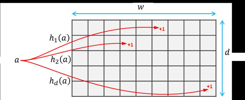
The sequential algorithm’s underlying data structure is a matrix c of w × d counters, for
some parameters w, d determined accordingly to the desired error and probability bounds.
The sketch uses d hash functions hi : Σ 7→ [1, w], for 1 ≤ i ≤ d. The hash functions are
generated using the random coin flip vector #» c , and have certain mathematical properties
whose details are not essential for understanding this paper. The algorithm’s input (i.e., the
schedule) is generated by a so-called weak adversary, namely, the input is independent of the
randomly drawn hash functions.
The CountMin sketch, denoted CM ( #» c ), is illustrated in Figure 1, and its pseudo-code is
given in Algorithm 1. On update(a), the sketch increments counters c[i][hi (a)] for every
1 ≤ i ≤ d. query(a) returns fˆa = min1≤i≤d {c[i][hi (a)]}.
Algorithm 1 CountMin( #»
c ) sketch.
1: array c[1 . . . d][1 . . . w] . Initialized to 0
2: hash functions h1 , . . . hd . hi : Σ 7→ [1, w], initialized using #»
c
3: procedure update(a)
4: for i : 1 ≤ i ≤ d do
5: atomically increment c[i][hi (a)]
6: procedure query(a)
7: min ← ∞
8: for i : 1 ≤ i ≤ d do
9: c ← c[i][hi (a)]
10: if min > c then min ← c
11: return min
Cormode et al. show that, for desired bounds δ and α, given appropriate values of w
and d, with probability at least 1 − δ, the estimate of a query returning fˆa is bounded by
fa ≤ fˆa ≤ fa + αn, where n is the the number of updates preceding the query and fa is
the ideal value. Thus, for = αn, CM is a sequential (, δ)-bounded object. Its sequential
specification distribution is {CM ( #»
c )} #»
c ∈Ω∞ .
Proving an error bound for an efficient parallel implementation of the CM sketch for
existing criteria is not trivial. Using the framework defined by Rinberg et al. [32] requires
the query to take a strongly linearizable snapshot of the matrix [29]. Distributional linear-
izability [2] necessitates an analysis of the error bounds directly in the concurrent setting,
without leveraging the sketch’s existing analysis for the sequential setting.
Instead, we utilize IVL to leverage the sequential analysis for a parallelization that is
not strongly linearizable (or indeed linearizable), without using a snapshot. Consider the
straightforward parallelization of the CM sketch, whereby the operations of Algorithm 1 may
be invoked concurrently and each counter is atomically incremented on line 5 and read on
line 9. We call this parallelization P CM ( #»c ). We next prove that i is IVL.
I Lemma 7. P CM is an IVL implementation of CM .
Proof. Let H be a history of an execution σ of P CM . Let H1 be a linearization of H ? such
that every query is linearized prior to every concurrent update, and let H2 be a linearization
of H ? such that every query is linearized after every concurrent update. Let σi for i = 1, 2
be a sequential execution of CM with history Hi . Consider some Q =query(a) that returns
in H, and let U1 , . . . , Uk be the concurrent updates to Q.A. Rinberg and I. Keidar 2:11
Figure 1 An example CountMin sketch, of size w ×d, where h1 (a) = 6, h2 (a) = 4 and hd (a) = w.2
Denote by cσ (Q)[i] the value read by Q from c[i][hi (a)] in line 9 of Algorithm 1 in an
execution σ. As processes only increment counters, for every 1 ≤ i ≤ d, cσ (Q)[i] is at least
cσ1 (Q)[i] (the value when the query starts) and at most cσ2 (Q)[i] (the value when all updates
concurrent to the query complete). Therefore, cσ1 (Q)[i] ≤ cσ (Q)[i] ≤ cσ2 (Q)[i].
Consider a randomly sampled coin flip vector #» c ∈ Ω∞ . Let j be the loop index the
last time query Q alters the value of its local variable min (line 10), i.e., the index of the
minimum read value. As a query in a history of CM ( #» c ) returns the minimum value in
the array, ret(Q, τCM ( c ) (H1 )) ≤ cσ1 (Q)[j]. Furthermore, ret(Q, τCM ( #»
#» c ) (H2 )) is at least
cσ (Q)[j], otherwise Q would have read this value and returned it instead. Therefore:
ret(Q, τCM ( #» #»
c )) (H1 )) ≤ ret(Q, H(P CM, σ, c )) ≤ ret(Q, τCM ( #»
c ) (H2 ))
As needed. J
Combining Lemma 7 and Theorem 6, and by utilizing the sequential error analysis
from [7], we have shown the following corollary:
I Corollary 8. Let fˆa be a return value from query Q. Let fastart be the ideal frequency of
element a when the query starts, and let faend be the ideal frequency of element a at its end,
and let = αn where n is the stream length at the end of the query. Then:
fastart ≤ fˆa ≤ faend + with probability at least 1 − δ.
The following example demonstrates that P CM is not a linearizable implementation of
CM .
I Example 9. Consider the following execution σ of P DC: Assume that #»
c is such that
h1 (a) = h2 (a) = 1, h1 (b) = 2 and h2 (b) = 1. Assume that initially
1 4
c= .
2 3
First, process p invokes U =update(a) which increments c[1][1] to 2 and stalls. Then,
process p invokes Q1 =query(a) which reads c[1][1] and c[2][1] and returns 2, followed by
Q2 =query(b) which reads c[1][2] and c[2][1] and returns 2. Finally, process p increments
c[2][1] to be 3.
Assume by contradiction that H is a linearization if σ, and H ∈ CM ( #»
c ). The return
values imply that U ≺H Q1 and Q2 ≺H U . As H is a linearization, it maintains the partial
order of operations in σ, therefore Q1 ≺H Q2 . A contradiction.
2
Source: https://stackoverflow.com/questions/6811351/explaining-the-count-sketch-algorithm,
with alterations.
DISC 20202:12 Intermediate Value Linearizability
6 Shared batched counter
We now show an example where IVL is inherently less costly than linearizability. In Section 6.1
we present an IVL batched counter, and show that the update operation has step complexity
O(1). The algorithm uses single-writer-multi-reader(SWMR) registers. In Section 6.2 we
prove that all linearizable implementations of a batched counter using SWMR registers
have step complexity Ω(n) for the update operation. This is in contrast with standard
(non-batched) counters, which can be implemented with a constant update time. Intuitively,
the difference is that in a standard counter, all intermediate values “occur” in an execution
(provided that return values are all integers and increments all add one), and so all values
allowed by IVL are also allowed by linearizability.
6.1 IVL batched counter
We consider a batched counter object, which supports the operations update(v) where v ≥ 0,
and read(). The sequential specification for this object is simple: a read operation returns
the sum of all values passed to update operations that precede it, and 0 if no update
operations were invoked. The update operation returns nothing. When the object is shared,
we denote an invocation of update by process i as updatei . We denote the sequential
specification of the batched counter by H.
Algorithm 2 Algorithm for process pi , implementing an IVL batched counter.
1: shared array v[1 . . . n]
2: procedure updatei (v)
3: v[i] ← v[i] + v
4: procedure read
5: sum ← 0
6: for i : 1 ≤ i ≤ n do
7: sum ← sum + v[i]
8: return sum
Algorithm 2 presents an IVL implementation for a batched counter with n processes
using an array v of n SWMR registers. The implementation is a trivial parallelization: an
update operation increments the process’s local register while a read scans all registers
and returns their sum. This implementation is not linearizable because the reader may see a
later update and miss an earlier one, as illustrated in Figure 2. We now prove the following
lemma:
I Lemma 10. Algorithm 2 is an IVL implementation of a batched counter.
Proof. Let H be a well-formed history of an execution σ of Algorithm 2. We first complete
H be adding appropriate responses to all update operations, and removing all pending
read operations, we denote this completed history as H 0 .
Let H1 be a linearization of H 0? given by ordering update operations by their return steps,
and ordering read operations after all preceding operations in H 0? , and before concurrent
ones. Operations with the same order are ordered arbitrarily. Let H2 be a linearization
of H 0? given by ordering update operations by their invocations, and ordering read
operations operations before all operations that precede them in H 0? , and after concurrent
ones. Operations with the same order are ordered arbitrarily. Let σi for i = 1, 2 be a
sequential execution of a batched counter with history τH (Hi ).A. Rinberg and I. Keidar 2:13
By construction, H1 and H2 are linearizations of H 0? . Let R be some read operation that
completes in H. Let v[1 . . . n] be the array as read by R in σ, v1 [1 . . . n] as read by R in σ1 and
v2 [1 . . . n] as read by R in σ2 . To show that ret(R, τH (H1 )) ≤ ret(R, H) ≤ ret(R, τH (H2 )),
we show that v1 [j] ≤ v[j] ≤ v2 [j] for every index 1 ≤ j ≤ n.
For some index j, only pj can increment v[j]. By the construction of H1 , all update
operations that precede R in H also precede it in H1 . Therefore v1 [j] ≤ v[j]. Assume by
contradiction that v[j] > v2 [j]. Consider all concurrent update operations to R. After all
concurrent update operations end, the value of index j is v 0 ≥ v[j] > v2 [j]. However, by
construction, R is ordered after all concurrent update operations in H2 , therefore v 0 ≤ v2 [j].
This is a contradiction, and therefore v[j] ≤ v2 [j].
Pn Pn
As all entries in the array are non-negative, it follows that j=1 v1 [j] ≤ j=1 v[j] ≤
Pn
j=1 v2 [j], and therefore ret(R, τH (H1 )) ≤ ret(R, H) ≤ ret(R, τH (H2 )). J
Figure 2 shows a possible concurrent execution of Algorithm 2. This algorithm can
efficiently implement a distributed or NUMA-friendly counter, as processes only access
their local registers thereby lowering the cost of incrementing the counter. This is of great
importance, as memory latencies are often the main bottleneck in shared object emulations [25].
As there are no waits in either update or read, it follows that the algorithm is wait-free.
Furthermore, the read step complexity is O(n), and the update step complexity is O(1).
Thus, we have shown the following theorem:
I Theorem 11. There exists a bounded wait-free IVL implementation of a batched counter
using only SWMR registers, such that the step complexity of update is O(1) and the step
complexity of read is O(n).
6.2 Lower bound for linearizable batched counter object
The incentive for using an IVL batched counter instead of a linearizable one stems from a
lower bound on the step-complexity of a wait-free linearizable batched counter implementation
from SWMR registers. To show the lower bound we first define the binary snapshot object.
A snapshot object has n components written by separate processes, and allows a reader
to capture the shared variable states of all n processes instantaneously. We consider the
binary snapshot object, in which each state component may be either 0 or 1 [20]. The object
supports the updatei (v) and scan operations, where the former sets the state of component
i to value a v ∈ {0, 1} and the latter returns all processes states instantaneously. It is trivial
that the scan operation must read all states, therefore its lower bound step complexity is
Ω(n). Israeli and Shriazi [21] show that the update step complexity of any implementation
of a snapshot object from SWMR registers is also Ω(n). This lower bound was shown to hold
also for multi writer registers [3]. While their proof was originally given for a multi value
snapshot object, it holds in the binary case as well [20].
Figure 2 A possible concurrent history of the IVL batched counter: p1 and p2 update their local
registers, while p3 reads. p3 returns an intermediate value between the counter’s state when it starts,
which is 0, and the counter’s state when it completes, which is 10.
DISC 20202:14 Intermediate Value Linearizability
Algorithm 3 Algorithm for process pi , solving binary snapshot with a batched counter object.
1: local variable vi . Initialized to 0
2: shared batched counter object BC
3: procedure updatei (v)
4: if vi = v then return
5: vi ←v
6: if v = 1 then BC .updatei (2i )
7: if v = 0 then BC .updatei (2n − 2i )
8: procedure scan
9: sum ← BC .read()
10: v[0 . . . n − 1] ← [0 . . . 0] . Initialize an array of 0’s
11: for i : 0 ≤ i ≤ n − 1 do
12: if bit i is set in sum then v[i] ← 1
13: return v[0 . . . n − 1]
To show a lower bound on the update operation of wait-free linearizable batched counters,
we show a reduction from a binary snapshot to a batched counter in Algorithm 3. It uses a
local variable vi and a shared batched counter object. In a nutshell, the idea is to encode the
value of the ith component of the binary snapshot using the ith least significant bit of the
counter. When the component changes from 0 to 1, updatei adds 2i , and when it changes
from 1 to 0, updatei adds 2n − 2i . We now prove the following invariant:
I Invariant 1. At any point t in history H of a sequential execution of Algorithm 3, the
Pn−1
sum held by the counter is c · 2n + i=0 vi 2i , such that vi is the parameter passed to the last
invocation of updatei in H 0 before t if such invocation exists, and 0 otherwise, for some
integer c ∈ N.
Proof. We prove the invariant by induction on the length of H, i.e., the number of invocations
in H, denoted t. As H is a sequential history, each invocation is followed by a response.
Base: The base if for t = 0, i.e., H is the empty execution. In this case no updates have
been invoked, therefore vi = 0 for all 0 ≤ i ≤ n − 1. The sum returned by the counter is 0.
Choosing c = 0 satisfies the invariant.
Induction step: Our induction hypothesis is that the invariant holds for a history
of length t. We prove that it holds for a history of length t + 1. The last invocation
can be either a scan, or an update(v) by some process pi . If it is a scan, then the
counter value doesn’t change and the invariant holds. Otherwise, it is an update(v). Here,
we note two cases. Let vi be pi ’s value prior to the update(v) invocation. If v = vi ,
then the update returns without altering the sum and the invariant holds. Otherwise,
v =6 vi . We analyze two cases, v = 1 and v = 0. If v = 1, then vi = 0. The sum after
Pn−1 Pn−1
the update is c · 2n + i=0 vi 2i + 2i = c · 2n + i=0 vi0 2i , where vj0 = vj if j = 6 i, and
vi0 = 1, and the invariant holds. If v = 0, then vi = 1. The sum after the update is
Pn−1 Pn−1
c · 2n + i=0 vi 2i + 2n − 2i = (c + 1) · 2n + i=0 vi0 2i , where vj0 = vj if j 6= i, and vi0 = 1,
and the invariant holds. J
Using the invariant, we prove the following lemma:
I Lemma 12. For any sequential history H, if a scan returns vi , and updatei (v) is the
last update invocation in H prior to the scan, then vi = v. If no such update exists, then
vi = 0.A. Rinberg and I. Keidar 2:15
Proof. Let S be a scan in H 0 . Consider the sum sum as read by scan S. From Invariant 1,
Pn−1
the value held by the counter is c · 2n + i=0 vi 2i . There are two cases, either there is
an update invocation prior to S, or there isn’t. If there isn’t, then by Invariant 1 the
corresponding vi = 0. The process sees bit i = 0, and will return 0. Therefore, the lemma
holds.
Pn−1
Otherwise, there is a an update prior to S in H. As the sum is equal to c · 2n + i=0 vi 2i ,
by Invariant 1, bit i is equal to 1 iff the parameter passed to the last invocation of update was
1. Therefore, the scan returns the parameter of the last update and the lemma holds. J
I Lemma 13. Algorithm 3 implements a linearizable binary snapshot using a linearizable
batched counter.
Proof. Let H be a history of Algorithm 3, and let H 0 be H where each operation is linearized
at its access to the linearizable batched counter, or its response if vi = v on line 4. Applying
Lemma 12 to H 0 , we get H 0 ∈ H and therefore H is linearizable. J
It follows from the algorithm that if the counter object is bounded wait-free then the
scan and update operations are bounded wait-free. Therefore, the lower bound proved by
Israeli and Shriazi [21] holds, and the update must take Ω(n) steps. Other than the access
to the counter in the update operation, it takes O(1) steps. Therefore, the access to the
counter object must take Ω(n) steps. We have proven the following theorem.
I Theorem 14. For any linearizable wait-free implementation of a batched counter object
with n processes from SWMR registers, the step-complexity of the update operation is Ω(n).
7 Conclusion
We have presented IVL, a new correctness criterion that provides flexibility in the return
values of quantitative objects while bounding the error that this may introduce. IVL has
a number of desirable properties: First, like linearizability, it is a local property, allowing
designers to reason about each part of the system separately. Second, also like linearizability
but unlike other relaxations of it, IVL preserves the error bounds of PAC objects. Third,
IVL is generically defined for all quantitative objects, and does not necessitate object-
specific definitions. Finally, IVL is inherently amenable to cheaper implementations than
linearizability in some cases.
Via the example of a CountMin sketch, we have illustrated that IVL provides a generic
way to efficiently parallelize data sketches while leveraging their sequential error analysis to
bound the error in the concurrent implementation.
The notion of IVL raises a number of questions for future research. First, in this work we
have shown that IVL is a sufficient condition for parallel (, δ)-bounded objects, in that it
preserves their sequential error. It would be interesting to investigate whether IVL is also
necessary, or whether some weaker condition is sufficient. Second, we would like to extend
IVL to objects like priority queues, which are in a sense “semi quantitative”, namely, their
return values are associated with a quantity (the priority) but also include a non-quantitative
element (the queued item). Additionally, it could be useful to apply IVL to additional
sketches, and to study whether it can meaningfully apply to non-monotonic quantities.
DISC 20202:16 Intermediate Value Linearizability
References
1 Pankaj K Agarwal, Graham Cormode, Zengfeng Huang, Jeff M Phillips, Zhewei Wei, and
Ke Yi. Mergeable summaries. ACM Transactions on Database Systems (TODS), 38(4):1–28,
2013.
2 Dan Alistarh, Trevor Brown, Justin Kopinsky, Jerry Z Li, and Giorgi Nadiradze. Distribution-
ally linearizable data structures. In Proceedings of the 30th on Symposium on Parallelism in
Algorithms and Architectures, pages 133–142. ACM, 2018.
3 Hagit Attiya, Faith Ellen, and Panagiota Fatourou. The complexity of updating multi-writer
snapshot objects. In International Conference on Distributed Computing and Networking,
pages 319–330. Springer, 2006.
4 Armando Castañeda, Sergio Rajsbaum, and Michel Raynal. Unifying concurrent objects and
distributed tasks: Interval-linearizability. Journal of the ACM (JACM), 65(6):1–42, 2018.
5 Jacek Cichon and Wojciech Macyna. Approximate counters for flash memory. In 2011
IEEE 17th International Conference on Embedded and Real-Time Computing Systems and
Applications, volume 1, pages 185–189. IEEE, 2011.
6 Graham Cormode, Minos Garofalakis, Peter J Haas, and Chris Jermaine. Synopses for
massive data: Samples, histograms, wavelets, sketches. Foundations and Trends in Databases,
4(1–3):1–294, 2012.
7 Graham Cormode and Shan Muthukrishnan. An improved data stream summary: the
count-min sketch and its applications. Journal of Algorithms, 55(1):58–75, 2005.
8 Graham Cormode, Shanmugavelayutham Muthukrishnan, and Ke Yi. Algorithms for distrib-
uted functional monitoring. ACM Transactions on Algorithms (TALG), 7(2):1–20, 2011.
9 Mayur Datar and Piotr Indyk. Comparing data streams using hamming norms. In Proceedings
2002 VLDB Conference: 28th International Conference on Very Large Databases (VLDB),
page 335. Elsevier, 2002.
10 Druid. Apache DataSketches (Incubating). https://incubator.apache.org/clutch/
datasketches.html, Accessed May 14, 2020.
11 Druid. Druid. https://druid.apache.org/blog/2014/02/18/
hyperloglog-optimizations-for-real-world-systems.html, Accessed May 14, 2020.
12 Philippe Flajolet. Approximate counting: a detailed analysis. BIT Numerical Mathematics,
25(1):113–134, 1985.
13 Philippe Flajolet and G Nigel Martin. Probabilistic counting. In 24th Annual Symposium on
Foundations of Computer Science (sfcs 1983), pages 76–82. IEEE, 1983.
14 Phillip B Gibbons and Srikanta Tirthapura. Estimating simple functions on the union of data
streams. In Proceedings of the thirteenth annual ACM symposium on Parallel algorithms and
architectures, pages 281–291, 2001.
15 Wojciech Golab, Lisa Higham, and Philipp Woelfel. Linearizable implementations do not
suffice for randomized distributed computation. In Proceedings of the forty-third annual ACM
symposium on Theory of computing, pages 373–382, 2011.
16 Thomas A Henzinger, Christoph M Kirsch, Hannes Payer, Ali Sezgin, and Ana Sokolova.
Quantitative relaxation of concurrent data structures. In Proceedings of the 40th annual ACM
SIGPLAN-SIGACT symposium on Principles of programming languages, pages 317–328, 2013.
17 Maurice P Herlihy and Jeannette M Wing. Linearizability: A correctness condition for
concurrent objects. ACM Transactions on Programming Languages and Systems (TOPLAS),
12(3):463–492, 1990.
18 Stefan Heule, Marc Nunkesser, and Alexander Hall. Hyperloglog in practice: algorithmic
engineering of a state of the art cardinality estimation algorithm. In Proceedings of the 16th
International Conference on Extending Database Technology, pages 683–692, 2013.
19 Hillview. Hillview: A Big Data Spreadsheet. https://research.vmware.com/projects/
hillview, Accessed May 14, 2020.
20 Jaap-Henk Hoepman and John Tromp. Binary snapshots. In International Workshop on
Distributed Algorithms, pages 18–25. Springer, 1993.A. Rinberg and I. Keidar 2:17
21 Amos Israeli and Asaf Shirazi. The time complexity of updating snapshot memories. Informa-
tion Processing Letters, 65(1):33–40, 1998.
22 Leslie Lamport. On interprocess communication. Distributed computing, 1(2):86–101, 1986.
23 Leslie Lamport. Concurrent reading and writing of clocks. ACM Transactions on Computer
Systems (TOCS), 8(4):305–310, 1990.
24 Zaoxing Liu, Antonis Manousis, Gregory Vorsanger, Vyas Sekar, and Vladimir Braverman.
One sketch to rule them all: Rethinking network flow monitoring with univmon. In Proceedings
of the 2016 ACM SIGCOMM Conference, pages 101–114, 2016.
25 Nihar R Mahapatra and Balakrishna Venkatrao. The processor-memory bottleneck: problems
and solutions. XRDS: Crossroads, The ACM Magazine for Students, 5(3es):2, 1999.
26 Ahmed Metwally, Divyakant Agrawal, and Amr El Abbadi. Efficient computation of frequent
and top-k elements in data streams. In International Conference on Database Theory, pages
398–412. Springer, 2005.
27 Robert Morris. Counting large numbers of events in small registers. Communications of the
ACM, 21(10):840–842, 1978.
28 Gil Neiger. Set-linearizability. In Proceedings of the thirteenth annual ACM symposium on
Principles of distributed computing, page 396, 1994.
29 Sean Ovens and Philipp Woelfel. Strongly linearizable implementations of snapshots and other
types. In Proceedings of the 2019 ACM Symposium on Principles of Distributed Computing,
pages 197–206, 2019.
30 Presto. HyperLogLog in Presto: A significantly faster way to handle cardinality estima-
tion. https://engineering.fb.com/data-infrastructure/hyperloglog/, Accessed May 14,
2020.
31 Arik Rinberg and Idit Keidar. Intermediate value linearizability: A quantitative correctness
criterion. arXiv preprint arXiv:2006.12889, 2020.
32 Arik Rinberg, Alexander Spiegelman, Edward Bortnikov, Eshcar Hillel, Idit Keidar, Lee
Rhodes, and Hadar Serviansky. Fast concurrent data sketches. In Proceedings of the 2020
ACM Symposium on Principles and Practice of Parallel Programming. ACM, 2020.
33 Charalampos Stylianopoulos, Ivan Walulya, Magnus Almgren, Olaf Landsiedel, and Marina
Papatriantafilou. Delegation sketch: a parallel design with support for fast and accurate
concurrent operations. In Proceedings of the Fifteenth European Conference on Computer
Systems, pages 1–16, 2020.
DISC 2020You can also read