Using Satellite Error Modeling to Improve GPM-Level 3 Rainfall Estimates over the Central Amazon Region - MDPI
←
→
Page content transcription
If your browser does not render page correctly, please read the page content below
remote sensing
Article
Using Satellite Error Modeling to Improve
GPM-Level 3 Rainfall Estimates over the Central
Amazon Region
Rômulo Oliveira 1,2, *,†      ID
                                   , Viviana Maggioni 2   ID
                                                               , Daniel Vila 1   ID
                                                                                      and Leonardo Porcacchia 2
 1   Centro de Previsão de Tempo e Estudos Climáticos (CPTEC), Instituto Nacional de Pesquisas
     Espaciais (INPE), São José dos Campos, SP 12227-010, Brazil; daniel.vila@inpe.br
 2   Sid and Reva Dewberry Department of Civil, Environmental, and Infrastructure Engineering, George Mason
     University, Fairfax, VA 22030, USA; vmaggion@gmu.edu (V.M.); lporcacc@masonlive.gmu.edu (L.P.)
 *   Correspondence: romulo.augusto@cptec.inpe.br; Tel.: +55-12-3208-6821
 †   Current address: Géosciences Environnement Toulouse (GET), Centre National de la Recherche Scientifique,
     Toulouse 31055, France.

 Received: 29 December 2017; Accepted: 21 February 2018; Published: 23 February 2018

 Abstract: This study aims to assess the characteristics and uncertainty of Integrated Multisatellite
 Retrievals for Global Precipitation Measurement (GPM) (IMERG) Level 3 rainfall estimates and to
 improve those estimates using an error model over the central Amazon region. The S-band Amazon
 Protection National System (SIPAM) radar is used as reference and the Precipitation Uncertainties
 for Satellite Hydrology (PUSH) framework is adopted to characterize uncertainties associated with
 the satellite precipitation product. PUSH is calibrated and validated for the study region and takes
 into account factors like seasonality and surface type (i.e., land and river). Results demonstrated that
 the PUSH model is suitable for characterizing errors in the IMERG algorithm when compared with
 S-band SIPAM radar estimates. PUSH could efficiently predict the satellite rainfall error distribution
 in terms of spatial and intensity distribution. However, an underestimation (overestimation) of light
 satellite rain rates was observed during the dry (wet) period, mainly over rivers. Although the
 estimated error showed a lower standard deviation than the observed error, the correlation between
 satellite and radar rainfall was high and the systematic error was well captured along the Negro,
 Solimões, and Amazon rivers, especially during the wet season.

 Keywords: global precipitation measurement; IMERG; PUSH; error model; validation; Amazon

1. Introduction
      Satellite rainfall estimates have been widely used across Brazil for various purposes,
e.g., monitoring natural disasters, hydrological modeling, and climate studies [1–3]. Although the
quality of satellite rainfall products has improved significantly in recent decades, such algorithms
require careful validation, which provides information about their performance, limitations, and
associated uncertainties. Understanding and quantifying errors is also extremely important for
algorithm developers to improve the final precipitation products.
      Uncertainties in satellite rainfall estimates arise from different factors, including sensor calibration,
retrieval errors, and spatial and temporal sampling, among others [4,5]. However, the definition and
quantification of uncertainty are directly and indirectly based on the error model definition [6]. Two
types of error models are commonly used for assessing uncertainty in precipitation measurements
(satellite and radar estimates): additive and multiplicative error models. According to Tian et al. [6],
the multiplicative error model is a better choice as it separates the systematic and random errors, can

Remote Sens. 2018, 10, 336; doi:10.3390/rs10020336                                    www.mdpi.com/journal/remotesensing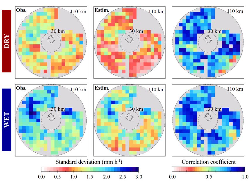
Remote Sens. 2018, 10, 336                                                                          2 of 12

be applied to a wide range of variability in daily precipitation, and produces superior predictions of
the error characteristics.
     To understand the nature of the error in satellite precipitation products, a technique to decompose
the total error into hit, miss-rain, and false-rain biases [7] is considered. Maggioni et al. [8] proposed
the Precipitation Uncertainties for Satellite Hydrology (PUSH) error model framework in order to
provide an estimate of the error associated with high-resolution satellite precipitation products for
each grid point and at each time step. The probability density function (PDF) of the actual rainfall is
modeled differently for missed precipitation cases, false alarms, and hit biases. In the PUSH approach,
the error is considered as a combination of random and systematic components and the hit error is
modeled with a multiplicative error model [9].
     This study aims to assess the characteristics and uncertainty distribution of the Integrated
Multisatellite Retrievals for Global Precipitation Measurement (GPM) (IMERG) rainfall estimates
over the central Amazon region using the S-band Amazon Protection National System (SIPAM) radar
as reference and PUSH as error model. PUSH is calibrated and validated for the study region and takes
into account local factors such as seasonality and surface type (i.e., land and river). This work seeks to
answer the following scientific questions: (i) What are the characteristics and uncertainty distribution
of GPM satellite Level 3 rainfall estimates over the Brazilian Amazon? (ii) How can those uncertainties
be minimized to improve satellite precipitation products for use in hydrological applications over the
region? In Section 2, the study area, precipitation regime, datasets, and methodology are described.
Results of the model calibration and its performance over the study region are presented in Section 3
and discussed in Section 4. Section 5 presents our conclusions and future directions.

2. Study Area, Data, and Methodology
      This work focuses on a region located in the middle of the Amazon basin, around the city of
Manaus in the state of Amazonas, Brazil. The area covers a radius of 110 km centered at 3.15◦ S
and 59.99◦ W, where the operational S-band weather radar from the Amazon Protection National
System (SIPAM) is located (Figure 1). The characteristics and diurnal cycle of precipitation over the
Manaus region have been previously investigated using the S-band SIPAM radar by Oliveira et al. [10],
Burleyson et al. [11], Giagrande et al. [12], and Tang et al. [13]. Oliveira et al. [10] suggested that
the diurnal cycle of precipitation is strongly modulated by weather systems that produce moderate
and heavy rainfall and the rainfall’s volume and occurrence, which depend on the season. However,
according to Burleyson et al. [11], precipitation varies spatially with a preferred location of maximum
rain rate observed east of the Negro River (during the rainy season, from March to May in 2014–2015),
driven by the local and large-scale vertical pattern (updrafts and downdrafts) and thermodynamic
factors (e.g., diabatic heating) of convective rain cells [12,13].
      Oliveira et al. [10] assessed the performance of IMERG in representing the characteristics and
diurnal cycle of precipitation over the study region. During the wet (dry) period, the volume and
occurrence contributions of moderate (heavy) rainfall are clearly identified and strongly modulated by
the precipitation diurnal cycle. A strong dependence of the IMERG dataset performance on seasonality
is also observed. This behavior is prominent over the inland water surface type (along the Negro,
Solimões, and Amazon rivers) due to the poor calibration of the 2014 Goddard Profiling (GPROF)
algorithm (i.e., GMI retrievals) for the continent-ocean surface type.
      The precipitation data used for this study are:

i.       One National Institute of Meteorology (INMET) rain gauge located in Manaus city (at 3.1◦ S
         and 60.0◦ W). The INMET rain gauge is an automatic station that provides hourly records. This
         study uses a period of 30 years of daily accumulations (mm·day−1 );
ii.      The S-band SIPAM radar rainfall estimates, processed by Texas A&M University. The rainfall
         estimates were obtained through the Constant Altitude Plan Position Indicator (CAPPI) product
         at a 2.5 km vertical level. The radial data were initially gridded to a Cartesian grid with 2 km
         × 2 km × 0.5 km resolution every 12 min. However, to match the satellite product, the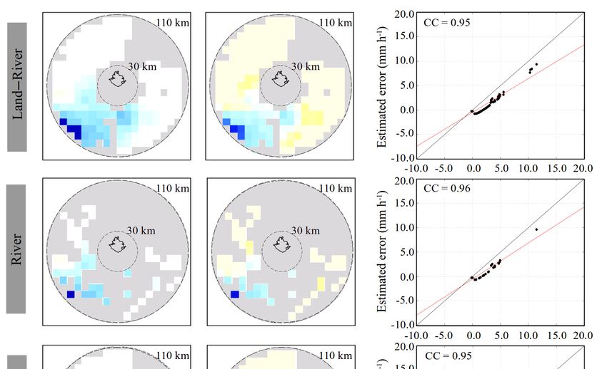
Remote Sens. 2018, 10, 336 3 of 12
radar rainfall retrievals were integrated to 30 min and averaged to 0.1 degrees. To reduce the
uncertainties of the radar rainfall retrievals, the following criteria were adopted: (i) a radar
coverage area of 30–110 km in radius was adopted because of radar physical limitations in
Remote Sens. 2018, 10, x FOR PEER REVIEW 3 of 13
detecting signals directly above it (“cone of silence”) and far at the constant altitude of 2.5 km;
(ii) the areas whereofthe
uncertainties the radar beam was
radar rainfall blocked
retrievals, by nearby
the following objects
criteria werewere masked
adopted: out. We refer
(i) a radar
the reader to Oliveira et al. [10] for a more detailed description of the S-band SIPAMinradar and
coverage area of 30–110 km in radius was adopted because of radar physical limitations
detecting signals directly above it (“cone of silence”) and far at the constant altitude of 2.5 km;
IMERG(ii) rainfall retrievals and their performance over the study region;
the areas where the radar beam was blocked by nearby objects were masked out. We refer
iii. The Integrated
the reader Multisatellite Retrievals
to Oliveira et al. [10] for a morefor GPMdescription
detailed (IMERG)—GPM
of the S-band Level
SIPAM 3 rainfall
radar andestimates
(V03D, IMERG
Final run rainfall retrievals
version). andIMERG
The their performance
Final run over product is a quasi-global (60◦ N–S)
the study region;
(research)
iii. The Integrated Multisatellite Retrievals for GPM (IMERG)—GPM Level 3 rainfall estimates
dataset, with 0.1◦ /30 min spatial/temporal resolution and currently available for March
(V03D, Final run version). The IMERG Final run (research) product is a quasi-global (60° N–S)
2014–present [14,15]. Although newer versions
dataset, with 0.1°/30 min spatial/temporal of this product
resolution haveavailable
and currently and willforbecome
March available,
the methodology
2014–present [14,15]. Although newer versions of this product have and will become available,of IMERG.
developed in this work can be easily adapted to any future version
the methodology
By choosing the Finaldeveloped
run, which in this work canabemonthly
includes easily adapted to any
gauge future version
adjustment, weof present
IMERG. here the
By choosing the Final run, which includes a monthly gauge adjustment, we present here the
best-case scenario in terms of errors associated with the IMERG product and the worst-case
best-case scenario in terms of errors associated with the IMERG product and the worst-case
scenarioscenario
in terms of error
in terms correction
of error correctionwith PUSH.InIn
with PUSH. other
other words,
words, the correction
the correction scheme would
scheme would
have more have room
more room for improvement
for improvementand lookmore
and look more impressive
impressive if applied
if applied to the
to the Late Late or Early
or Early
near-real-time
near-real-time runs,runs, which
which lackthe
lack the bias
bias adjustment.
adjustment.
Figure 1. Study
Figurearea; S-band
1. Study Amazon
area; S-band Protection
Amazon ProtectionNational System
National System (SIPAM)
(SIPAM) radarradar
locationlocation in Manaus
in Manaus
(in red), Amazonas
(in red), Amazonas (AM); and(AM);surface
and surface class
class masks(land
masks (land and
andriver, land
river, only,
land and river
only, and only).
river only).
The study period is 12 March 2014 to 17 August 2015 (17 months of half-hourly resolution
The study period
coincident is 12 March
radar–satellite 2014 toThis
observations). 17 August 2015the(17
period covers twomonths
Intensiveof half-hourly
Operating Periodsresolution
(IOPs) of the last Cloud processes of tHe main precipitation systems
coincident radar–satellite observations). This period covers the two Intensive Operating in Brazil: A contribUtion to Periods
cloud resolVing modeling and to the GlobAl Precipitation Measurement (CHUVA) [16] and the
(IOPs) of the last Cloud processes of tHe main precipitation systems in Brazil: A contribUtion to
Observations and Modeling of the Green Ocean Amazon (GoAmazon) [17] campaigns, held in
cloud resolVing
Manaus modeling
city during the andwetto the GlobAl
season, Precipitation
from 1 February to 31 March Measurement
2014 (IOP1), and(CHUVA)
dry season, from [16] and the
Observations and Modeling
15 August to 15 Octoberof the
2014Green
(IOP2). Ocean Amazon
According to Martin (GoAmazon) [17]rainfall
et al. [17], the 2014 campaigns, held in Manaus
regime showed
city duringpositive
the wet precipitation
season, from anomalies (~200 mm)
1 February to during
31 Marchthe wet
2014period over the
(IOP1), andAmazon region. from
dry season, During15 August
the dry period, the positive and negative anomalies of rainfall amounts were spatially distributed
to 15 October 2014 (IOP2). According to Martin et al. [17], the 2014 rainfall regime showed positive
over the region. In addition, regarding the 2014/15 rainfall regime over the central Amazon region,
precipitation anomalies
Marengo (~200
et al. [18] mm)
found during
a delay the2014/15
in the wet period
onset toover the 2015,
January Amazon whichregion.
resulted During
in the
dry period,below-normal
the positive and negative
precipitation. anomalies ofcontext
The meteorological rainfall amounts
related were spatially
to the onset/demise distributed
of the 2014/5 over
the region.rainy
In season over the
addition, Manaus region
regarding was strongly
the 2014/15 relatedregime
rainfall to dynamicoverfactors—for
the central example,
Amazon the region,
Madden–Julian Oscillation (MJO) effect—and was less influenced by thermodynamic factors [18].
Marengo et al. [18] found a delay in the 2014/15 onset to January 2015, which resulted in below-normal
Uncertainties associated with the IMERG rainfall estimates over the central Amazon region
precipitation. The
depend on meteorological
the surface type andcontext relatedregime
the precipitation to the onset/demise
[10]. of the 2014/5
Therefore, it is important rainy season
to investigate
over the Manaus region
and quantify was strongly
the impact related
of these factors to dynamic
on the performance factors—for example,
of satellite retrievals. The the Madden–Julian
surface type
Oscillation (MJO) effect—and was less influenced by thermodynamic factors [18].
Uncertainties associated with the IMERG rainfall estimates over the central Amazon region
depend on the surface type and the precipitation regime [10]. Therefore, it is important to investigate
and quantify the impact of these factors on the performance of satellite retrievals. The surface type
factor consists of a land cover map that discriminates the surface type (in this case, land and inland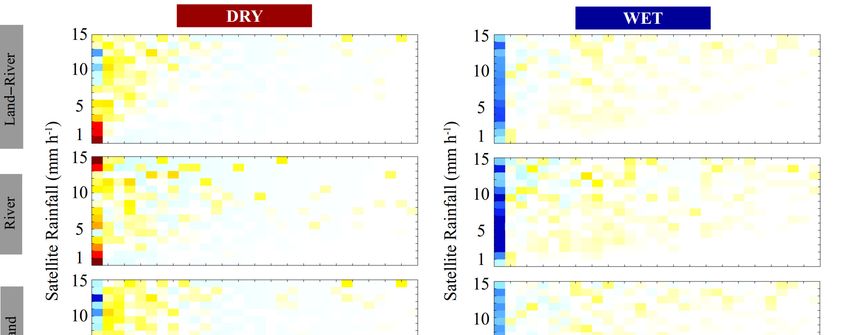
Remote Sens. 2018, 10, 336 4 of 12
water) in the satellite algorithm. Thus, three surface classes (land, river, and land–river) were adopted
and investigated separately.
Figure 1 shows the study area, the S-band SIPAM radar 110 km coverage radius, and the masks of
the three surface classes, which account for the S-band SIPAM radar limitations. The hydrographic
and radar limitation masks are therefore combined and resampled to a 0.1◦ × 0.1◦ grid to match the
IMERG spatial resolution.
The seasonality factor (precipitation regimes) also plays a fundamental role in the Brazilian
Amazon [16–23]. Although the Amazon region presents a very well defined and regionalized dry
and wet season pattern
Remote Sens. 2018,[22],
10, x FORsuch behaviors may vary depending on the year under
PEER REVIEW 4 of 13 investigation
and the interaction of remote and large-scale phenomena [23]. Liebmann and Marengo [19]
factor consists of a land cover map that discriminates the surface type (in this case, land and inland
developed an water)
objective method
in the satellite of onset
algorithm. andsurface
Thus, three demise classesidentification of the rainy
(land, river, and land–river) were season, later
adopted and investigated
adapted by Liebmann et al. [24], separately.
Bombardi and Carvalho et al. [25], and Coelho et al. [26].
Figure 1 shows the study area, the S-band SIPAM radar 110 km coverage radius, and the masks
The Coelho et al. [26]three
of the version
surfaceisclasses,
currentlywhichoperational
account for the at S-band
the Center
SIPAM for radarWeather
limitations.and TheClimate Studies
(CPTEC) (http://clima1.cptec.inpe.br/). The Liebmann and Marengo [19] methodology takes into
hydrographic and radar limitation masks are therefore combined and resampled to a 0.1° × 0.1° grid
to match the IMERG spatial resolution.
account the relation between mean precipitation for the pentad (mm·day−1 ) and climatological annual
The seasonality factor (precipitation regimes) also plays a fundamental role in the Brazilian
mean daily precipitation
Amazon [16–23]. (mm ·day−
Although 1 )Amazon
the to defineregionthe onseta very
presents andwelldemise
definedof andthe rainy season.
regionalized dry
and wet season pattern [22], such behaviors may vary depending on the year under investigation
Thus, IMERG errors are investigated for different surface types
and the interaction of remote and large-scale phenomena [23]. Liebmann and Marengo [19]
(land and inland water) and
seasons (dry and wet). The Liebmann and Marengo [19] criterion is used
developed an objective method of onset and demise identification of the rainy season, later adapted to identify the onset and
by Liebmann et al. [24], Bombardi and Carvalho et al. [25], and Coelho
demise of the rainy and dry seasons in the dataset period. The approach is applied to a single rain et al. [26]. The Coelho et al.
[26] version is currently operational at the Center for Weather and Climate Studies (CPTEC)
gauge station, (http://clima1.cptec.inpe.br/).
located within the radar coverage
The Liebmann area [19]
and Marengo (Manaus
methodologycity).takesBased on the
into account the 17 months of
IMERG and radar data (coincident time steps), four distinct periods were considered. The time series
relation between mean precipitation for the pentad (mm∙day −1) and climatological annual mean
daily precipitation (mm∙day−1) to define the onset and demise of the rainy season.
for calibration andThus,validation
IMERG errors (independent
are investigatedperiod)
for differentare defined
surface for both
types (land the water)
and inland wet and and dry seasons in
Table 1. The wet season
seasons (dry period
and wet).used for calibration
The Liebmann and Marengo is [19]
consistent
criterion iswith
used tothe rainy
identify theseason
onset andcharacterized by
Marengo et al. demise of the rainy and dry seasons in the dataset period. The approach is applied to a single rain
[18]. The wet season designated for validation includes part of the IOP1. The IOP2 is
gauge station, located within the radar coverage area (Manaus city). Based on the 17 months of
completely inserted
IMERG in andthe
radar calibration
data (coincident dry
timeperiod. Figure
steps), four distinct 2 illustrates
periods the precipitation
were considered. The time series regimes during
the wet and dry forperiods.
calibration and validation (independent period) are defined for both the wet and dry seasons in
Table 1. The wet season period used for calibration is consistent with the rainy season characterized
by Marengo et al. [18]. The wet season designated for validation includes part of the IOP1. The IOP2
Table 1. Precipitation
is completely Uncertainties for Satellite
inserted in the calibration Hydrology
dry period. Figure (PUSH) calibration
2 illustrates and validation
the precipitation regimes periods
during the wet and
during the wet and dry seasons.dry periods.
Table 1. Precipitation Uncertainties for Satellite Hydrology (PUSH) calibration and validation
periods during the wet and dry seasons. Periods Time Steps
Dry 15 June 2014–21 December 2014Time Steps
Periods 8043
Calibration
WetDry 22June
15 December
2014–212014–23 May
December 2015 8043
2014 6641
Calibration
DryWet 2224
December 2014–23 May 2015
May 2015–17 August 2015 6641 3416
Validation Dry 24
ValidationWet 12May 2015–17
March August
2014–14 2015
June 2014 3416 3865
Wet 12 March 2014–14 June 2014 3865
Figure 2. Precipitation regime over Manaus city (National Institute of Meteorology (INMET) station)
Figure 2. Precipitation regime
and wet (blue) over
and dry Manaus
(red) cityPUSH
periods for (National Institute
calibration of Meteorology
and validation. The shaded area(INMET) station)
and wet (blue) represents
and drythe rainy periods
(red) season based onPUSH
for the Climatological Normal
calibration (1961–1990)
and shown with
validation. Thea black
shadedline. area represents
the rainy season based on the Climatological Normal (1961–1990) shown with a black line. Wet and
dry periods are based on the Liebmann and Marengo [19] criterion, which takes into account the
actual observations (gray line). The CHUVA/GoAmazon IOP1 (wet) and IOP2 (dry) periods are
also indicated.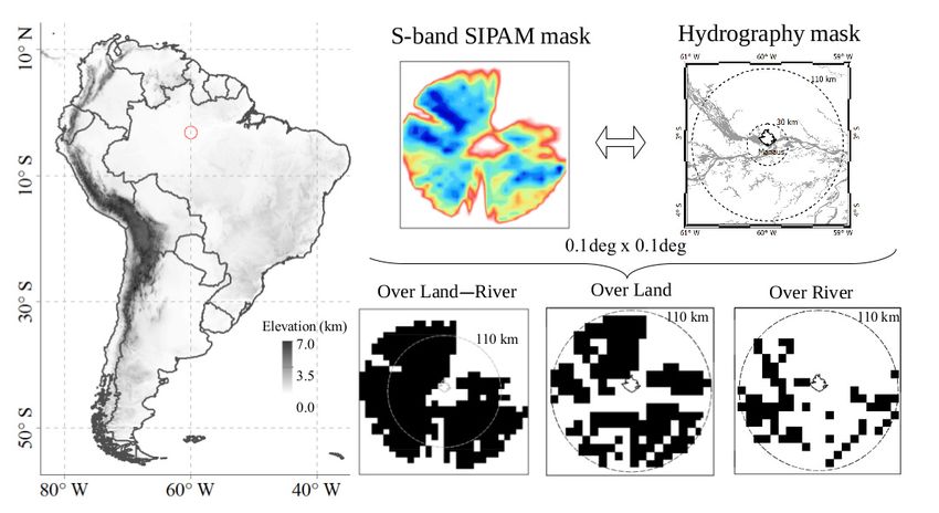
Remote Sens. 2018, 10, 336                                                                              5 of 12

     The PUSH model, recently developed by Maggioni et al. [8], was adopted to characterize errors
associated with IMERG at each grid point and time step. PUSH assesses the probability density
function (PDF) of the actual precipitation by decomposing the satellite precipitation error for the
following cases: (i) correct no-precipitation detection (Case 00); (ii) missed precipitation events (the
satellite records a zero, but the reference detects precipitation, Case 01); (iii) false alarms (the satellite
incorrectly detects precipitation, as the reference observes no rain, Case 10); and (iv) hit biases (both
satellite and reference detect precipitation, but may disagree on the amount, Case 11).
     Given the IMERG satellite observation X and the S-band reference SIPAM radar precipitation
observation Y, the PUSH framework provides an estimate of the PDF of the actual precipitation Y at
30 min and 0.1◦ temporal and spatial resolution. The satellite error can then be computed as either the
difference or the ratio between the satellite X and the expected value of the estimated precipitation
distribution. PUSH was calibrated for IMERG for different surface types (land and inland water)
and seasons (dry and wet) and using a rain/no rain threshold of 0.2 mm·h−1 . Once calibration was
completed, the model performance was validated during an independent period.

3. Results

3.1. Model Calibration
      The PUSH model was calibrated for three separate conditions (over land–river, over river only, and
over land only) during the dry and wet seasons over the central Amazon region. The performance of
PUSH obtained during the calibration step is briefly described here and presented in the Supplementary
Material (Figures S1–S3). The probabilities of correct no-precipitation detection (P00) and missed
precipitation (P01 = 1 − P00) for the over land–river, over river only, and over land only surface type
conditions were computed for both the dry and wet seasons. Such information provides a general
estimate of the probability of false alarms (P10) and hits (P11) for each studied condition (season and
surface type).
      During the calibration period, IMERG and SIPAM agreed on no rain (RR ≥ 0.2 mm·h−1 ) more
than 91% (90%) of the times that the satellite observed no rain during the wet (dry) season over inland
water. During both dry and wet seasons, higher (lower) values of P10 (P11) were observed for satellite
rainfall greater than 10 mm·h−1 , especially over inland water (over river). The exponential curve
shows a worse (better) fit over the river (over land), especially during the dry (wet) season, which
demonstrates that IMERG poorly reproduces local rain cells along the river. Such behavior indicates
the influence of large-scale rainfall events during the wet season, well defined by both precipitation
products (Figure S1).
      For Case 0 (i.e., when the satellite product records no rain), the model is able to reproduce the
reference precipitation distributions both in terms of shape and magnitude for both dry and wet
periods and over the three surface types. However, a slight overestimation of the error distribution at
low values of satellite precipitation is observed. Similarly, for the cases in which the satellite estimates
X are larger than the threshold (i.e., Case 1), the model well reproduced the observed error histograms
for all precipitation ranges, in terms of shape and magnitude, during both dry and wet seasons, and for
all surface types. Although a slight overestimation (~0.6 mm·h−1 ) is observed for light precipitation
amounts, the estimated distributions are overall very close to the reference histograms during the
calibration period (Figures S2 and S3).

3.2. Model Performance
     The calibrated model was applied to the independent dry and wet periods in order to validate
the model. A first step to evaluate the PUSH performance is to compare the estimated PDF with the
reference precipitation distribution for Case 0 and Case 1. Similarly to calibration, during the validation
period, the reference PDF shape and magnitude are well reproduced (Figure 3). The differences
between estimated and observed PDFs, which are normalized by the reference probability density,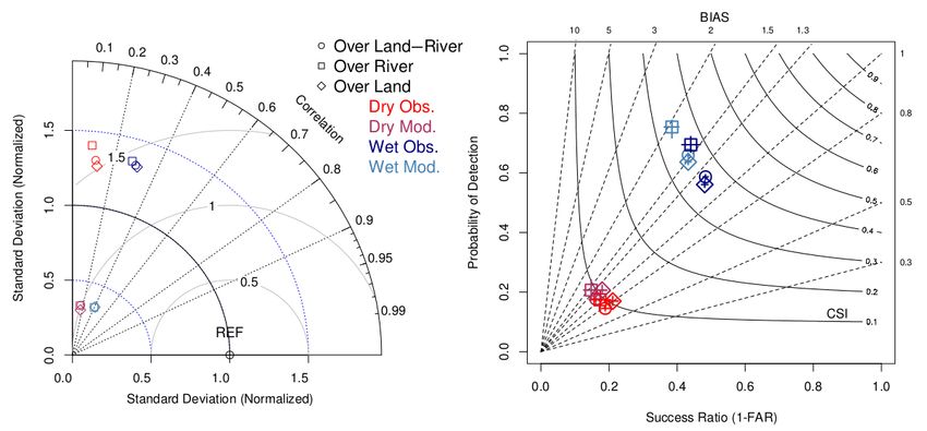
Remote Sens. Sens.10,
2018,
Remote 33610, x FOR PEER REVIEW
2018, 6 of 13 6 of 12
validation period, the reference PDF shape and magnitude are well reproduced (Figure 3). The
show low positive
differences (negative)
between values
estimated for the first
and observed PDFs,(second)
which areclass of observed
normalized precipitation
by the reference (between 0
probability
Remote Sens. 2018, 10, x FOR PEER REVIEW 6 of 13
mm·h−show
and 0.2density, 1 ). low positive (negative) values for the first (second) class of observed precipitation
(between 0 and
validation 0.2 mm∙h
period,
−1).
the reference PDF shape and magnitude are well reproduced (Figure 3). The
differences between estimated and observed PDFs, which are normalized by the reference probability
density, show low positive (negative) values for the first (second) class of observed precipitation
(between 0 and 0.2 mm∙h−1).
(a) (b) (c)
Figure 3. Histogram of the correct no-precipitation detection error (Case 0) for the 0.2 mm
Histogram of the correct no-precipitation detection error (Case 0) for the 0.2 mm h−1hthreshold
−1
Figure 3.
threshold over land–river (a), river only (b), and land only (c) during the dry (red) and wet (blue)
over land–river (a), river only (b), and land only (c) during the dry (red) and wet (blue) seasons. Bars
(a)
seasons. Bars indicate (b)
the observed probability density (c)represent the
function (PDF), dotted lines
indicatesimulated
the observed
PDF, andprobability
dashed linesdensity function
are the PDF (PDF),
differences dotted lines represent the simulated PDF,
(simulated–observed).
Figure 3. Histogram of the correct no-precipitation detection error (Case 0) for the 0.2 mm h−1
and dashed lines are the PDF differences (simulated–observed).
threshold over land–river (a), river only (b), and land only (c) during the dry (red) and wet (blue)
For Case 1, the frequency of several satellite rain rate classes (from 1 to 15 mm∙h−1) was compared
seasons. Bars indicate the observed probability density function (PDF), dotted lines represent the
to the observed precipitation distribution during the validation period (Figure 4). The dry–wet
For Casesimulated
1, the frequency of several
PDF, and dashed lines aresatellite classes (from 1 to 15 mm·h−1 ) was compared
rain rate (simulated–observed).
the PDF differences
performance difference is evident, especially for light precipitation. In the dry season, negative
to the observed
differences precipitation
(between 0.4 anddistribution
0.6) during the validation period (Figure 4).4 mm∙h
The −1dry–wet
For Case 1, the frequency of are observed
several forrain
satellite satellite precipitation
rate classes (from 1ranging from
to 15 mm∙h −1)1was
to compared
performance
and difference is evident, especially for land
light precipitation. AnIn the dry season, withnegative
to positive differences
the observed (~0.5) characterize
precipitation distributiontheduring
over theonly surface type.
validation period opposite
(Figure 4).behavior
The dry–wet
differences (between
a performance
large 0.4
overestimation and of 0.6)
the are
error observed
distributionsfor satellite
is observed precipitation
during the wetranging
period
difference is evident, especially for light precipitation. In the dry season, negative from
for all 1 to 4 mm·h−1
satellite
precipitation
and positive
differences classes. Moreover,
differences
(between (~0.5)
0.4 and Figure
are 4observed
characterize
0.6) showsthepoor
over performanceonlyatsurface
light rain
land precipitation
for satellite ratesfrom
type.
ranging (reference
to 4rainfall
An 1opposite mm∙h behavior
−1
~0.5 mm∙h −1) over river only, with underestimated (overestimated) probability densities by about 0.6
and positive differencesof(~0.5) characterize the over land only surface type. An
with a large overestimation the error distributions is observed during theopposite
wet periodbehavior
for with
all satellite
for almostoverestimation
a large all the satellite of
classes during
the error the dry (wet)
distributions is season.
observed during the wet period for all satellite
precipitation classes. Moreover, Figure 4 shows poor performance at light rain rates (reference rainfall
precipitation classes. Moreover, Figure 4 shows poor performance at light rain rates (reference rainfall
~0.5 mm·h−1 ) over river only, with underestimated (overestimated) probability densities by about 0.6
~0.5 mm∙h−1) over river only, with underestimated (overestimated) probability densities by about 0.6
for almost all the satellite classes during the dry (wet) season.
for almost all the satellite classes during the dry (wet) season.
(a) (b)
(a) (b)
(c) (d)
(c) (d)
(e) (f)
(e) (f)
Figure 4. Frequency differences (estimated–observed) (Case 1) for the dry (left) and wet (right)
validation periods and over land–river (a,b), river only (c,d), and land only (e,f), for threshold values
of satellite rain rates between 1.0 and 15.0 mm·h−1 .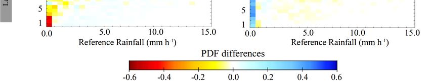
Remote Sens. 2018, 10, x FOR PEER REVIEW 7 of 13
Remote Sens.Figure 4. 336
2018, 10, Frequency differences (estimated–observed) (Case 1) for the dry (left) and wet (right) 7 of 12
validation periods and over land–river (a,b), river only (c,d), and land only (e,f), for threshold values
of satellite rain rates between 1.0 and 15.0 mm∙h−1.
The error spatial distributions were then investigated in order to better understand the
The error spatial distributions were then investigated in order to better understand the model
model performance over different surface types during one precipitation event in the dry season
performance over different surface types during one precipitation event in the dry season (06:30–06:59
(06:30–06:59 UTC on 28 May 2015) and one during the wet season (04:00–04:29 UTC on 12 March 2014).
UTC on 28 May 2015) and one during the wet season (04:00–04:29 UTC on 12 March 2014). Figures 5
Figures 5 and
and 6 show6 show (i) the observed
(i) the observed error (lefterror (left
panels), panels),as
computed computed as the
the difference difference
between IMERG between IMERG
and S-band
and S-band
SIPAM radar; the estimated error (middle panels), computed as the difference between the S-band the
SIPAM radar; the estimated error (middle panels), computed as the difference between
S-band SIPAM
SIPAM radar
radar and and the mean
the mean of theofmodeled
the modeled distribution;
distribution; andscatterplots
and (ii) the (ii) the scatterplots
of estimated ofversus
estimated
versus observed
observed errors
errors (right
(right panels),
panels), togethertogether
with thewith the corresponding
corresponding correlationcorrelation
coefficients. coefficients.
(a) (b) (c)
(d) (e) (f)
(g) (h) (i)
FigureFigure 5. Comparisons
5. Comparisons of observed
of observed andestimated
and estimated errors
errors during
duringa asingle
singletime
timestep (06:30–06:59
step UTCUTC
(06:30–06:59
on 28on 28 May
May 2015)2015)
overover land–river
land–river (a–c),river
(a–c), riveronly
only (d–f),
(d–f), and
andland
landonly
only(g–i), during
(g–i), duringthe the
dry dry
validation
validation
period. The observed error is defined as the difference between the Integrated Multisatellite
period. The observed error is defined as the difference between the Integrated Multisatellite Retrievals
Retrievals for Global Precipitation Measurement (IMERG) satellite retrieval and the S-band SIPAM
for Global Precipitation
radar observation. Measurement
The estimated error (IMERG) satellite
is defined retrievalbetween
as difference and the theS-band
satelliteSIPAM
and theradar
observation.
estimatedThe estimated
reference error is(not
precipitation defined as The
shown). difference between
scatterplots (c,f,i) the
showsatellite
estimatedand theversus
error estimated
observed
reference error.
precipitation (not shown). The scatterplots (c,f,i) show estimated error versus observed error.
PUSH adequately reproduced the spatial intensity patterns of the error in both precipitation
PUSH adequately reproduced the spatial intensity patterns of the error in both precipitation events.
events. Nevertheless, the error model clearly underestimates (~−0.5 mm∙h−1) light precipitation for
Nevertheless,
both the the
dryerror
and model clearlyThe
wet seasons. underestimates
estimated error(~−did
0.5 mm h−1 ) light precipitation
not ·reproduce for both the
correctly the satellite
dry and wet seasons. The estimated error did not reproduce correctly the satellite underestimations,
underestimations, presenting less underestimation than the observed error. On the other hand, the
presenting
model less
showsunderestimation
good performance than at
thelarge
observed error. when
rain rates, On the theother hand,
satellite the model
greatly shows good
overestimates
performance at large
precipitation. Therain rates, when
scatterplots the the
confirm satellite greatly
agreement overestimates
between observedprecipitation.
and estimated The scatterplots
errors, with
some
confirm theoverestimation of the error
agreement between at low
observed andsatellite rain rates.
estimated errors,The
withcorrelation coefficient presented
some overestimation of the error
at lowvalues between
satellite 0.93 and
rain rates. The0.96, slightly varying
correlation depending
coefficient on thevalues
presented surfacebetween
type conditions and0.96,
0.93 and season.
slightly
However, no remarkable difference in the model performance was observed for different conditions,
varying depending on the surface type conditions and season. However, no remarkable difference in
which shows independent calibration of the error model for different surface types and seasons.
the model performance was observed for different conditions, which shows independent calibration
of the error model for different surface types and seasons.
To further evaluate the PUSH performance, Figure 7 demonstrates its long-term ability to
reproduce the error in terms of intensity and spatial distribution. The standard deviation (SD) of
both the observed and estimated errors and their correlation coefficient (COR) were computed for the
validation dry and wet periods. In order to investigate the influence of the surface type on the error
spatial distribution, the over land and over river observed and estimated errors were combined and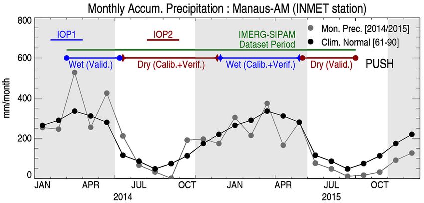
Remote Sens. 2018, 10, x FOR PEER REVIEW                                                                     8 of 13

           To further evaluate the PUSH performance, Figure 7 demonstrates its long-term ability to
Remote reproduce    the336
       Sens. 2018, 10,   error in terms of intensity and spatial distribution. The standard deviation (SD) of8 of 12
      both the observed and estimated errors and their correlation coefficient (COR) were computed for
      the validation dry and wet periods. In order to investigate the influence of the surface type on the
      error spatial
analyzed.           distribution,
            It is evident         the over
                            for both        landthat
                                      periods    and over  river observed
                                                     the modeled     errorand   estimated
                                                                             produced     errorsSD
                                                                                        lower    were combined
                                                                                                    values  than did
      and analyzed.
the observed          It is evident
                differences,        for bothless
                               indicating     periods
                                                 errorthat  the modeled
                                                       variability.       error produced
                                                                     However,             lower
                                                                                  the spatial    SD values than
                                                                                              distribution  patterns
      did the   observed   differences,  indicating less error  variability. However,   the spatial distribution
of the errors look similar to each other, regardless of the period. The wet period is also characterized
      patterns of the errors look similar to each other, regardless of the period. The wet period is also
by a higher   SD than is the dry one, when IMERG largely overestimates the precipitation observed
      characterized by a higher SD than is the dry one, when IMERG largely overestimates the
by the S-band SIPAM radar, especially along the river. The maximum SD values for the observed
      precipitation observed by the S-band −     SIPAM radar, especially along the river. The maximum SD
and modeled      errors are about 2.2 mm·h 1 and 2.0 mm·h−1 for the dry season and 3.0 mm·h−1 and
      values for the observed and modeled errors are about 2.2 mm∙h−1 and 2.0 mm∙h−1 for the dry season
2.5 mm  ·h−3.0
      and
            1 for the wet season, respectively. The spatial distributions of the temporal COR show most
                mm∙h−1 and 2.5 mm∙h−1 for the wet season, respectively. The spatial distributions of the
valuestemporal
        between    0.8show
                 COR   and 1most
                               during   both
                                   values      dry and
                                           between      wet 1periods.
                                                    0.8 and             However,
                                                               during both   dry andthe
                                                                                     wethighest
                                                                                          periods.COR   values
                                                                                                   However,  thewere
concentrated    along
      highest COR      the river
                     values  were and   during the
                                  concentrated      wet
                                                 along theseason.
                                                            river and during the wet season.

                                           (a)                    (b)                              (c)

                                           (d)                    (e)                              (f)

                                           (g)                    (h)                              (i)

              Figure 6. As in Figure 5, but for the wet validation period (04:00–04:29 UTC on 12 March 2014).
        Figure
     Remote Sens. 6. As10,
                  2018, inxFigure 5, but
                           FOR PEER      for the
                                     REVIEW        wet validation period (04:00–04:29 UTC on 12 March 2014).
                                                                                                         9 of 13

                                                 (a)                    (b)                  (c)

                                                 (d)                    (e)                  (f)

          Figure 7. Spatial distributions of the standard deviation of (a,d) observed and (b,e) estimated errors
     Figure 7. Spatial distributions of the standard deviation of (a,d) observed and (b,e) estimated errors
          and their (c,f) correlation coefficients over the dry (upper) and wet (lower) seasons.
     and their (c,f) correlation coefficients over the dry (upper) and wet (lower) seasons.
     3.3. Satellite Precipitation Product Correction
          The original IMERG product was then corrected using the PUSH modeled errors, according to
     the following relationship:
                                                         Xc = X + E                                                 (1)
     where Xc is the “corrected” IMERG rainfall estimates, X is the original IMERG rainfall estimates, and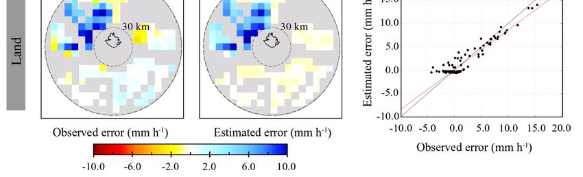
Remote Sens. 2018, 10, 336 9 of 12
3.3. Satellite Precipitation Product Correction
The original IMERG product was then corrected using the PUSH modeled errors, according to
the following relationship:
Xc = X + E (1)
where Xc is the “corrected” IMERG rainfall estimates, X is the original IMERG rainfall estimates, and E
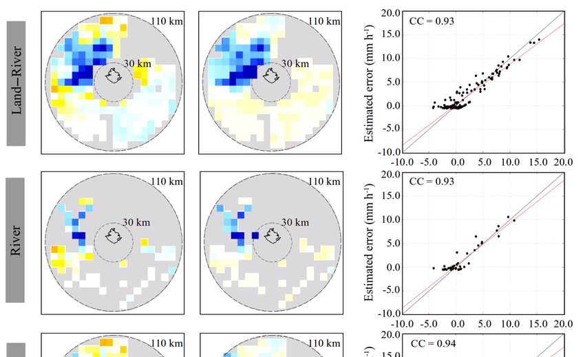
is the estimated error obtained via PUSH. The performance of the corrected IMERG was evaluated
for different surface types and seasons and compared with the original IMERG. Both continuous and
categorical scores were used as performance metrics and are shown in Figure 8 in the form of (i) a
Taylor diagram [27], which summarizes how closely a dataset matches a reference using COR, root
mean square error (RMSE), and SD; and (ii) a Performance diagram [28], which utilizes the geometric
relationship between success ratio (SR), which is represented by 1 − False Alarm Ratio (FAR), the
probability of detection (POD), bias score (BIAS), and the critical success index (CSI) to display all four
metrics simultaneously. A seasonal dependence, which is strongly linked to the precipitation regime
in the region, is observed in both the Taylor and Performance diagrams and corroborates the results in
Oliveira et al. [10]. The dry period presents a clear underperformance in comparison with the wetter
period, especially in the categorical metrics (Figure 8b).
The corrected IMERG presents a slightly better performance than does the original IMERG,
particularly in the continuous scores shown in the Taylor diagram. The COR for all the conditions
increased from ~0.1 to 0.2 during the dry period and from ~0.3 to 0.4 during the wet period. The most
notable improvement is observed in the normalized SD and RMSE scores. This indicates that the
corrected IMERG estimates are closer to the S-band radar rainfall estimates (reference) than are those
of the Sens.
Remote original
2018, IMERG
10, x FOR product.
PEER REVIEW 10 of 13
(a) (b)
Figure 8.
Figure 8. Taylor
Taylordiagram
diagram (a)(a) and
and performance
performance diagram
diagram (b) showing
(b) showing dry anddrywet
and wet metrics
metrics of the
of the IMERG
IMERG original rainfall estimates versus IMERG modeled via the PUSH model, for
original rainfall estimates versus IMERG modeled via the PUSH model, for different surface types overdifferent surface
types
the over the
Manaus Manaus
region region
and for and for the
the validation validation
period. In (a),period. In (a),
the angular theshow
axes angular
COR; axes show radial
whereas COR;
whereas
axes (blueradial
lines)axes
show (blue lines)
the SD, show the against
normalized SD, normalized against
the reference; andthethereference; and the
centered RMS centered
difference is
RMS difference
represented is represented
by the by In
solid gray line. the(b),
solid graylines
dashed line. represent
In (b), dashed lines with
bias scores represent
labelsbias scores
on the with
outward
labels on the
extension outward
of the extension
line; the of thecontours
labeled solid line; the correspond
labeled solid tocontours correspond
CSI; the x- and y-axistorepresent
CSI; the the
x- and
SR
y-axis represent the SR and POD, respectively; and sampling
and POD, respectively; and sampling uncertainty is given by the crosshairs.uncertainty is given by the crosshairs.
4. Discussion
4. Discussion
The novelty of
The novelty this study
of this study consists
consists in
in investigating
investigating the error characteristics
the error characteristics of
of the recently
the recently
developed IMERG
developed IMERGrainfall
rainfallproducts
products over
over a tropical
a tropical area area characterized
characterized by distinct
by distinct surfacesurface type
type classes
classes (e.g., forest, nonforest, hydrology, and urban areas), i.e., the central Amazon region.
Specifically, this work proposes a novel framework to correct these estimates that have the potential
to be used in hydrological predictions and water resource management across the globe. In order to
expand our results to other regions, a seasonal surface-type-based analysis was performed.
During the calibration period, PUSH presented promising results for estimating the error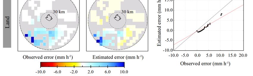
Remote Sens. 2018, 10, 336                                                                           10 of 12

(e.g., forest, nonforest, hydrology, and urban areas), i.e., the central Amazon region. Specifically, this
work proposes a novel framework to correct these estimates that have the potential to be used in
hydrological predictions and water resource management across the globe. In order to expand our
results to other regions, a seasonal surface-type-based analysis was performed.
      During the calibration period, PUSH presented promising results for estimating the error
associated with satellite rainfall products at moderate to heavy rainfall rates, as shown by results in
Section 3.1. The validation results presented in Section 3.2 suggest that the PUSH error model could
efficiently characterize the IMERG error along the Negro, Solimões, and Amazon rivers, especially
during the wet season. Furthermore, results presented in Section 3.3 showed that the PUSH-corrected
IMERG exhibited improvements in the continuous statistics with respect to the original IMERG dataset.
However, no significant improvements were observed in the categorical statistics, which suggests
that the ability to detect local characteristics, especially during the dry season (i.e., local convection)
depends more on the physical assumptions within the satellite rainfall retrieval algorithms. One
option would be, for instance, to exploit other passive microwave channels to minimize the uncertainty
related to the bright band for surface rainfall retrievals, among others.
      Such findings are of fundamental importance to the correct and successful application of
GPM-based rainfall estimates in several applications, like natural disaster monitoring, data assimilation
systems, hydrological modeling, climatic studies, and for better understanding of the physical
processes of precipitation systems over the Amazon region. Moreover, our results provide useful
information for satellite precipitation algorithm developers and contribute to meliorating the
GPM products.

5. Conclusions
       In this study, the characteristics of errors associated with the GPM IMERG final product were
investigated over the central Amazon region using an S-band radar as reference. The analysis was
performed comparing the dry and wet seasons during March 2014 and August 2015. The PUSH error
framework, originally proposed by Maggioni et al. [8], was calibrated and validated for the study
region, and expanded to take into account local factors like seasonality and surface types (i.e., land
and river).
       Results showed that the PUSH model was able to reproduce the error between the IMERG product
and the S-band SIPAM radar ground observations. During the calibration period, PUSH could capture
the overall spatial pattern of precipitation for both seasons and surface types. However, the model
exhibited limited capability in characterizing light precipitation and associated errors. For Case 0
(i.e., when the satellite product detects no rain), PUSH slightly overestimated the rainfall during both
dry and wet seasons. A slight (but not significant) overestimation of light rain rates was also observed
for Case 1 (i.e., when the satellite product detects rain) for all conditions. During the validation period,
PUSH was able to efficiently predict the error distributions during dry and wet periods. However, an
underestimation (overestimation) of light rain rates was observed during the dry (wet) period. Such
behavior was clearly detected in Case 0 (for rain rate classes lower than 0.2 mm·h−1 ) and for Case 1,
especially over the river.
       Overall, the PUSH-modeled error presented similar spatial and intensity distributions when
compared with the observed error. Although the estimated errors have a lower standard deviation
than the observed error, there is a high correlation between the two and a good capability in capturing
the error along the Negro, Solimões, and Amazon rivers, especially during the wet season. Lastly, the
PUSH-corrected IMERG product presented a slight improvement with respect to the original IMERG
dataset during the validation period. The improvement was more evident in the continuous statistical
metrics than in the categorical ones. Future studies should focus on investigating and separating the
random and systematic error components and on verifying the viability of using PUSH to correct
IMERG products in other regions of Brazil and beyond.
Remote Sens. 2018, 10, 336 11 of 12
Supplementary Materials: The following are available online at www.mdpi.com/2072-4292/10/2/336/s1.
Figure S1. Probability of false alarm (P10) (upper panels) and probability of hit (P11) (lower panels) for a minimum
threshold of 0.2 mm·h−1 over land–river (green), over river only (red), and over land only (blue), during the dry
(left panels) and wet (right panels) seasons. Figure S2. Distributions of correct no-precipitation detection errors
(Case 0) for the 0.2 mm·h−1 threshold over land–river (a), over river only (b), and over land only (c), during the
dry (red) and wet (blue) seasons (calibration period). Bars indicate the observed PDF, dotted lines represent the
simulated PDF, and dashed lines show the PDF differences (simulated–observed). Figure S3. PDF from observations
(bars) and simulated by the error model (black lines) and their differences (estimated minus observed probability
densities) for the dry (in red) and wet (in blue) calibration periods and over land–river (a,d), over river only (b,e),
and over land only (c,f). Examples for threshold values of satellite rain rates of 2.5 and 10.0 mm·h−1 .
Acknowledgments: The first author acknowledges financial support from the National Council for Scientific and
Technological Development (CNPq) and the Coordination for the Improvement of Higher Education Personnel
(CAPES) Brazil during his PhD. studies and also the Institutional Program of Overseas Sandwich Doctorate (PDSE)
from CAPES (process 6836-15-1) for the internship opportunity. The authors also acknowledge the CHUVA Project
(FAPESP Grant 2009/15235-8), the Amazon Protection National System (SIPAM), Texas A&M University (TAMU),
and NASA/Goddard Space Flight Centers and Precipitation Processing System (PPS) for the data provided for
this study, and Aaron Funk and Mári Firpo for the data and methodology support. The IMERG datasets are
provided by NASA/PPS and are available at https://pmm.nasa.gov/data-access/downloads/gpm. The ground
radar data from SIPAM/TAMU are available at http://chuvaproject.cptec.inpe.br.
Author Contributions: Rômulo Oliveira designed the study, conducted the analysis and wrote the manuscript.
Viviana Maggioni, Daniel Vila, and Leonardo Porcacchia contributed to discussions and revisions, providing
important feedback and suggestions.
Conflicts of Interest: The authors declare no conflict of interest.
References
1. Espinoza, C.; Marengo, J.A.; Ronchail, J.; Carpio, J.M.; Flores, L.N.; Guyot, J.L. The extreme 2014 flood in
south-western Amazon basin, the role of tropical-subtropical South Atlantic SST gradient. Environ. Res. Lett.
2014, 9, 124007. [CrossRef]
2. Falck, A.S.; Maggioni, V.; Tomasella, J.; Vila, D.A.; Diniz, F.L.R. Propagation of satellite precipitation
uncertainties through a distributed hydrologic model: A case study in the Tocantins-Araguaia basin in Brazil.
J. Hydrol. 2014, 527, 943–957. [CrossRef]
3. de Oliveira, N.S.; Rotunno Filho, O.C.; Marton, E.; Silva, C. Correlation between rainfall and landslides in
Nova Friburgo, Rio de Janeiro-Brazil: A case study. Environ. Earth Sci. 2016, 75, 1358. [CrossRef]
4. Hong, Y.; Hsu, K.-L.; Moradkhani, H.; Sorooshian, S. Uncertainty quantification of satellite precipitation
estimation and monte carlo assessment of the error propagation into hydrologic response. Water Resour. Res.
2006, 42, 1–15. [CrossRef]
5. Tang, L.; Tian, Y.; Yan, F.; Habib, E. An improved procedure for the validation of satellite-based precipitation
estimates. Atmos. Res. 2015, 163, 61–73. [CrossRef]
6. Tian, Y.; Huffman, G.J.; Adler, R.F.; Tang, L.; Sapiano, M.; Maggioni, V.; Wu, H. Modeling errors in daily
precipitation measurements: Additive or multiplicative? Geophys. Res. Lett. 2013, 40, 2060–2065. [CrossRef]
7. Tian, Y.; Peters-Lidard, C.; Eylander, J.; Joyce, R.; Huffman, G.; Adler, R.; Hsu, K.; Turk, F.; Garcia, M.
Component analysis of errors in satellite-based precipitation estimates. J. Geophys. Res. 2009, 114, D24101.
[CrossRef]
8. Maggioni, V.; Sapiano, M.; Adler, R.; Tian, Y.; Huffman, G. An error model for uncertainty quantification in
high-time-resolution precipitation products. J. Hydrometeorol. 2014, 15, 1274–1292. [CrossRef]
9. Maggioni, V.; Sapiano, M.R.P.; Adler, R.F. Estimating uncertainties in high-resolution satellite precipitation
products: Systematic or random error? J. Hydrometeorol. 2016, 17, 1119–1129. [CrossRef]
10. Oliveira, R.; Maggioni, V.; Vila, D.; Morales, C. Characteristics and diurnal cycle of GPM rainfall estimates
over the central Amazon region. Remote Sens. 2016, 8, 544. [CrossRef]
11. Burleyson, C.; Feng, Z.; Hagos, S.; Fast, J.; Machado, L.; Martin, S. Spatial Variability of the Background
Diurnal Cycle of Deep Convection around the GoAmazon2014/5 Field Campaign Sites. J. Appl. Meteorol.
Climatol. 2016. [CrossRef]
12. Giangrande, S.E.; Toto, T.; Jensen, M.P.; Bartholomew, M.J.; Feng, Z.; Protat, A.; Williams, C.R.;
Schumacher, C.; Machado, L. Convective cloud vertical velocity and mass-flux characteristics from radar
wind profiler observations during GoAmazon2014/5. J. Geophys. Res. Atmos. 2016, 121, 891–913. [CrossRef]Remote Sens. 2018, 10, 336 12 of 12
13. Tang, S.; Xie, S.; Zhang, Y.; Zhang, M.; Schumacher, C.; Upton, H.; Jensen, M.P.; Johnson, K.L.; Wang, M.;
Ahlgrimm, M.; et al. Large-scale vertical velocity, diabatic heating and drying profiles associated with
seasonal and diurnal variations of convective systems observed in the GoAmazon2014/5 experiment.
Atmos. Chem. Phys. 2016, 16, 14249–14264. [CrossRef]
14. Huffman, G.J.; Bolvin, D.T.; Braithwaite, D.; Hsu, K.; Joyce, R.; Xie, P. GPM Integrated Multi-Satellite
Retrievals for GPM (IMERG) Algorithm Theoretical Basis Document (ATBD); National Aeronautics and Space
Administration (NASA): Washington, DC, USA, 2015. Available online: http://pmm.nasa.gov/sites/
default/files/document_files/IMERG_ATBD_V4.4.pdf (accessed on 10 August 2016).
15. Huffman, G.J.; Bolvin, D.T.; Nelkin, E.J. Integrated Multi-Satellite Retrievals for GPM (IMERG) Technical
Documentation; National Aeronautics and Space Administration (NASA): Washington, DC, USA, 2015.
Available online: http://pmm.nasa.gov/sites/default/files/document_files/IMERG_doc.pdf (accessed on
10 August 2016).
16. Machado, L.A.T.; Silva Dias, M.A.F.; Morales, C.; Fisch, G.; Vila, D.; Albrecht, R.; Goodman, S.J.;
Calheiros, A.J.P.; Biscaro, T.; Kummerow, C.; et al. The CHUVA Project. How Does Convection Vary
across Brazil? Bull. Am. Meteorol. Soc. 2014, 95, 1365–1380. [CrossRef]
17. Martin, S.T.; Artaxo, P.; Machado, L.A.T.; Manzi, A.O.; Souza, R.A.F.; Schumacher, C.; Wang, J.; Andreae, M.O.;
Barbosa, H.M.J.; Fan, J.; et al. Introduction: Observations and Modeling of the Green Ocean Amazon
(GoAmazon2014/5). Atmos. Chem. Phys. 2016, 16, 4785–4797. [CrossRef]
18. Marengo, J.A.; Fisch, G.F.; Alves, L.M.; Sousa, N.V.; Fu, R.; Zhuang, Y. Meteorological context of the onset
and end of the rainy season in Central Amazonia during the GoAmazon2014/5. Atmos. Chem. Phys. 2017, 17,
7671–7681. [CrossRef]
19. Liebmann, B.; Marengo, J. Interannual variability of the rainy season and rainfall in the Brazilian Amazon
Basin. J. Clim. 2001, 14, 4308–4318. [CrossRef]
20. Machado, L.; Laurent, H.; Dessay, N.; Miranda, I. Seasonal and diurnal variability of convection over the
Amazonia: A comparison of different vegetation types and large scale forcing. Theor. Appl. Climatol. 2004, 78,
61–77. [CrossRef]
21. Satyamurty, P.; De Castro, A.A.; Tota, J.; Gularte, L.E.S.; Manzi, A.O. Rainfall trends in the Brazilian Amazon
basin in the past eight decades. Theor. Appl. Climatol. 2010, 99, 139–148. [CrossRef]
22. Santos, E.B.; Lucio, P.S.; Silva, C.M.S. Precipitation regionalization of the Brazilian Amazon. Atmos. Sci. Lett.
2015, 16, 185–192. [CrossRef]
23. Villar, J.C.E.; Ronchail, J.; Guyot, J.L.; Cochonneau, G.; Naziano, F.; Lavado, W.; Oliveira, E.D.; Pombosa, R.;
Vauchel, P. Spatio-temporal rainfall variability in the Amazon basin countries (Brazil, Peru, Bolivia, Colombia,
and Ecuador). Int. J. Climatol. 2009, 29, 1574–1594. [CrossRef]
24. Liebmann, B.; Camargo, S.J.; Seth, A.; Marengo, J.A.; Carvalho, L.M.; Allured, D.; Fu, R.; Vera, C.S. Onset
and End of the Rainy Season in South America in Observations and the ECHAM 4.5 Atmospheric General
Circulation Model. J. Clim. 2007, 20, 2037–2050. [CrossRef]
25. Bombardi, R.J.; Carvalho, L.M.V. IPCC global coupled model simulations of the South America monsoon
system. Clim. Dyn. 2009, 33, 893–916. [CrossRef]
26. Coelho, C.A.S.; Cardoso, D.H.F.; Firpo, M.A.F. Precipitation diagnostics of an exceptionally dry event in
Sao Paulo, Brazil. Theor. Appl. Climatol. 2016, 125, 769–784. [CrossRef]
27. Taylor, K.E. Summarizing multiple aspects of model performance in a single diagram. J. Geophys. Res. 2001,
106, 7183–7192. [CrossRef]
28. Roebber, P.J. Visualizing multiple measures of forecast quality. Weather Forecast. 2009, 24, 601–608. [CrossRef]
© 2018 by the authors. Licensee MDPI, Basel, Switzerland. This article is an open access
article distributed under the terms and conditions of the Creative Commons Attribution
(CC BY) license (http://creativecommons.org/licenses/by/4.0/).You can also read