Jet-like features of Jiulongjiang River plume discharging into the west Taiwan Strait
←
→
Page content transcription
If your browser does not render page correctly, please read the page content below
Front. Earth Sci. 2013, 7(3): 282–294
DOI 10.1007/s11707-013-0372-0

  RESEARCH ARTICLE

    Jet-like features of Jiulongjiang River plume discharging
                    into the west Taiwan Strait

                                  Daifeng WANG1, Quan’an ZHENG1,2, Jianyu HU (✉)1
  1 State Key Laboratory of Marine Environmental Science, College of Ocean and Earth Sciences, Xiamen University, Xiamen 361005, China
                 2 Department of Atmospheric and Oceanic Science, University of Maryland, College Park, MD 20742, USA

© Higher Education Press and Springer-Verlag Berlin Heidelberg 2013

Abstract In-situ data from the summer cruise of 2010 in              1     Introduction
the west Taiwan Strait are used to study the spatial
distribution of the Jiulongjiang River plume (JRP). The              The Jiulongjiang River is the second largest river in Fujian
results show that in the 2 m layer, the JRP debouches into           Province in southeastern China, located on the west coast
the west Taiwan Strait in the form of jets, with one branch          of the Taiwan Strait. It consists of three tributaries: the
through the Xiamen Bay (Xiamen JRP) and another                      North Brook, the West Brook, and the South Brook
through the channel between Jinmen and Weitou (JinWei                (Fig. 1). The North Brook is the main stream with annual
JRP). Driven by the summer southwesterly monsoon, the                mean runoff reaching 8:9  109 m3, and the West Brook
upwelling-related Dongshan low temperature and high
                                                                     has an annual mean runoff of 3:7  109 m3. The combined
salinity water flows northeastward in the form of a jet as
                                                                     peak discharge of the two brooks in the wet season from
well. To a certain degree, the Dongshan low temperature
                                                                     April to September accounts for 74% of the total annual
and high salinity jet restricts the Xiamen JRP from
                                                                     runoff. The Jiulongjiang River runoff is mainly affected by
spreading further offshore and drags the JinWei JRP
                                                                     precipitation, and heavy flooding may be caused by
northeastward at the same time. Meanwhile, a terrestrial
                                                                     rainstorms and typhoon rainfall (Guo et al., 2011).
dissolved organic matter (DOM) distribution model on the
                                                                        The river discharges to coastal waters with a large
basis of molecular collision theory in thermodynamics and
                                                                     amount of nutrients, sediments, and contaminants have
statistical physics is applied to analyze the Moderate
                                                                     profound influence on the sensitive coastal marine
Resolution Imaging Spectroradiometer (MODIS) turbidity
                                                                     ecosystems. Hydrodynamically, the fresh river water
data. The correlation coefficient of the theoretical model to
                                                                     spreading over the saline seawater forms a body of
the MODIS turbidity data reaches 0.96 (significant at a
                                                                     plumose low salinity water, which is generally called
95% level of confidence). The result clarifies the dynamic
                                                                     plume. The river plume constitutes an important dynamic
mechanism for the turbidity distribution characteristics. It
                                                                     component of the coastal circulation. Due to ecological and
is the salinity in macro-scale that plays a decisive role in
                                                                     dynamical importance, it is necessary to have a good
the turbidity variability in the coastal water. This suggests
                                                                     understanding of river plumes. However, to a great extent,
that the satellite-derived turbidity data can be used as an
                                                                     interest in river plumes has only focused on large rivers,
indicator to show the spreading patterns of the JRP. Based
                                                                     such as the Yangtze River (Mao et al., 1963; Lie et al.,
on the turbidity data from 2003 to 2011, we conclude that
                                                                     2003; Kim et al., 2009; Wu et al., 2011; Rong and Li,
there are four main spreading patterns of the JRP.
                                                                     2012), the Mississippi River (Ortner et al., 1995; Schiller et
                                                                     al., 2011), and the Columbia River plume (Hickey et al.,
Keywords Jiulongjiang River plume, jet current, terres-
                                                                     2005; Liu et al., 2009a, 2009b; MacCready et al., 2009).
trial DOM, MODIS data, Taiwan Strait
                                                                     For the small rivers such as the Jiulongjiang River, the
                                                                     previous investigators mainly paid attention to the area
                                                                     from the river mouth to the Xiamen Bay, focusing on the
                                                                     distribution characteristics of the salinity, the salinity front,
                                                                     the changes in nutrients and the impact of tides to the
                                                                     characteristics (Zhang et al., 1999; Chen et al., 2002; Luo
Received January 18, 2013; accepted March 6, 2013                    et al., 2011, 2012). The sediment transport, chlorophyll a
E-mail: hujy@xmu.edu.cn                                              and primary productivity, and current fields were also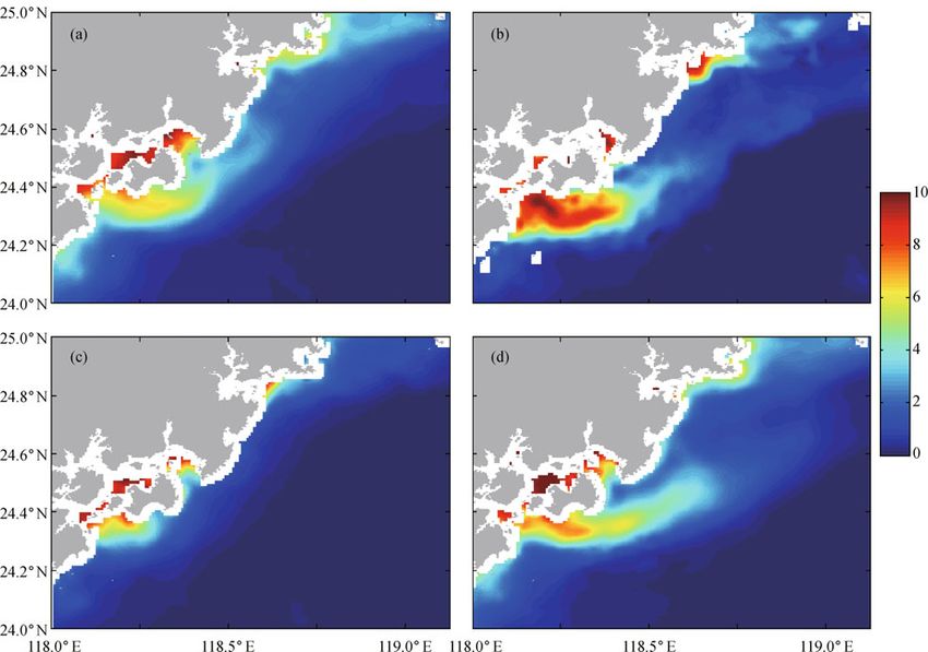
Daifeng WANG et al. Jet-like Jiulongjiang River plume discharging into the west Taiwan Strait                       283

      Fig. 1 Study area. Dots with codes represent CTD stations. Bathymetry units are in meter. XZ, SH, WT, JM, XM, NB, WB, ZHJ and DS
      represent Xiangzhi, Shenhu, Weitou, Jinmen, Xiamen, North Brook, West Brook, Zhenghaijiao, and Dongshan, respectively.

considered. In addition, the previous works on analyzing               density anomaly originally measured with a CTD profiler.
the data of temperature and salinity in the Taiwan Strait              As shown in Fig. 1, the survey area is mapped by the CTD
(Chen et al., 2002; Chen et al., 2009) involved the                    profiler casts at 49 sampling stations along 9 cross-shelf
hydrological characteristics of the Jiulongjiang River                 transects. The distance between two neighboring transects
plume (JRP). However, the dynamical characteristics of                 is about 18 km, and that between two adjacent stations
the JRP remain unclear. This study aims to clarify the                 varies from 8 to 15 km. At each station, the CTD data were
dynamical characteristics of the JRP using the cruise data             measured continuously from the sea surface to the depth
observed with a conductivity-temperature-depth (CTD)                   close to the bottom with a vertical resolution of 1 m.
profiler, the reanalyzed satellite turbidity data, and the              Because the lengths of transects are different, the sampling
theory of fluid mechanics, and that of molecular collision              time was from 4 to 5 h per transect, and the entire sampling
in thermodynamics and statistical physics.                             was accomplished in three days. The water depth in the
   We introduce the data used in this paper in Section 2,              survey area changes from 10 to 60 m (Fig. 1).
including the cruise data in summer 2010 and the Moderate                 In the meantime, based on the MODIS level 2 LAC
Resolution Imaging Spectroradiometer (MODIS) reana-                    (Large Area Collectors) data downloaded from the data
lyzed turbidity data. The analysis and interpretation of the           dissemination center of US NASA (National Aeronautics
in-situ salinity distribution are given in Section 3. Next, we         and Space Administration) Goddard Space Flight Center
investigate the distribution of terrestrial dissolved organic          (GSFC)1) and the algorithms used by Huang et al. (2008),
matter (DOM) of the JRP using the MODIS reanalyzed                     the turbidity data is calculated from 2003 to 2011 with a
turbidity data in Section 4. We do a statistical analysis of           spatial resolution of 1 km.
the turbidity data by using turbidity as an indicator of
plume in Section 5. Section 6 presents a summary.
                                                                       3     Cruise data analysis and interpretation
2    Data                                                              3.1    Spatial distribution of the JRP

The in-situ data used in this study are from the cruise                We use the cruise data to map the distributions of the
observations carried out from June 28 to 30 in 2010 in the             salinity and the temperature in 2 m layer and the salinity at
west Taiwan Strait, including the temperature, salinity, and           depths of 7 and 10 m. The results are shown in Figs. 2 and

1)   http://oceancolor.gsfc.nasa.gov/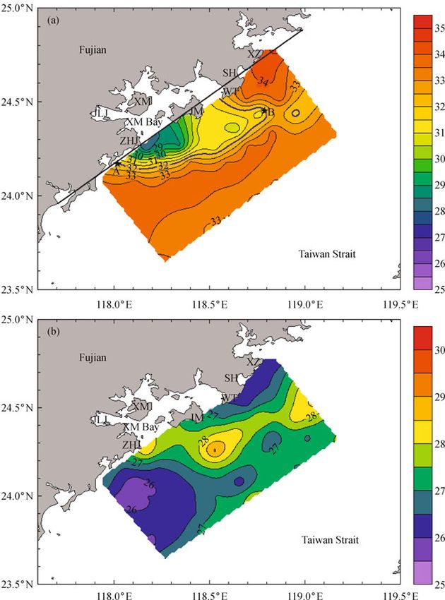
284                                                    Front. Earth Sci. 2013, 7(3): 282–294

      Fig. 2 Distributions of the salinity (a) and the temperature (b) at the depth of 2 m. Blue curve represents the 32 isohaline. Pentagrams
      represent the locations of points A (24.16°N, 118.00°E) and B (24.45°N, 118.79°E). Black bold line represents the general direction of
      coastline. In this figure, XZ, SH, WT, JM, XM, JLJ, and ZHJ represent Xiangzhi, Shenhu, Weitou, Jinmen, Xiamen, the Jiulongjiang
      River, and Zhenghaijiao, respectively.

3, respectively. Following the definition of the Yangtze                     reach the points of A and B (Fig. 2(a)), respectively, and
River plume (Mao et al., 1963), we define the 32 isohaline                   the two points are approximately 86.3 km apart.
contour as the boundary of the JRP.                                            In the survey area, driven by the summer southwesterly
   From Fig. 2, one can see that under the influence of                      monsoon, the sea water in the Dongshan upwelling zone
topography, the JRP debouches into the west Taiwan Strait                   (Chen et al., 1982; Hong et al., 2009a; Zhang et al., 2011)
through the Xiamen Bay and the channel between Jinmen                       flows northeastward, so that there is a low temperature and
and Weitou with high temperature and low salinity, varying                  high salinity tongue (Dongshan low temperature and high
from 25.7°C to 29.0°C and from 28.1 to 32.0, respectively.                  salinity water) running southwest-northeastward as shown
The maximum width between the JRP boundary (32                              in Fig. 2. The tongue axis is generally at an angle of 9° to
isohaline) and the coastline is about 31.5 km, with the                     the direction of coastline. After entering into the sea, the
direction of coastline defined as the black bold line shown                  JRP interacts with the tongue, making the isohalines
in Fig. 2(a). The most southwestern and northeastern edges                  become dense at the interaction zone. The horizontal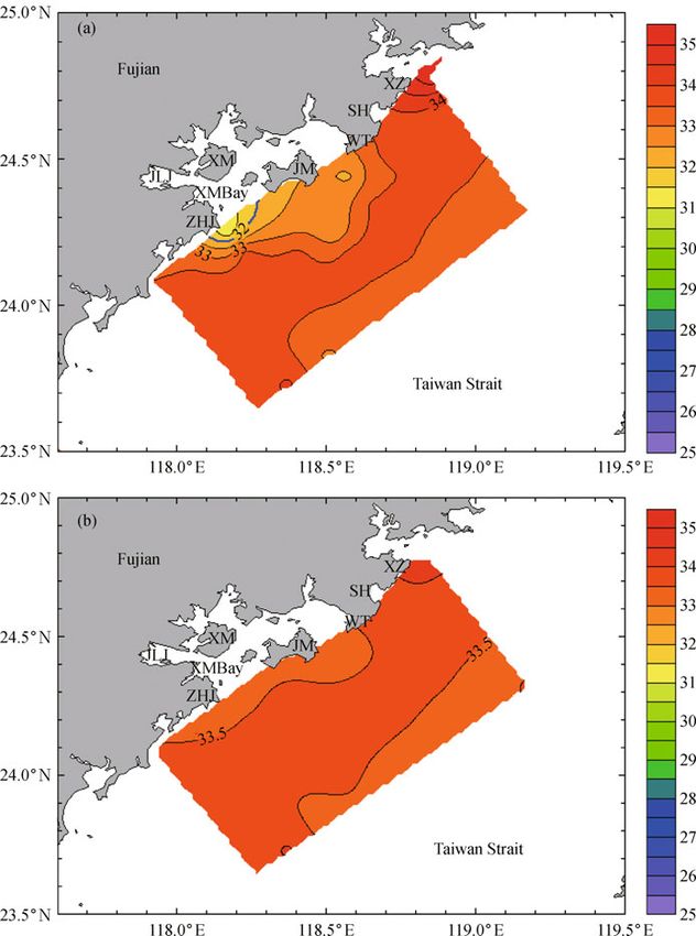
Daifeng WANG et al. Jet-like Jiulongjiang River plume discharging into the west Taiwan Strait                                285

    Fig. 3 Distributions of the salinity at 7 m (a) and 10 m (b). Blue bold line represents the 32 isohaline. In this figure, XZ, SH, WT, JM,
    XM, JLJ, and ZHJ represent Xiangzhi, Shenhu, Weitou, Jinmen, Xiamen, the Jiulongjiang River and Zhenghaijiao, respectively.

salinity gradient reaches 0.250/km, greatly exceeding the                 water with a salinity front is formed near the Xiamen Bay
criterion of 0.018/km for a salinity front (Hong et al.,                  mouth. There are two low salinity tongues in the plume:
2009b).                                                                   one is in the southwestward direction with an angle of 151°
   There is also a low temperature and high salinity tongue               to the direction of coastline, and the other is perpendicular
near the Xiangzhi-Weitou coastal area which is closely                    to the direction of coastline, pointing southeastward.
related to the local upwelling. The JRP interacts with the                   The low salinity tongue of the JRP entering into the west
tongue, making the horizontal salinity gradient reach                     Taiwan Strait through the channel between Jinmen and
0.180/km in the upwelling divergence region and forming                   Weitou (JinWei JRP) is sandwiched by high salinity waters
salinity fronts.                                                          on both shallow and deep water sides. The high salinity
   A river plume is usually characterized by a stable                     waters originate from the coastal upwelling near the
stratification with plume-induced fronts surfacing offshore                Xiangzhi-Weitou coastal area and the Dongshan low
(Chao and Boicourt, 1986). The maximum horizontal                         temperature and high salinity water, respectively. Isoha-
salinity gradient of the JRP discharging into the west                    lines on both sides of the JRP tongue are dense, with
Taiwan Strait through the Xiamen Bay (Xiamen JRP)                         maximum horizontal salinity gradients reaching 0.240/km
reaches 0.365/km. So we can conclude that the plume                       on the shallow water side and 0.180/km on the deep water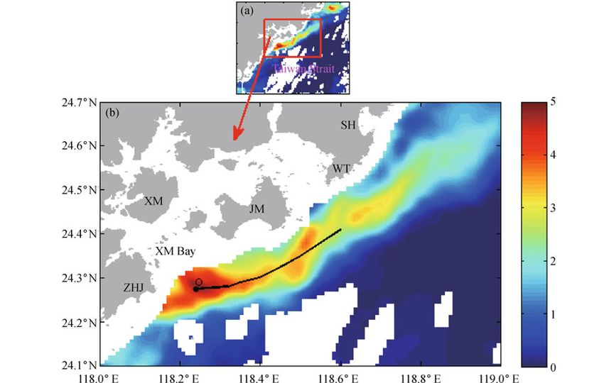
286                                                  Front. Earth Sci. 2013, 7(3): 282–294

side. This implies that the JinWei JRP forms a plume with a               From Eq. (2), we derive the velocity components of the
salinity front.                                                        jet. The x-component or axial velocity is given by
   Vertically, at the 7 m layer, the signal of the JRP also
exists as shown in Fig. 3(a), but the patterns differ from                                    u ¼ umax sech2 η,                     (6)
that at the 2 m layer. The 7 m layer of the JRP spreads near           where umax is the maximum axial velocity at the center of
the Xiamen Bay mouth, with the maximum width between                   the jet given by
its boundary (32 isohaline) and the coastline equaling
7.2 km and the width between the most southwestern and                                                     1=3
                                                                                         a            3M 2
the most northeastern edges approximating 17.5 km. The                            umax ¼ x – 1=3 ¼               x – 1=3 ,   (7)
                                                                                         b           322 v
tongue axis of the JRP in the 7 m layer coincides with that
of the JRP running southwestward in the 2 m layer, while               and the y-component or transverse velocity is given by
the tongue axis becomes a little shorter in the 7 m layer.
Thus, it is clear that the coverage of the JRP in this layer                            v ¼ vmax ð2ηsech2 η – tanh ηÞ,              (8)
becomes narrower. The maximum horizontal salinity                      where vmax is the maximum transversal velocity given by
gradient of the JRP in the 7 m layer reaches 0.243/km,
                                                                                                     a
which indicates that the plume water with a front is formed.                                   vmax ¼ x – 2=3 :                     (9)
Different from that in the 2 m layer, the direction of low                                           3
salinity tongue in the plume is single in the 7 m layer. At               From these equations, it follows that the dynamics of an
the 10 m layer, the plume signal disappears (Fig. 3(b)),               ideal two-dimensional jet are characterized by (i) a jet axis
implying that the JRP is mainly concentrated in the upper              that is kept unchanged, (ii) a jet width that increases as x2=3 ,
layers from the sea surface to the depth less than 10 m.
                                                                       (iii) an x-component velocity that decreases as x – 1=3 , and
3.2     Interpretation to the JRP distribution                         (iv) a y-component velocity that decreases as x – 2=3 (Zheng
                                                                       et al., 2004).
3.2.1    Two-dimensional jet

Formally, a two-dimensional jet is a special flow formed by
an efflux of fluid from a long and narrow orifice into the
same type of fluid as the jet itself, as illustrated in Fig. 4
(Kundu, 1990). Dynamically, the jet is controlled by two
conditions (Kundu, 1990). One is the momentum flux
preservation, i.e.,
                                 þ1

                         M ¼     ! u2dy,                       (1)
                                  –1

where ρ is the density of fluid, u is the x-component of                   Fig. 4 A scheme of a two-dimensional jet flow (redrawn from
velocity, and the coordinate system is defined as that in Fig.             Kundu, 1990).
4. The second condition is a similarity solution of the
stream function in the form of

                        ψ ¼ ax1=3 tanh η,                       (2)    3.2.2   Interpretation to the distribution of JRP

where                                                                  We use density anomaly (t ) data derived from the cruise
                                         1=3                         CTD measurements to calculate the current field structure.
                                9AH M                                  If we assume the y-component of velocity is ignored, the
                       a¼                        ,              (3)
                                  2                                   following approximate relation stands:
in which AH is the horizontal eddy viscosity, and                                              t ¼ – αuðyÞ,                       (10)
                                    y                                  where α is a constant to be determined and u(y) represents
                            η¼          ,                       (4)
                                  bx2=3                                the x-component of velocity. This means that using density
in which                                                               anomaly data we may determine a normalized form of u(y)
                                                                       used for dynamical analysis even though α is unknown
                                         1=3
                                48A2H                                 (Zheng et al., 2004). In this paper, we choose the JRP
                       b¼                        :              (5)    tongue axes and the upwelling-related low temperature and
                                  M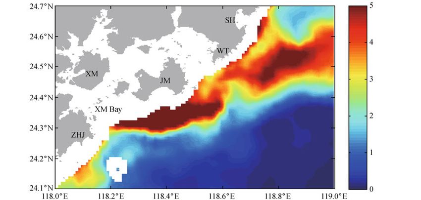
Daifeng WANG et al. Jet-like Jiulongjiang River plume discharging into the west Taiwan Strait                                   287

high salinity tongue axis as the x-axes, and the lines                      and a red arrow J1, respectively. Meanwhile, the JinWei
perpendicular to x-axes are y-axes.                                         JRP enters into the west Taiwan Strait also in the form of
   In order to compare the velocity fields of the JRP with                   jet J2 whose axis points northeastward shown as a black
those of the corresponding jet models, we select two                        arrow J2 in Fig. 5 with an angle of 9° to the direction of
transects off Zhenhaijiao-Jinmen and another two transects                  coastline.
off Jinmen-Shenhu, defined as T0 (blue line in Fig. 5), T1                      Similarly, in order to compare the velocity field of the
(red line in Fig. 5), T2-1 and T2-2 (black lines in Fig. 5),                Dongshan low temperature and high salinity water in the 2
respectively. T0 includes two stations X51 and X60 and                      m layer with that of the corresponding jet model, we select
one interpolation point (blue dot in Fig. 5) whose density                  two transects, T3-1 and T3-2, shown as purple lines in Fig.
anomaly data is calculated by using linear interpolation                    5. Stations X60, X61, X62, X63, X64, and X65 comprise
based on cruise observations at X50 and X61. T1 includes                    T3-1, and T3-2 consists of X12, X13, X14, and X15. The
three stations X31, X41, and X51.Three stations X21,                        comparisons of the normalized velocity fields of T3-1 and
X22, and X23 are on T2-1, while X11, X12, and X13 on                        T3-2 to their corresponding jet model curves are shown in
T2-2. On the basis of Eq. (10), velocity fields for the above                Figs. 6(e) and 6(f), respectively. The correlation coeffi-
four transects in the 2 m layer are calculated and then                     cients are 0.99 (significant at the 95% level of confidence),
normalized by the corresponding maximum axial velo-                         implying that the Dongshan low temperature and high
cities. Figures 6(a)-6(d) show comparisons of the normal-                   salinity water enters into the survey area also in the form of
ized velocity fields of T0, T1, T2-1, and T2-2 with their                    jet J3. I.e., J3 is a wind driven coastal upwelling jet and
corresponding jet model curves. The correlation coeffi-                      detailed studies of the patterns and dynamics of this kind of
cients are all up to 0.99, at the same time, the normalized                 jet can be seen in Liu and Weisberg (2007). The axis of J3
velocity fields and corresponding jet theoretical values for                 points northeastward and is shown as a purple arrow
each transect have no significant differences with a 95%                     J3 in Fig. 5, with an angle of 9° to the direction of the
confidence level based on one-way variance analysis. Thus                    coastline.
we conclude that the Xiamen JRP discharges into the west                       In summary, Fig. 5 shows a sketch of 4 jets (J0–J3) in the
Taiwan Strait in the form of two jets J0 and J1 in the                      2 m layer. One can see that J3 is wider and longer than
direction of southwestward and southeastward, respec-                       other jets, suggesting that the intensity of J3 is the
tively. The two jet axes are at angles of 151° and 90° to the               strongest. Second, J2, which is developed by the JinWei
direction of coastline shown in Fig. 5 as a blue arrow J0                   JRP, spreads northeastward as it is dragged by J3, without

     Fig. 5 An interpretation map of Fig. 2. Black solid dots represent stations. The blue solid dot represents an interpolation point. Lines of
     dots with codes represent transects. Arrows with codes represent axes of jets. The blue curve and red dashed curve represent 28.5 and 30.0
     isohalines, respectively. The red solid curve and black curve are the boundary of Xiamen JRP and JinWei JRP, respectively. The purple
     curve represents the front general location of Dongshan low temperature and high salinity water. In the figure, XZ, SH, WT, JM, XM, JLJ,
     and ZHJ represent Xiangzhi, Shenhu, Weitou, Jinmen, Xiamen, the Jiulongjiang River, and Zhenhaijiao, respectively.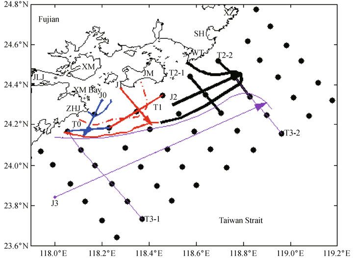
288                                                    Front. Earth Sci. 2013, 7(3): 282–294

      Fig. 6 Jet structures (curves) of velocity fields in the 2 m layer. Circles represent the velocities at the stations. Asterisks represent
      velocities by interpolation. (a)-(f) are for transects of T0, T1, T2-1, T2-2, T3-1 and T3-2, respectively.

flowing southwestward or southeastward. Third, J3 blocks                     model, verified by cruise data in the Delaware Bay,
J0 and J1 for running further offshore.                                     indicates that the inelastic collision between the terrestrial
                                                                            DOM molecules and dissolved salt ions in seawater is a
                                                                            decisive dynamic mechanism for the rapid loss of
4 MODIS observations of JRP and the                                         terrestrial DOM. In this paper, we apply the model to our
dynamic mechanism                                                           survey area. The terrestrial DOM distribution model is
                                                                            given as follows:
4.1   Spatial distribution of turbidity                                                 2                                 3

                                                                                                         0

High concentrations of particulate matter cause water to                                                     !
                                                                               n1 ðxÞ ¼ 4n1 ð0Þ þ 12 n2 ðxÞe 11 x= u dx5e –  11 x= u ,

                                                                                                     u
appear cloudy due to the absorption and scattering of light.                                                 x
The cloudiness of water is operationally measured as the                                                                                         (11)
amount of light transmitted. This quantity is termed
turbidity and reported in nephelometric turbidity units                     where n1 and n2 are the numbers of DOM and sodium
(NTU) (Libes, 2009). Suspended particulate matter is                        chloride molecules in a unit volume, respectively,  is the
mainly from phytoplankton and suspended sediment. The                       probability of inelastic collision between the DOM
former is the main source for open sea, while the latter for                molecules and the charged salt ions,      u is a mean flow
offshore waters (Huang et al., 2008).                                       velocity, x is the distance between the point on the x-
   Figure 7 shows the spatial distribution of the turbidity                 axis along the flow direction and the origin one with x
reanalyzed from the MODIS data on June 28, 2010 during                      = 0 km,  11 ¼ 421 ðπkT =m1 Þ1=2 ,
                                                                                                                 12 ¼ 2212 ð2πkT =m1 Þ1=2
the period of the summer cruise. In general, the turbidity in                ð1 þ m1 =m2 Þ , 1 is the particle size of DOM molecule,
                                                                                           1=2

the nearshore water is higher than that in the open sea. The                12 is a sum of the particle size of DOM and the radius of
turbidity in the open sea is more uniformly distributed,                    sodium chloride, m1 and m2 are their masses, k is the
with the turbidity less than 0.5 NTU. Seawater with high                    Boltzmann constant, and T is absolute temperature. Here
turbidity near the Xiamen Bay mouth flows northeastward                      n1 depends on the turbidity, and n2 on the salinity, n1(0) is
and southwestward at the same time. Furthermore, there is                   an initial value of n1.
also a stream of seawater with the high turbidity off Weitou                   In this paper, we choose the axis of high turbidity as the
flowing northeastward.                                                       x-axis, which is shown as a black curve with an origin at
                                                                            the black point O in Fig. 7. In order to determine the
4.2   Statistic-thermodynamical model                                       salinity-related parameter n2, we use a curve fitting method
                                                                            to establish a function of the salinity versus the distance
Based on the molecular collision theory in thermody-                        along x-axis. We choose 11 data points on x-axis for curve
namics and statistical physics, Zheng et al. (2008)                         fitting, which are stations X50, X41, X31, one point on
developed the terrestrial DOM distribution model. The                       connecting line of X21 and X22, and other seven points on
Daifeng WANG et al. Jet-like Jiulongjiang River plume discharging into the west Taiwan Strait 289
Fig. 7 Turbidity distribution derived from the MODIS observation on June 28, 2010. The black curve represents the axis of high
turbidity. Point O is chosen as the origin. SH, WT, JM, XM, and ZHJ represent Shenhu, Weitou, Jinmen, Xiamen, and Zhenhaijiao,
respectively.
x-axis. The salinity values of the first three points are taken
from cruise observations, and the other points are
calculated by Kriging interpolation.
As shown in Fig. 8, we fit salinity distribution with a
linear function, n2 ¼ b1 x þ b2 in which b1= 0.08 and b2=
28.08. And the correlation coefficient is 0.91 (significant at
the 95% level of confidence).
Substituting the linear function of n2 into Eq. (11) yields
b1
u
n1 ðxÞ ¼ n1 ð0Þ – 12 – b2 e – 11x= u Fig. 8 Salinity data fitting. Circles represent salinity at the
11 11 stations. Square represents salinity by interpolation.
12 b1
u
– b1 x þ b2 – : (12)
11
11 between the normalized mean turbidity data and the model
curve of 100 NTU reaches 0.96 (significant at the 95%
The normalized form of n1(x), i.e., n1 ðxÞ=n1 ð0Þ, is level of confidence).
defined as the turbidity index, and then its distribution Based on the above results, we can conclude that the
derived from Eq. (12) along x-axis is given as curves inelastic collision between the terrestrial DOM molecules
shown in Fig. 9. The parameters are reasonably taken as and dissolved salt ions may cause the molecules to adhere
follows: T = 293 K; m1= 1000 Da and m2 = 58.44 Da; to each other and form large size molecule groups; when
2 ¼ 2 10 – 4 m (Zheng et al., 2008); n1(0) is marked in the size grows large enough, the groups may sink toward
Fig. 9;
u is approximate to 0.5 m/s in the study area; ¼ the sea floor while changing their optic effect. The above
0:5 and k ¼ 1:38065 10 – 23 J=K. process is a decisive dynamic mechanism causing the loss
We use a four-point average method to calculate the of the terrestrial DOM in coastal seawater. In other words,
mean turbidity from the MODIS reanalyzed data. The four it is the salinity at a macro-scale which is a decisive factor
points are four resolution cells surrounding a position at that leads to the decrease of turbidity in coastal waters in
which the salinity data are taken. Comparison of the our study area. Theoretically, terrestrial DOM from the
normalized mean turbidity data with the DOM distribution Jiulongjiang River can reflect the path of the JRP.
model is shown in Fig. 9. The correlation coefficient Therefore, we can use the seawater turbidity as another290 Front. Earth Sci. 2013, 7(3): 282–294
turbidity data provides a clear signal of the high-turbidity
JRP. On the basis of the turbidity data from 2003 to 2011,
we can obtain a turbidity distribution image (Fig. 10)
which distinctly shows the presence of jets formed by the
Xiamen JRP and JinWei JRP on June 28, 2010 (Fig. 7).
This indicates that the jets developed by Xiamen JRP and
JinWei JRP as those on June 28 are not fortuitous
phenomena.
The natural indicator for freshwater plume in the coastal
ocean is salinity, but salinity cannot be remotely sensed at
useful spatial scales. Instead, turbidity can be another
indicator used to track the behavior of river plumes in the
coastal ocean. Comparing Fig. 2 with Fig. 7, one can see
that the general spreading trends for the JRP are north-
eastward and southwestward, but there exists some
difference between the in-situ salinity distribution and
Fig. 9 Turbidity index distribution along the x-axis derived from the turbidity distribution.
the DOM distribution model (curves). The basic points and error The elementary reasons follow. Firstly, the sources
bars are derived from the normalized MODIS turbidity by n1(0) on affecting the optical property of seawater are multiple
June 28, 2010. Three curves represent three cases of n1(0), nearshore, such as local resuspended sediment and the
including 50 NTU, 100 NTU and 500 NTU. bank erosion. So, strictly speaking, the factors that
determine the value of turbidity may be not just the
indicator for analysis of river plumes such as the JRP (Shi Jiulongjiang River. Secondly, the transport of terrestrial
and Wang, 2009). Figure 7 clearly shows the status of the DOM is complicated. Besides the inelastic collision
jets formed by the JRP on June 28, 2010. Meanwhile, the between the DOM molecules and dissolved salt ions,
signal of coastal upwelling off Xiangzhi-Weitou charac- photo-oxidation, mixing process, and bacterial degradation
terizes a lower turbidity in Fig. 7 as compared to the are also described as the mechanisms for the removal of
turbidity of JRP. terrestrial DOM (Wang et. al., 2004). So in the coastal area
the river runoff is the most important factor that influences
salinity, and as a tracer for river plume, salinity can display
5 Discussion more detailed patterns in comparison with turbidity.
5.1 Plume indicators 5.2 Four extension patterns for JRP
From the above study, we see that the MODIS reanalyzed The ability to apply turbidity to map plumes allows
Fig. 10 MODIS reanalyzed turbidity distribution displaying the status of jets formed by the JRP as Fig. 7 on August 29, 2003. SH, WT,
JM, XM, and ZHJ represent Shenhu, Weitou, Jinmen, Xiamen, and Zhenhaijiao, respectively.Daifeng WANG et al. Jet-like Jiulongjiang River plume discharging into the west Taiwan Strait 291
analysis of spatial patterns of the Jiulongjiang River and 5.3 Theoretical approximation
helps to further description and understanding of the JRP.
Due to the bio-optical, physical, and environmental In Section 3.2.1, we adopt the theory of a 2D jet (Kundu,
complexities, it is not every day we can get the satellite- 1990) as a physics model, which is used for interpretation
derived turbidity data on the study area, and not all of the of cruise observations. The 2D jet theory is derived based
distributions of turbidity can clearly display the signal of on the momentum balance between advection and lateral
JRP. viscosity. In the coastal ocean, however, there is a
In view of the turbidity distribution images on the days possibility for strong coastal currents to destroy such
with distinct JRP signals from the year of 2003 to 2010, momentum balance and modify the jet. In our case, from
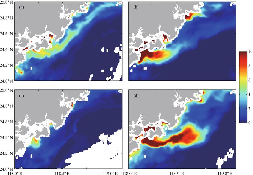
there are mainly four types of extending patterns for the Figs. 2 and 5, one can see that in an area near the Xiamen
JRP. First, going northward along the coastline (Figs. 11(a) Bay mouth, the diluted water plume patterns are indeed
and 12(a)) with the highest occurrence probability of 51%. close to the theoretical 2D jet. Beyond this area, the plume
Second, extending northeastward and southwestward at axes have remarkable turning, indicating the forcing of
the same time (Figs. 11(b) and 12(b)), i.e., it is a bi- coastal currents, but the plume structure still keeps a
directional plume with the second largest occurrence similarity to the 2D jet model. Thus, in our case, the 2D jet
probability of 20%. Third, just spreading out near the model is a rough approximation for interpretation of cruise
Xiamen Bay mouth (Figs. 11(c) and 12(c)) with 19% observations.
occurrence probability. The last but not the least , flowing Due to lack of current velocity data, we use the cruise-
northeastward offshore (Figs. 11(d) and 12(d)) with 10% measured density field to inverse the x-component of
occurrence probability. Figures 11 and 12 show the velocity u(y) using Eq. (10), t ¼ – αuðyÞ, where α is
representative images and average images for the four assumed to be a constant. Equation (10) is derived from the
patterns, respectively. continuity equation in the form of
Fig. 11 Turbidity representative distributions for the four extension patterns of JRP. (a)–(d) are those on August 17 of 2010, July 26 of
2011, July 16 of 2005 and August 28 of 2003, respectively, with corresponding occurrence probabilities as follow: 51%, 20%, 19% and
10%.292 Front. Earth Sci. 2013, 7(3): 282–294
Fig. 12 Average distributions of turbidity for the four extension patterns of JRP. (a)–(d) are those going northward along the coastline,
extending northeastward and southwestward at the same time, just spreading out near the Xiamen Bay mouth and flowing northeastward
offshore, respectively.
∂ northeastward into the survey area in the form of jet J3,
t ¼ – uðyÞ: (13)
∂x with the jet axis at an angle of 9° to the direction of the
coastline, whose intensity is the strongest as compared to
In general, ρ is a continuous function of x, assuming α other jets.
(=∂=∂x) to be a constant implies to take a linear After entering into the west Taiwan Strait, the Xiamen
approximation of ρ(x). JRP and JinWei JRP both take the shape of plume water
with fronts. The maximum width of the JRP coverage is
6 Summary about 31.5 km, and the length is about 86.3 km in the 2 m
layer. The isohalines are dense in the interaction zones of
We analyze the JRP based on the jet theory and the cruise the jets and form salinity fronts with the salinity gradient
observations carried out from June 28 to 30, 2010 in the up to 0.365/km.
west Taiwan Strait. The results indicate that in the 2 m In the 2 m layer, to some degree, the jets outside the
layer, the JRP flows into the adjacent water through Xiamen Bay are blocked by the strong jet J3, without
Xiamen Bay in the form of jets J0 and J1 in the flowing further offshore. The collision between J2 and J3
southwestward and southeastward directions with angles prevents the JinWei JRP from spreading southwestward or
of 151° and 90° to the direction of the coastline, southeastward. The JinWei JRP, dragged by jet J3, extends
respectively. Meanwhile, the JRP enters into the west northeastward. Vertically, jet J0 has an influence depth
Taiwan Strait through the channel between Jinmen and from 2 to 7 m, with a shorter axis length in its 7 m layer. It
Weitou in the form of jet J2 whose axis directs north- also shows that the JRP has an impact depth of less than
eastward with an angle of 9° to the direction of the 10 m.
coastline. Driven by the summer southwesterly monsoon, Using the terrestrial DOM distribution model developed
Dongshan low temperature and high salinity water runs by Zheng et al. (2008), we analyzed the DOM degradationDaifeng WANG et al. Jet-like Jiulongjiang River plume discharging into the west Taiwan Strait 293
in the study area. The correlation coefficient of the M (2009a). Inter annual variability of summer coastal upwelling in
theoretical model to the MODIS turbidity data is 0.96 the Taiwan Strait. Cont Shelf Res, 29(2): 479–484
(significant at the 95% level of confidence). The results Hong H S, Zheng Q A, Hu J Y, Chen Z Z, Li C Y, Jiang Y W, Wan Z W
indicate that the inelastic collision between the terrestrial (2009b). Three-dimensional structure of a low salinity tongue in the
DOM molecules and dissolved salt ions in seawater is a southern Taiwan Strait observed in the summer of 2005. Acta
decisive dynamic mechanism to cause the loss of terrestrial Oceanol Sin, 28(4): 1–7
DOM in coastal regions. At the macro-scale, the salinity is Huang Y C, LI Y, Shao H, Li Y H (2008). Seasonal variations of sea
a decisive factor for the diminishing of turbidity in the surface temperature, chlorophyll a and turbidity in Beibu Gulf,
study area. Thus we can utilize the turbidity as an indicator MODIS imagery study. Journal of Xiamen University (Natural
to study the extension patterns of the JRP. For example, in Science), 47(6): 856–863
the MODIS turbidity distribution image on June 28, 2010, Kim H C, Yamaguchi H, Yoo S, Zhu J R, Okamura K, Kiyomoto Y,
one can clearly see the status of the jets formed by the JRP. Tanaka K, Kim S W, Park T, Oh IS, Ishizaka J (2009). Distribution of
According to the MODIS reanalyzed turbidity data, Changjiang diluted water detected by satellite chlorophyll a and its
there are mainly four spatial extending patterns for the JRP, interannual variation during 1998–2007. J Oceanogr, 65(1): 129–135
which are listed from the highest occurrence probability to Kundu P K (1990). Fluid Mechanics. San Diego: Academic Press, 478–
the lowest one. These include running northward along the 481
coastline with the occurrence probability of 51%, a bi- Libes S (2009). Introduction to Marine Biogeochemistry. San Diego:
directional plume with branches spreading northeastward Academic Press, 208
and southwestward at the same time with the occurrence Lie H J, Cho C H, Lee J H, Lee S (2003). Structure and eastward
probability of 20%, just extending out near the Xiamen extension of the Changjiang River plume in the East China Sea. J
Bay mouth with 19% occurrence probability and flowing Geophys Res, 108(C3 3077): 22, 1–14
northeastward offshore with 13% occurrence probability. Liu Y G, MacCready P, Hickey B M (2009a). Columbia River plume
patterns in summer 2004 as revealed by a hindcast coastal ocean
Acknowledgements This work was jointly supported by the National Basic circulation model. Geophys Res Let, 36: L02601
Research Program of China (No. 2009CB21208) and the National Natural Liu Y G, MacCready P, Hickey B M, Dever E P, Kosro P M, Banas N S
Science Foundation of China (Grant Nos. 41276006, 41121091 and
(2009b). Evaluation of a coastal ocean circulation model for the
40810069004). The authors would like to express their appreciation to the
crew of R/V Yanping 2 and all of the cruise participants for help with the field Columbia River plume in 2004. J Geophys Res, 114(C2): C00B4
work. We thank Ms. Yonghong Li for providing the MODIS satellite data, Liu Y G, Weisberg R H (2007). Ocean currents and sea surface heights
Mr. Zhenyu Sun and Ms. Jia Zhu for their insightful suggestions. Zheng also estimated across the West Florida Shelf. J Phys Oceanogr, 37(6):
appreciates the financial support by a Key Program from the State 1697–1713
Administration of Foreign Experts Affairs of China. We are grateful to two
Luo Z B, Pan W R, Li L, Zhang G R (2011). Salinity fronts at
anonymous reviewers for their valuable suggestions and comments for
improving the manuscript. Jiulongjiang Estuary. IEEE Remote Sensing, Environment and
Transportation Engineering (RSETE), 3449–3454
Luo Z B, Pan W R, Li L, Zhang G R (2012). The study on three-
References dimensional numerical model and fronts of the Jiulong Estuary and
the Xiamen Bay. Acta Oceanol Sin, 31(4): 55–64
Chao S Y, Boicourt W C (1986). Onset of estuarine plumes. J Phys MacCready P, Banas N S, Hickey B M, Dever E P, Liu Y G (2009). A
Oceanogr, 16(12): 2137–2149 model study of tide- and wind-induced mixing in the Columbia River
Chen H, Hu J Y, Pan W R, Zeng G N, Chen Z Z, He Z G, Zhang C Y, Li Estuary and plume. Cont Shelf Res, 29(1): 278–291
H (2002). Underway measurement of sea surface temperature and Mao H L, Gan Z J, Lan S F (1963). A preliminary study of the Yangtze
salinity in the Taiwan Straits in August, 1999. Marine Science diluted water and its mixing processing. Oceanologia ET Limnologia
Bulletin, 4(1): 11–18 Sinica, 5(3): 183–206 (in Chinese)
Chen J Q, Fu Z L, Li F X (1982). Study of upwelling in Minnan-Taiwan Ortner P B, Lee T N, Milne P J, Zika R G, Clarke M E, Podesta G P,
Bank. J Oceanogr Taiwan, 2(1): 5–13 (in Chinese) Swart P K, Tester P A, Atkinson L P, Johnson W R (1995).
Chen X H, Hu J Y, Pi Q L, Liu G P, Chen Z Z (2009). Densely underway Mississippi River flood water that reached the Gulf Stream. J
measurement of surface temperature and salinity in Xiamen- Geophys Res, 100(C7): 13595–13601
Quanzhou near-shore area. Advances in Earth Science, 24(6): 629– Rong Z R, Li M (2012). Tidal effects on the bulge region of Changjiang
635 (in Chinese) River plume. Estuar Coast Shelf Sci, 97(20): 149–160
Guo W D, Yang L Y, Hong H S, Stedmon C A, Wang F L, Xu J, Xie Y Y Schiller R V, Kourafalou V H, Hogan P, Walker N D (2011). The
(2011). Assessing the dynamics of chromophoric dissolved organic dynamics of the Mississippi River plume–impact of topography,
matter in a subtropical estuary using parallel factor analysis. Mar wind and offshore forcing on the fate of plume waters. J Geophys
Chem, 124(1–4): 125–133 Res, 116(C6): C06029
Hickey B, Geier S, Kachel N, MacFadyen A (2005). A bi-directional Shi W, Wang M H (2009). Satellite observations of flood-driven
river plume: the Columbia in summer. Cont Shelf Res, 25(14): 1631– Mississippi River Plume in the spring of 2008. Geophys Res Lett, 36
1656 (7): L07607
Hong H S, Zhang C Y, Shang S L, Huang B Q, Li Y H, Li X D, Zhang S Wang X C, Chen R F, Gardner G B (2004). Sources and transport of294 Front. Earth Sci. 2013, 7(3): 282–294
dissolved and particulate organic carbon in the Mississippi River Sciences, Xiamen University, China. Her current research interests
estuary and adjacent coastal waters of the northern Gulf of Mexico. focus on river plume. E-mail: dfengw@xmu.edu.cn
Mar Chem, 89(1–4): 241–256
Wu H, Zhu J R, Shen J, Wang H (2011). Tidal modulation on the
Changjiang River plume in summer. J Geophys Res, 116(C8): Dr. Quan’an Zheng is a Senior Research Scientist of the Department
C08017 of Atmospheric and Oceanic Science, University of Maryland, USA,
Zhang C Y, Hong H S, Hu C M, Shang S L (2011). Evolution of a coastal and a Guest Chair Professor of Xiamen University, China. His
upwelling event during summer 2004 in the southern Taiwan Strait. research interests are ocean remote sensing (including physics, data
Acta Oceanol Sin, 30(1): 1–6 interpretation, applications, and laboratory simulation), ocean sur-
Zhang Y H, Wang W Q, Huang Z Q (1999). Salinity fronts and chemical face processes (including wind friction, wave spectra, skin layer
behavior of nutrient in Jiulongjiang Estuary. Marine Environmental physics, and surfactant effects), upper ocean dynamics (including
Science, 18(4): 1–7 (in Chinese) internal wave dynamics and ocean-atmospheric coupling), meso-
Zheng Q A, Chen Q, Zhao H H, Shi J X, Cao Y, Wang D (2008). A scale ocean dynamics, and solitary waves in the atmosphere and
statistic-thermodynamic model for the DOM degradation in the ocean. E-mail: quanan@atmos.umd.edu. Website: http://www.
estuary. Geophys Res Lett, 35(6): L06604 atmos.umd.edu/~quanan/
Zheng Q A, Clemente-Colon P, Yan X H, Liu W T (2004). Satellite
synthetic aperture radar detection of Delaware Bay plumes: Jet-like
feature analysis. J Geophys Res, 109(C3): C03031 Dr. Jianyu Hu obtained his Ph.D degree (2001) in physical
oceanography from Tohoku University of Japan and Ph.D degree
(2002) in environmental science from Xiamen University of China.
AUTHOR BIOGRAPHIES He is now a professor in State Key Laboratory of Marine
Environmental Science and Department of Physical Oceanography
at Xiamen University, focusing on the study of regional environ-
Daifeng Wang is a Ph.D Candidate in the College of Ocean and Earth mental oceanography.You can also read