A Brief Analysis of the Triangle Method and a Proposal for its Operational Implementation
←
→
Page content transcription
If your browser does not render page correctly, please read the page content below
remote sensing
Letter
A Brief Analysis of the Triangle Method and a
Proposal for its Operational Implementation
Toby N. Carlson
 Department of Meteorology, Penn State University, University Park, PA 16802, USA; tnc@psu.edu

 Received: 16 October 2020; Accepted: 19 November 2020; Published: 22 November 2020

 Abstract: The well-known triangle method in optical/thermal remote sensing, its construction,
 uncertainties, and the significance of its products are first discussed. These topics are then followed
 by an outline of how the method can be implemented operationally for practical use, including a
 suggestion for constructing a dynamic crop moisture index.

 Keywords: triangle method; remote sensing; soil water content; evapotranspiration

1. Background
      Despite its increasing popularity, evidenced by the plethora of papers on the subject, the triangle
method in optical/thermal remote sensing remains an unclear subject, so far lacking any consensus on
how to construct the triangle or on a mathematical formalism. Lacking also is a full appreciation for its
inherent limitations, the nature of its derivative products, and a clear focus on how it might be used
operationally. To briefly summarize, the triangle method allows one to estimate surface soil water
content and evapotranspiration fraction EF (here defined as the ratio of transpiration T to net radiation
Rn) from remotely sensed optical and thermal measurements. The triangle’s greatest advantage is its
mathematical and geometric simplicity and that it requires no ancillary surface or atmospheric data
and no detailed land surface model.
      In all versions of the triangle method, some sort of mathematical formalism serves as an
interface with the input measurements to yield the output: EF and a surface moisture parameter Mo.
Input parameters are surface radiant temperature (Tir) and a vegetation index (e.g., NDVI), from which
fractional vegetation cover (Fr) is determined. Mo, the surface moisture parameter, is called the surface
moisture availability and is loosely defined as the ratio of soil water content to that at field capacity.
      Considerable discussion of the triangle method and its application exists in several recent
papers (de Tomas et al. [1], Rasmussen et al. [2], Carlson and Petropoulos [3], Silva-Fuzzo et al. [4],
Kasim et al. [5], Petropoulos et al. [6]). Many other papers published over the past 25 years have dealt
with this subject. In the interest of brevity and to confine the subject to the narrow topic of the triangle,
this paper will eschew a lengthy literature review but refer mainly to those papers published on this
subject during the past few years. The purpose of this paper is to present the method concisely and
to point the way toward its operational implementation, for example for use in the European Space
Agency’s Sentinel-3 program [6]. Accordingly, the paper will just briefly outline the mathematical and
conceptual basis for the triangle method, discuss some of its inherent uncertainties, precisely describe
the nature of its products, and, finally, present steps toward a realization of the triangle method as an
operational tool for routinely assessing soil moisture status.

2. Construction of the Triangle
     When surface infrared temperature Tir is plotted against vegetation index NDVI or Fr one often
finds a triangular patten in the pixel envelope, such as is illustrated in Figure 1. This configuration is

Remote Sens. 2020, 12, 3832; doi:10.3390/rs12223832                       www.mdpi.com/journal/remotesensing
Remote Sens. 2020, 12, x 2 of 9
When surface infrared temperature Tir is plotted against vegetation index NDVI or Fr one often
Remote Sens. 2020, 12, 3832 2 of 9
finds a triangular patten in the pixel envelope, such as is illustrated in Figure 1. This configuration is
most apparent under the following conditions: the image contains a sufficiently large number of
pixels
most with at
apparent leastthesome
under containing
following both the
conditions: vegetation and bare
image contains soil, the large
a sufficiently surface is not
number highly
of pixels
inhomogeneous
with at least some(e.g., a forestboth
containing aside field of short
vegetation andgrass), thethe
bare soil, surface does
surface is not
notslope
highlybyinhomogeneous
more than about
10%,a forest
(e.g., and standing
aside field water andgrass),
of short cloud theare surface
removed. Itsnot
does triangular
slope byshape represents
more than the fact
about 10%, andthat, while
standing
Tir can
water vary
and considerably
cloud are removed.over bare
Its soil, depending
triangular shape onrepresents
soil wetness theand composition,
fact that, whileitTirdoes
cannotvary
very
spatially byover
considerably morebare than a very
soil, small amount
depending over vegetation
on soil wetness (at least itnodoes
and composition, greater thanspatially
not very the errorbyin
measuring
more than a Tir).
very While individual
small amount overleaves can experience
vegetation (at least anorange of temperatures
greater than the errorfrom strong sunlight
in measuring Tir).
to shade,
While it is this
individual author’s
leaves experiencea range
can experience that large clumps of dense
of temperatures vegetation
from strong on scales
sunlight much
to shade, it islarger
this
than individual
author’s experience leaves remains
that large uniformly
clumps of denseabout 1 °C or on
vegetation so above air temperature
scales much larger thanatindividual
least untilleaves
severe
wiltinguniformly
remains occurs. The aboutlatter
1 ◦ Cobservation
or so above air is temperature
consistent with theuntil
at least surface
severe sensible
wiltingheat fluxThe
occurs. H latter
being
typically small
observation over vegetation.
is consistent with theThus,
surface thesensible
triangleheat
shape
fluxisHdetermined not by
being typically the vegetation
small but by
over vegetation.
the bare
Thus, soil around
the triangle shapetheisplants.
determined not by the vegetation but by the bare soil around the plants.
Figure
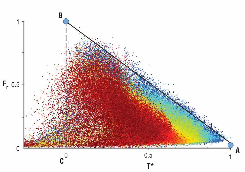
Figure 1. 1. Triangle
Triangle for for satellite
satellite images
images over over soybean
soybean fields fields in (Silva-Fuzzo
in Brazil Brazil (Silva-Fuzzo
et al. [4]).etScaled
al. [4]). Scaled
surface
surface radiant temperature (T*) is plotted along the horizontal axes and fractional vegetation cover
radiant temperature (T*) is plotted along the horizontal axes and fractional vegetation cover (Fr) is
(Fr) is along
plotted plottedthealong the axes.
vertical vertical
Theaxes.
warm The warm
edge edge is denoted
is denoted by the red
by the slanting slanting
lines red
andlines andedge
the cold the cold
is
edge by
shown is shown
the bluebylines
the along
blue lines along axes.
the vertical the vertical
Triangle axes. Trianglewere
boundaries boundaries were all
all determined determined
subjectively.
subjectively.
Given the appearance of a triangular shape, the vertical axis can be expressed either as the
Givendifference
normalized the appearance
vegetationof aindex
triangular
(NDVI) shape, the vertical
or fractional axis can
vegetation be (Fr)
cover expressed
and theeither as the
horizontal
asnormalized difference vegetation index (NDVI) or fractional vegetation cover (Fr) and the horizontal
a scaled temperature T*, to be defined below. Two anchor points, A and B, are defined in Figure 2.
as a scaled
These points temperature
correspond toT*,thetolower
be defined below.
right-hand Two(A)
vertex anchor points,
where Tir is A and B, are over
a maximum defined in surface,
a bare Figure 2.
= 0, called
FrThese points correspond to the lower right-hand vertex (A) where Tir is a maximum over a bare
Tmax, the vegetation index being defined as NDVIo. The upper vertex (B) corresponds
tosurface,
dense vegetation, Fr = Tmax,
Fr = 0, called 1.0, wherethe NDVI
vegetation indexasbeing
is defined NDVIs defined
and Tirasis NDVIo. The the
called Tmin, upper vertex (B)
temperature
corresponds to dense vegetation, Fr = 1.0, where NDVI is defined as NDVIs and Tir is called Tmin,
over dense vegetation, Tmin is also representative of a minimum temperature in the image when all
the temperature over dense vegetation, Tmin is also representative of a minimum temperature in the
extraneous pixels are removed; the tail of pixels at the lower left-hand corner of Figure 2 are likely due
toimage
cloudwhen all extraneous
or standing pixelsthese
water. Given are removed;
endpoints, theatail of pixels
vertical coldatedge
the lower left-hand
is drawn down corner of Figure
to the soil line
2 are likely due to cloud or standing water. Given these endpoints, a vertical cold edge is drawn down
from points B to C, defining the boundaries of a right triangle and thereby enclosing almost all the
pixels within the triangle. Tir is replaced by the temperature T*, which is scaled between Tmax and
Tmin (Equation (2)) and which varies from zero to one. Similarly, NDVI is scaled from its minimum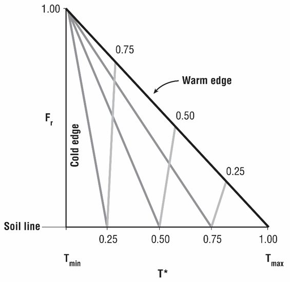
Remote Sens. 2020, 12, x 3 of 9
to the soil line from points B to C, defining the boundaries of a right triangle and thereby enclosing
almostSens.
Remote all 2020,
the pixels
12, 3832within the triangle. Tir is replaced by the temperature T*, which is scaled between 3 of 9
Tmax and Tmin (Equation (2)) and which varies from zero to one. Similarly, NDVI is scaled from its
minimum to maximum value and converted to Fr with a simple algorithm (Equation (1)). The
segment
to maximumB–C,value
the cold
andedge, forms atoright
converted triangle
Fr with and bounds
a simple algorithmalmost all the pixels
(Equation on its
(1)). The warm side.
segment B–C,
Although no fundamental reason exists for the verticality of the cold edge, the data almost always
the cold edge, forms a right triangle and bounds almost all the pixels on its warm side. Although no
support this assumption,
fundamental reason existswhich allows
for the for a more
verticality of thesimplified
cold edge,geometry
the datathan a slanting
almost alwaysone.
support this
assumption, which allows for a more simplified geometry than a slanting one.
Figure 2.
Figure 2. Triangle
Triangle created
createdfrom
fromaaSentinel-3
Sentinel-3image
imagemademadeover
over Spain
Spain at at 1 km
1 km resolution
resolution (axes
(axes labeled
labeled as
as fractional vegetation cover and scaled infrared surface temperature, respectively Fr and T*). Small
fractional vegetation cover and scaled infrared surface temperature, respectively Fr and T*). Small circles
circles marked
marked A and BAdenote
and Bthedenote
anchorthe anchor
points points
of the of theSloping
triangle. triangle.
lineSloping
betweenline between
A and A and B
B corresponds
corresponds
to to the warmfixed
the warm edge—here edge—here fixed by inspection—and
by inspection—and thebetween
the vertical line vertical Bline
andbetween
C is the Bcold
andedge,
C is
the cold edge, also determined visually. (Image courtesy of George Petropoulos).
also determined visually. (Image courtesy of George Petropoulos).
In
In Figures
Figures 11 andand 2,
2, the
the warm
warm and and cold
cold edges
edges were
were constructed
constructed by by eye.
eye. Alternately,
Alternately, one one can
can
construct
construct the warm edge more objectively. Following Tang et al. [7], the Fr axis is sliced into small
the warm edge more objectively. Following Tang et al. [7], the Fr axis is sliced into small
segments
segments (e.g.,
(e.g., 0.1
0.1 wide)
wide) and
and aa warm
warm edge
edge isis estimated
estimated for for each
each slice
slice atat the
the point
point where,
where, proceeding
proceeding
from
from the cold edge, a threshold value (e.g., 99%) of the pixels in that slice has been counted.
the cold edge, a threshold value (e.g., 99%) of the pixels in that slice has been counted. OnceOnce all
all
threshold
threshold points are made over the full range of Fr, the warm edge is constructed as the least squares
points are made over the full range of Fr, the warm edge is constructed as the least squares
straight line through
straight line through these
these points
pointsextending
extendingfrom fromthe thebase
baseofofthethetriangle,
triangle,thethe soil
soil line
line at at point
point A, A,
to
to where it meets the vertical axis, the cold edge, at point B. This procedure is referred
where it meets the vertical axis, the cold edge, at point B. This procedure is referred to by de Tomas to by de Tomas
et
et al.
al. [1]
[1] as
as the
the ‘Tang
‘Tang dry
dry edge
edge algorithm’.
algorithm’.
Scaled
Scaled variables
variables (T*)
(T*) and
and Fr
Fr are
are calculated
calculated as as follows:
follows:
(1)
FrFr==((NDVI
((NDVI−– NDVIo)/(NDVIs
NDVIo)/(NDVIs−– NDVIo))
NDVIo))22 (1)
T* = (Tir – Tmin)/(Tmax – Tmin) (2)
T* = (Tir − Tmin)/(Tmax − Tmin) (2)
from which the important moisture variables Mo and EF are calculated. T* is sometimes referred to
as thewhich
from ‘temperature-dryness index’.variables
the important moisture For a right
Motriangle
and EF are calculated. T* is sometimes referred to as
the ‘temperature-dryness index’. For a right triangle
Mo = 1-T* (pixel)/(1-Fr) (3)
EF== 1EF
Mo (1-Fr)
−sT* + EFveg−*Fr
(pixel)/(1 Fr) (4)
(3)
where Mo pertains only to the bare soilEF =surface
EFs (1 and
− Fr)EFveg is the
+ EFveg *Frtranspiration fraction for vegetation.
(4)
The latter is assumed to be at potential and therefore it is equal to 1.0.
where Mo pertains only to the bare soil surface and EFveg is the transpiration fraction for vegetation.
3. Significance
The of theto
latter is assumed Triangle Bordersand therefore it is equal to 1.0.
be at potential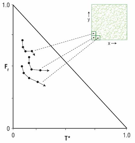
Remote Sens. 2020, 12, 3832 4 of 9
Remote Sens. 2020, 12, x 4 of 9
3. Significance of the Triangle Borders
As shown in Figures 1 and 2, the triangle typically exhibits reasonably well-defined borders,
particularly
As shown along the bottom
in Figures 1 and of 2,
thethe triangle
triangle (the soil line)exhibits
typically and its reasonably
sloping warm side, the warm
well-defined (or
borders,
dry) edge. along
particularly Such thesharp edges
bottom of in
thenature
trianglesignify
(the soillimits of some
line) and kind: warm
its sloping in this case
side, thethe
warmlimit
(orofdry)
no
vegetation
edge. at its base
Such sharp edgesand the limit
in nature of soil
signify dryness
limits along
of some its warm
kind: in thisedge. A cold
case the limitedge,
of nosignifying
vegetationthe at
limit
its base ofand
maximum
the limitwetness (field capacity
of soil dryness along itsand warmpotential
edge. A evaporation), is often less
cold edge, signifying the well-defined,
limit of maximum as is
evident (field
wetness in Figure 2. and potential evaporation), is often less well-defined, as is evident in Figure 2.
capacity
Twoaspects
Two aspectsof ofthese
thesetriangles
trianglesare areobvious.
obvious.First,First,the
the choice
choiceof oftheir
theirwarm
warmand and cold
cold edges
edges can
can be
be
somewhat disputed,
somewhat disputed, and,and, second,
second, the the triangles
triangles sometimes
sometimes exhibitexhibit small
small areas
areas with
with fewfew oror no
no pixels,
pixels,
thereby obscuring
thereby obscuring somewhat
somewhat the the location
location of of these
these boundaries.
boundaries. These These gaps
gaps maymay occur,
occur, forfor example,
example,
becausepixels
because pixelsoverover bare,
bare, wetwetsoilssoils are relatively
are relatively uncommon
uncommon making making
the coldthe cold
edge edge particularly
particularly difficult
difficult
to locate.to locate.
Often, Often,
what what to
appears appears
be dense to be dense vegetation
vegetation actually actually exhibits openings
exhibits openings in the plant in the plant
canopy
canopy
so so that
that the upper thevertex
upperisvertex
absent is of
absent
pixels ofand
pixelstheand the resembles
figure figure resembles a trapezoid,
a trapezoid, a situation
a situation to be
to be addressed
addressed in Section
in Section 4. 4.
In these
In these types
types ofof analyses,
analyses, oneone assumes
assumes that that all
all the
the fields
fields internal
internal to to the
the triangle
triangle vary
vary linearly
linearly
across the
across the domain.
domain. ThisThis enables
enables oneone to to solve
solve forfor EF
EF and
and Mo Mo using
using just
just aa very
very fewfew simple
simple algebraic
algebraic
formulae. The
formulae. The solution
solution takes
takes the
the form
form of of the
the configuration
configuration of of EF
EF and
and Mo
Mo shown
shown in in Figure
Figure3.3. AsAs the
the
vertical and
vertical and horizontal
horizontal axes axes both
both vary
vary fromfrom 00 to to 1.0,
1.0, all
all triangles
triangles formed
formed withwith these
these equations
equations are are
mathematicallycongruent,
mathematically congruent, constituting
constituting a ‘universal’
a ‘universal’ triangle.triangle. The assumption
The assumption of linearity of islinearity
addressed is
addressed
in Section 4.in Section 4.
Figure 3.
Figure 3. Solutions
SolutionstotoEquations
Equations(3)(3)
and (4).(4).
and Isopleths of Mo
Isopleths of(lines sloping
Mo (lines upward
sloping to the left,
upward labeled
to the left,
below the
labeled figure)
below and EFand
the figure) (lines
EFsloping upwardupward
(lines sloping to the right,
to thelabeled to the right).
right, labeled to the right).
4. Uncertainties in the Triangle
4. Uncertainties in the Triangle
The triangle approach raises questions concerning the method of assigning its boundaries and the
The triangle approach raises questions concerning the method of assigning its boundaries and
accuracy of the various assumptions. These will now be addressed.
the accuracy of the various assumptions. These will now be addressed.
4.1. Errors Arising from the Choice of Anchor Points
4.1. Errors Arising from the Choice of Anchor Points
An obvious source of uncertainty is the choice of the anchor points that define the vertices of
An obvious source of uncertainty is the choice of the anchor points that define the vertices of the
the triangle, A and B in Figure 2. Both points are susceptible to the uncertainty of choice or to the
triangle, A and B in Figure 2. Both points are susceptible to the uncertainty of choice or to the
algorithm used to create it, such as a regression line. Some papers have addressed the issue of how
much error is engendered by an incorrect location of the warm edge, but this source of error needs toRemote Sens. 2020, 12, 3832 5 of 9
algorithm used to create it, such as a regression line. Some papers have addressed the issue of how
much error is engendered by an incorrect location of the warm edge, but this source of error needs to
be studied further. Gillies and Carlson [8] thought that it is possible that multiple warm edges might
occur in the same image. It seems quite likely that some error in fixing the warm edge can arise from
the fact that Tmax and Tmin may have different values within the triangle, the result of differing soil
and vegetation types in the image. Addressing uncertainty in choosing these anchor points is further
discussed in Section 5. As referred to above, the location of the cold edge is problematic because of the
irregular distribution of pixels on that side of the triangle. In practice, nature does not lend itself to
simple geometry, so it is necessary to adjust the segment B–C in Figure 2 to intercept the warm edge so
as to maintain a right triangle and still include most of the pixels within the triangle.
4.2. The Problem of Scale
Most of us who work with satellite or aircraft imagery believe the higher the resolution is the better.
Triangles certainly tend to degrade as the resolution decreases above about 1 km but appear highly
satisfactory in the Sentinel image (0.5–1.0 km resolution; Figure 2, see also Gillies and Carlson [8]) and
Landsat with its 30–120 resolution (Figure 1). However, extremely high resolution (pixels less than
several meters in size) can cause a problem due to small irregularities in the terrain (humps and furrows)
and local variations in leaf angles. Such local variations can distort the sun angles, causing significant
variations in incident solar flux from those on a horizontal surface, thereby introducing anomalously
warm or cold pixels. In such imagery, the triangle edges tend to be fuzzy and less resolvable and so
should be composited, as to yield sharper triangle boundaries.
4.3. Triangle or Trapeziod
Many papers on this subject refer to a trapezoid rather than a triangle (e.g., Babaeirian et al. [9]).
A trapezoid is just triangle truncated at the top, implying a space void of pixels below the projected
vertex. Using a full soil/vegetation/atmosphere/transfer (SVAT) model described by Carlson [10], it was
found that a variation of Mo with Tir occurs at full vegetation when the leaf area index (LAI) is not
very large (e.g., 3 or less), presumably because the vegetation canopy still exhibits gaps through which
radiance from the bare soil beneath can reach the radiometer. When LAI is raised well above 3 in these
simulations, the trapezoid collapses to a right triangle, suggesting that the true value of Fr is higher
than that originally selected for a full vegetation cover. De Tomas et al. [1] also found the same thing:
that the trapezoid reduced to a triangle when LAI was increased to amounts well above 3. Here the
full vegetation cover Fr = 1 is defined as that at the triangle’s upper vertex (point B in Figure 2), even if
no pixels appear just below it.
4.4. The Assumption of Linearity
A fundamental assumption in the triangle method is that all fields interior to the triangle
(or trapezoid) vary linearly. That assumption leads to the interior isopleths of Mo and EF shown in
Figure 3.
Solutions for these two variables generated from more complex models, such as the SVAT model
referred to in Carlson [10], show very similar nearly straight lines for Mo to those shown in this figure.
emanating from the upper vertex to the soil line. EF, on the other hand, is highly nonlinear. Carlson and
Petropoulos [3] show that on the average the differences with the linear model are generally less than
20%. Kasim et al. [5] also found close agreement between the fields of Mo and EF generated with the
model described above [10] and those represented in Figure 3. Very similar fields of EF to those in
Figure 3 are shown by de Tomas et al. [1].
While it might seem useful to determine more accurate values for Mo and EF with a more
mathematically complex formalism, it is not clear whether the large number of surface and atmospheric
and plant parameters necessary to initialize such models and the mathematical complexity facing theRemote Sens. 2020, 12, 3832 6 of 9
user in operating them would result in more accurate, practical, or cost effective solutions for Mo
and EF.
4.5. The Meaning of Mo and EF
Moisture availability Mo is generally equated to the soil water content as the fraction of field
capacity or a similar upper value (e.g., saturation). Little evidence exists for assuming a linear
relationship, although various studies demonstrate it to be highly correlated with soil water content,
albeit generally with low values of correlation, as in Kasim et al. [5].
One problem in equating Mo to soil water content is that comparisons with field measurements are
generally rather poor because in situ measurements are usually confined to the top 5 cm, whereas Tir
represents a soil skin temperature which is best correlated with water content within the top 1 cm
(Capehart and Carlson, [11]). Another problem with Mo is that the accuracy of thermal/optical methods
deteriorates with increasing Fr, completely losing any value as Fr approaches 1.0. Consequently,
Mo values are essentially valueless near the upper vertex of the triangle (Gillies and Carlson, [8];
Kasim et al. [5]). Conversely, agreement with ground measurements shows a much better correlation
when comparisons are limited to pixels with small amounts of vegetation Kasim et al. [5].
Evapotranspiration fraction EF is more useful than transpiration itself, which is highly transient.
Depending on its definition (as ET/Rn or ET/(Rn - G), where G is the ground heat flux), EF corresponds
approximately or exactly to the Bowen ratio which is defined as H/ET where H is the surface heat flux
and ET is the evapotranspiration. As the Bowen ratio is known to remain approximately constant
throughout most of the solar day, it can be used to calculate total water lost from the soil during the
day by multiplying EF by the total net radiation absorbed at the ground over the length of the solar day.
(Note that the ground heat flux G tends toward zero when averaged over a full 24 h.) Both Rasmussen
et al. [2] and de Tomas et al. [1], using the triangle method, mapped the value of φ (the modifier of the
Penman–Monteith evapotranspiration formula), which is essentially identical to EF.
5. Practical Considerations
5.1. Operational Implementation
It is hard to conceive at present that a fully operational system for a practical and systematic
implementation of the triangle could be accomplished without a human/machine synergy. The latter
is envisaged as the person, interacting with the computer by means of an electronic pen or cursor,
whose function would be to insert the two anchor points A and B on an image of pixels plotted in Tir
and NDVI space. This would be done according to steps summarized below and illustrated by the
image in Figure 2, the latter made over an agricultural site in Spain by Sentinel-3 (Petropoulos et al. [3]).
What follows is a roadmap on how this might be accomplished.
• Pixels contaminated by cloud or standing water are first removed. Elimination of these anomalies
is accomplished by realizing that the ratio of visible reflectance to Tir is much higher for cloud
pixels and the product of NDVI times Tir is much smaller for standing water than for most
natural surfaces.
• Remaining pixels are plotted by computer on orthogonal axes as values of Tir and NDVI, as in
Figure 2.
• With an electronic pen or cursor, the user inspects the image and visually marks with a dot on the
computer monitor the two anchor points, labeled A and B, as in Figure 2. These points correspond,
respectively, to Tmax and NDVIo (Fr = 0) and to Tmin and NDVIs (Fr = 1).
• Once points A and B are marked, the computer relabels the axes as Fr and T* (using Equations (1)
and (2)) and internally calculates Mo and EF (using Equations (3) and (4)).
• Having marked the two anchor points, the computer immediately draws the warm edge between
points A and B and the cold edge between B and C, where the line B–C is drawn vertically fromachieve a satisfactory and mutually consistent set of borders for the triangle.
• Anchor points A and B may need further adjustment in order to be compatible with the
overall pixel distribution and the warm edge. During this process of adjustment, the
triangle’s scaling and the internal values of Mo and EF are continually being recalculated.
Remote•Sens.When the
2020, 12, user is satisfied with the construction, all values of Mo and EF within the triangle
3832 7 of 9
are mapped to the surface area over which the image was made.
5.2. Athe warm edge
Dynamic Cropline to intersect
Moisture Index with the soil line. In so doing, vertical line B–C, the cold edge line,
should contain most of the pixels on its warm side.
• Frequent
The references
computer haves been
then constructs andmade in the
alternate literature
warm to a by
edge line crop moisture
first index,a many
determining of points
series of which
are virtual transforms of Mo (Jackson et al. [12]). Whether a variation of Mo or as
in slices of Fr from zero to one corresponding to a threshold percentage of pixels (e.g., 99%) asa two-dimensional
variable (Fr, T*)
described withinthe
above: the‘Tang
triangle, a crop(de
dry edge’ moisture
Tomas index currently represents a single number that
et al. [1]).
does not unambiguously prescribe a level of water stress. A clearer picture of water stress would be
• An alternate warm edge is constructed by a linear least squares fit to these points and the line
achieved by monitoring the changes in the stress parameter over time by including trajectories of
extended to the soil line and the vertical cold edge. The user would then have the option of
points within the triangle for fixed surface locations as represented by the three trajectories in Figure
adjusting the visual and analytical warm edges (by moving the anchor points A and B) to achieve
4.
a satisfactory and mutually consistent set of borders for the triangle.
Each of these three trajectories pertains to values of Mo and EF on five successive days
• Anchor points A and B may need further adjustment in order to be compatible with the overall
represented by the five dots (including the arrowhead) along the trajectories. Each trajectory pertains
pixel distribution and the warm edge. During this process of adjustment, the triangle’s scaling
to an area in the field represented by one of three squares located the corner of a hypothetical field of
and the internal values of Mo and EF are continually being recalculated.
vegetation shown to the right of the figure. Illustrated in this figure is a progressive movement
• When the user is satisfied with the construction, all values of Mo and EF within the triangle are
toward lower values of EF, Mo and Fr and higher values of T*. (In practice, the fields of Mo and EF
mapped to the surface area over which the image was made.
will be superimposed on the triangles, as in Figure 3.)
5.2. AOf course,Crop
Dynamic it would
MoisturebeIndex
overwhelming to chart every point in an image containing many
hundreds of thousands or millions of pixels. As Figure 4 implies however, fields would be divided
into Frequent
a grid and representative
references haves values of Mo
been made in and EF determined,
the literature each
to a crop squareindex,
moisture withinmany
the grid, each
of which
square initially containing hundreds or thousands of pixels. Averages of Mo and EF for each square
are virtual transforms of Mo (Jackson et al. [12]). Whether a variation of Mo or as a two-dimensional
would reduce
variable (Fr, T*)the number
within the of estimates
triangle, to amoisture
a crop viable level that
index would be
currently displayeda on
represents a screen.
single numberIn such
that
a scenario,
does the user wouldprescribe
not unambiguously be able to scan just
a level a fewstress.
of water tens ofAtrajectories and quickly
clearer picture of waterassess
stressthe degree
would be
of water stress in different parts of the area. More simply, these statistics also could also be tabulated
achieved by monitoring the changes in the stress parameter over time by including trajectories of
and displayed in each square as numerical changes in Mo and EF.
points within the triangle for fixed surface locations as represented by the three trajectories in Figure 4.
Figure 4. Schematic figure showing trajectories within the triangle. Each dot (including the tip of the
arrowhead which indicates the direction of the trajectory) represents the location of a composite pixel
at a fixed location for five successive days within the field (shown to the right). Boxes in the field
represent areas in a grid over which average values of EF and Mo are determined on each day.
Each of these three trajectories pertains to values of Mo and EF on five successive days represented
by the five dots (including the arrowhead) along the trajectories. Each trajectory pertains to an area in
the field represented by one of three squares located the corner of a hypothetical field of vegetation
shown to the right of the figure. Illustrated in this figure is a progressive movement toward lower valuesRemote Sens. 2020, 12, 3832 8 of 9
of EF, Mo and Fr and higher values of T*. (In practice, the fields of Mo and EF will be superimposed on
the triangles, as in Figure 3.)
Of course, it would be overwhelming to chart every point in an image containing many hundreds
of thousands or millions of pixels. As Figure 4 implies however, fields would be divided into a grid
and representative values of Mo and EF determined, each square within the grid, each square initially
containing hundreds or thousands of pixels. Averages of Mo and EF for each square would reduce the
number of estimates to a viable level that would be displayed on a screen. In such a scenario, the user
would be able to scan just a few tens of trajectories and quickly assess the degree of water stress in
different parts of the area. More simply, these statistics also could also be tabulated and displayed in
each square as numerical changes in Mo and EF.
6. Summary
This paper presents a mathematically and conceptually simple primer for constructing and
applying the triangle method, with a view to its operational implementation and practical use, for
example, as a crop moisture index. It addresses some uncertainties in triangle construction, notably
the uncertainty in fixing its warm and cold edges (anchor points). The paper concludes by presenting
a systematic methodology for constructing the triangle in tandem with a computer and displaying a
crop moisture index.
Much needs to be explored and clarified in the triangle method. It has not been fully tested
and explored when applied in different environmental conditions, for example in tropical or polar
regions. Another useful investigation to be undertaken in the future in conjunction with direct field
measurements would be to inspect pixels that lie outside the bounds of the triangle so as to determine
whether these are truly anomalous or arise from surface irregularities or perhaps constitute some new
insight into water stress on vegetation.
Funding: This research received no external funding.
Acknowledgments: The author is indebted to Daniela Silva-Fuzzo for allowing me to use Figure 1 and to George
Petropoulos for permission to use his Sentinel image in Figure 2. I would also like to thank a talented illustrator,
Erin Greb, for helping me draw Figures 2 and 4.
Conflicts of Interest: The authors declare no conflict of interest.
References
1. De Tomás, A.; Nieto, H.; Guzinski, R.; Salas, J.G.; Sandholt, I.; Berliner, P. Validation and scale dependencies of
the triangle method for the evaporative fraction estimation over heterogeneous areas. Remote. Sens. Environ.
2014, 152, 493–511. [CrossRef]
2. Rasmussen, M.O.; Sørensen, M.K.; Wu, B.; Yan, N.; Qin, H.; Sandholt, I. Regional-scale estimation of
evapotranspiration for the North China Plain using MODIS data and the triangle-approach. Int. J. Appl.
Earth Obs. Geoinf. 2014, 31, 143–153. [CrossRef]
3. Carlson, T.N.; Petropoulos, G.P. A new method for estimating of evapotranspiration and surface soil moisture
from optical and thermal infrared measurements: The simplified triangle. Int. J. Remote. Sens. 2019, 40,
7716–7729. [CrossRef]
4. Silva Fuzzo, D.F.; Carlson, T.N.; Kourgialas, N.; Petropoulos, G.P. Coupling remote sensing with a water
balance model for soybean yield predictions over large areas. Earth Sci. Inform. 2019, 13, 345–359. [CrossRef]
5. Aliyu Kasim, A.; Nahum Carlson, T.; Shehu Usman, H. Limitations in Validating Derived Soil Water Content
from Thermal/Optical Measurements Using the Simplified Triangle Method. Remote Sens. 2020, 12, 1155.
[CrossRef]
6. Petropoulos, G.P.; Sandric, I.; Hristopulos, D.; Nahum Carlson, T. Evaporative Fluxes and Surface Soil
Moisture Retrievals in a Mediterranean Setting from Sentinel-3 and the “Simplified Triangle”. Remote Sens.
2020, 12, 3192. [CrossRef]Remote Sens. 2020, 12, 3832 9 of 9
7. Tang, R.; Li, Z.-L.; Tang, B. An application of the Ts–VI triangle method with enhanced edges determination
for evapotranspiration estimation from MODIS data in arid and semi-arid regions: Implementation and
validation. Remote. Sens. Environ. 2010, 114, 540–551. [CrossRef]
8. Gillies, R.R.; Carlson, T.N. Thermal remote sensing of surface soil cater content with partial vegetation cover
for incorporation into climate models. J. Appl. Meteor. 1995, 34, 745–756. [CrossRef]
9. Babaerian, E.; Sadeghi, M.; Franz, T.E.; Jones, S.; Tulleer, M. Mapping soil moisture with the Optical Trapezoid
Model (OPTRAM) based on long-germ ODIA observations. Rem. Sens. Environ. 2018, 211, 425–440. [CrossRef]
10. Carlson, T. An Overview of the "Triangle Method" for Estimating Surface Evapotranspiration and Soil
Moisture from Satellite Imagery. Sensors 2007, 7, 1612–1629. [CrossRef]
11. Capehart, W.J.; Carlson, T.N. Decoupling of surface and near-surface soil water content: A remote sensing
perspective. Water Resour. Res. 1997, 33, 1383–1395. [CrossRef]
12. Jackson, R.D.; Kustas, W.P.; Choudhury, B.J. A re-examination of the crop water stress index. Irrig. Sci. 1988,
9, 309–317. [CrossRef]
Publisher’s Note: MDPI stays neutral with regard to jurisdictional claims in published maps and institutional
affiliations.
© 2020 by the author. Licensee MDPI, Basel, Switzerland. This article is an open access
article distributed under the terms and conditions of the Creative Commons Attribution
(CC BY) license (http://creativecommons.org/licenses/by/4.0/).You can also read