Statistical mechanical properties of sequence space determine the efficiency of the various algorithms to predict interaction energies and native ...
←
→
Page content transcription
If your browser does not render page correctly, please read the page content below
Statistical mechanical properties of sequence space
                                           determine the efficiency of the various algorithms to
                                           predict interaction energies and native contacts
arXiv:1902.01155v1 [q-bio.BM] 4 Feb 2019

                                           from protein coevolution.
                                                           G. Franco, M. Cagiada‡
                                                           Department of Physics, Università degli Studi di Milano, Milano, Italy

                                                           G.Bussi
                                                           SISSA, Trieste, Italy

                                                           G. Tiana
                                                           Department of Physics and Center for Complexity and Biosystems, Università degli
                                                           Studi di Milano and INFN, Milano, Italy
                                                           E-mail: guido.tiana@unimi.it

                                                           Abstract. Studying evolutionary correlations in alignments of homologous sequences
                                                           by means of an inverse Potts model has proven useful to obtain residue-residue contact
                                                           energies and to predict contacts in proteins. The quality of the results depend much
                                                           on several choices of the detailed model and on the algorithms used. We built,
                                                           in a very controlled way, synthetic alignments with statistical properties similar to
                                                           those of real proteins, and used them to assess the performance of different inversion
                                                           algorithms and of their variants. Realistic synthetic alignments display typical features
                                                           of low–temperature phases of disordered systems, a feature that affects the inversion
                                                           algorithms. We showed that a Boltzmann–learning algorithm is computationally
                                                           feasible and performs well in predicting the energy of native contacts. However, all
                                                           algorithms suffer of false positives quite equally, making the quality of the prediction
                                                           of native contacts with the different algorithm much system–dependent.

                                           Keywords: mean field, pseudolikelihood, Boltzmann learning. Submitted to: Phys. Biol.

                                           ‡ These two authors contributed equally to the article
Protein Coelvolution 2
1. Introduction
The idea of exploiting correlations in homologous sequences to extract information about
the native structure of proteins is quite old [Göbel et al, 1994]. However, the operative
implementation of this idea is far from trivial. Making several assumptions about the
evolution of protein sequences, it can be cast into an inverse Potts problem, which
is anyway an ill-posed problem and requires the uncomfortable calculation of partition
functions. Moreover, the interactions in the protein model are very heterogeneous, giving
to the system the complex properties typical of disordered systems [Anderson, 1978]. As
a matter of fact, the study of protein coevolution became really useful and popular only
when the proper approximations and the detailed algorithms were set up (for a review,
see [Cocco et al, 2018]).
Assumptions common to most approaches are that homologous sequences fold to
the same native conformation, that they can be regarded as realizations of an equilibrium
probability distribution, and that these realizations can be made independent on
each other by a suitable pruning. Applying the principle of maximum entropy, the
problem of determining the probability distribution of sequences can be made well-
posed. Assuming this probability to be the equilibrium distribution of some evolutionary
kinetics, the associated one–site residue frequencies and the two–residue correlation
function determine, respectively, a one–body and a two–body potential
X X
U ({σi }) = hi (σi ) + Jij (σi , σj ) (1)
i iProtein Coelvolution 3
structure of unknown proteins [Ovchinnikov et al, 2017] and in predicting protein–
protein interactions [Ovchinnikov et al, 2014].
All these methods can give rise to variants. For example, the presence of extended
gaps in sequence alignments can be better accounted adding in Eq. (1) a coupling term
between consecutive gaps [Feinauer et al, 2014]. Phylogenetic correlations among data
can be corrected, to a first approximation, as described in [Dunn et al, 2008].
In the present work, we assessed the ability of different methods to reconstruct the
correct parameters of the energy function (1) by means of synthetitc sequences generated
with a simple equilibrium model from a known potential. The analysis is then extended
to predict native contacts in natural proteins.
Moreover, we tested the ability of algorithms that maximize the true likelihood of
the alignment (instead of the PL). To this aim one can use a stochastic procedure known
as Boltzmann learning (BL) [Ackely et al, 1985]. This procedure has been applied to
the determination of protein structure [Sutto et al, 2015] and, in general, for predicting
contacts in protein and RNA systems [Barrat-Charlaix et al, 2016, Haldane et al, 2016 ,
Cuturello et al, 2018].
2. Methods
2.1. Generation of synthetic sequences
We selected four proteins of known structure from the Pfam database [Punta et al, 2012],
namely pancreatic trypsin inhibitor (pdb code 1BPI), immunophilin immunosoppressant
(pdb code 1FKJ), acyl–coenzyme A binding protein (pdb code 2ABD) and dihydrofolate
reductase (pdb code 1RX4). Protein sequences are regarded as equilibrium realizations
in sequence space [Rost, 1997] in the canonical ensemble. The effective sizes of the align-
ments (i.e., the number of proteins with similarity lower than 80% [Morcos et al, 2011])
is M n = 11760 for 1BPI, 7277 for 1FKJ, 3329 for 2ABD and 6734 for 1RX4.
For each protein we generated a residue–residue contact map ∆ij that takes the
values 1 if there is at least one heavy atom of residue i that is closer than 3.5Å to an
atom of residue j, and zero otherwise. We then generated a 20 × 20 random interaction
∗
matrix Jσπ with Gaussian distribution with null mean and standard deviation 1. Using
the interaction
X
U ({σi }) = J ∗ (σi , σj )∆i,j (2)
iProtein Coelvolution 4
(Ts = 3.5), lower temperatures are iteratively added in a simulated-tempering sampling,
chosen to guarantee maximal temperature fluctuations and thus an equilibrium sampling
of sequence space (cf. figure S1 in the Supp. Mat.).
In this way, we could generate families of M equilibrium sequences without the
need of aligning them a posteriori, and with no or with a fixed number of gaps.
2.2. Mean field calculations and pseudolikelihood optimization
In the mean field approximation [Morcos et al, 2011, Marks et al, 2011], the site–
dependent energy parameters that define Eq. (1) can be found from the empirical
frequencies
M
1 X
fi (σ) = δσ,σim
M m=1
M
1 X
fij (σ, π) = δσ,σim δπ,σjm , (3)
M m=1
where M is the numerosity of the family and {σim } its elements. Defining the connected
two–points correlation function Cij (σ, π) ≡ fij (σ, π) − fi (σ)fj (π), one can show that
Jij (σ, π) = −Cij−1 (σ, π) (4)
fi (σ) X
hi (σ) = − log − log exp[−Jij (σ, π) − hj (π)], (5)
fi (σ0 ) jπ
where the last equation is implicit and σ0 is a reference, non–interacting residue type one
has to set because of the under–determination of the parameters. Following a previous
work [Lui and Tiana, 2013], we used the gap in the alignment as σ0 .
The pseudolikelihood method [Eckberg et al, 2013] determines the parameters of
the potential by maximization of the log–pseudolikelihood l pseudo = j lj , where
P
M q q
1 X m
X X X
lj = log Zj ({σi }) + fj (σ)hj (σ) + fij (σ, π)Jij (σ, π) (6)
M m=1 σ=1 σπ=1 i
and the pseudo–partition function is defined as
q
" #
X X
m m
Zj ({σi }) = exp −hj (α) − Jkj (α, σk ) . (7)
α=1 k
pseudo
The pseudolikelihood l can be calculated easily because the pseudo–partition
function is the sum of only q terms, and converges to the true likelihood in the limit of
large M [Arnold and Strauss, 1991]. Operatively, the minimization is carried out with
the implementation described in ref. [Fantini et al. 2017], again setting σ0 as a gap.
2.3. Optimization of the true likelihood
Another approach is to maximize the true log–likelihood
q q
X X X
L = log Z + fj (σ)hj (σ) + fij (σ, π)Jij (σ, π), (8)
σ=1 σπ=1 iProtein Coelvolution 5
where Z is the partition function of the system sampled by a Monte Carlo algorithm,
by means of a Boltzmann learning algorithm [Sutto et al, 2015], implemented as in
[Cuturello et al, 2018].
The optimization problem corresponds to the solution of the equation
∂L
= fi (σ) − hδσ,σi i
∂hi (σ)
∂L
= fij (σπ) − hδσ,σi δπ,σj i, (9)
∂Jij (σπ)
where the thermal averages are calculated according to a sampling scheme.
Operatively the minimization is carried out iteratively using n independent replicas
of the system. At each iteration a Metropolis Monte Carlo sweep is carried out at
temperature T = 1 (which sets the energy scale of the system), the thermal averages in
Eq. (9) are calculated as algebric averages on the replicas and the energy parameters
are updated following
ht+1 t
i (σ) = hi (σ) − ηt (fi (σ) − hδσ,σi i)
Jijt+1 (σπ) = Jijt (σπ) − ηt fij (σπ) − hδσ,σi δπ,σj i ,
(10)
where t is the index of the iteration and ηt is the learning rate, chosen as
. t
ηt = α 1 + (11)
τ
where α = 0.01 is the initial value of the step and τ ∼ 104 is its damping
time. This choice corresponds to an algorithm of the class search-then-converge
[Darken and Moody, 1991 ].
2.4. Direct coupling
Once the energy tensor Jij (σ, π) and the local fields hi (σ) are obtained, one can define
[Morcos et al, 2011] the probability associated with a pair of sites if they were isolated
from the rest of the protein
1
pdir
ij (σ, π) ≡ exp[−Jij (σ, π) − hi (σ) − hj (π)], (12)
Zij
and from here the direct information
X
dir
pdir
ij (σ, π)
DIij ≡ pij (σ, π) log . (13)
σπ
fi (σ)fj (π)
One expects that pairs of sites with large DIij are in contact in the native conformation,
and thus the analysis of this quantity can be used as a predictive tool.
Similarly to ref. [Cuturello et al, 2018], we used as a way of quantifying the
performance of the three algorithms in estimating the native contacts the largest DI
is the Matthews correlation coefficient M CC, defined as
√
M CC = s · p, (14)
where s = T P/(T P + F N ) is the sensitivity, p = T P/(T P + F P ) is the precision, T P is
the number of true positives, F N that of false negatives and F P that of false positives.Protein Coelvolution 6
3. Results
3.1. Generation of synthetic sequences
Making use of synthetic sequences, generated with a known potential, it is possible to
assess to which extent the different methods are able to back–calculate the potential
defined by equation (2) from the alignment, and thus implicitly the structure of the
native protein through the contact map ∆ij . Moreover, synthetic sequences can be used
to study alignments without gaps, thus disentangling the effect of gaps in the calculation.
The features of synthetic alignments depend on the evolutionary temperature Ts
used for their generations (see Methods), temperature that has the meaning of evolution-
ary pressure towards thermodynamically-stable proteins [Shakhnovich and Gutin, 1993,
Shakhnovich and Gutin, 1993b]. As expected [Ramanathan and Shakhnovich, 1994,
Tiana and Broglia, 2009], increasing Ts the gap–free system undergoes a transition at a
temperature Tsc1 , depending on the specific protein fold, between a phase dominated by
few sequences with highly–correlated and conserved residues, to a phase in which they
have much more mutational freedom (see figure 1). The normalized average energy in
the high–energy phase can be fitted by the hyperbolic function hEi/N = σ 2 /T + E0 ,
compatibly with the Gaussian density of states provided by the central limit theorem
[Derrida, 1981]. In the low–temperature phase, the normalized average energy displays
a linear behaviour with T , suggesting a power–law in the density of states as a function
of the energy. The critical temperatures that separate the two phases range, for the
proteins under study, between 1.5 and 2.7 (in energy units, cf. figure 1). The average
energy saturates at very low temperatures because of the lack of states. This gives rise ,
below temperature Tsg , to a frozen phase in which sequences populate a nested structure
of clusters of various similarity, analogously to the low–temperature states of spin glasses
(see figure S2 in the Supp. Mat.). As a matter of fact, this is the case also for alignments
of natural proteins (cf. figure S3 in the Supp. Mat. and ref. [Tiana and Broglia, 2009]).
The values of Tsg range between 0.5 and 1.3.
To find a realistic value for Ts , we compared the temperature–dependent degree
of conservation of residues in the model with that of families of natural proteins,
calculating the entropy per site Si = − qα=1 fi (α) log fi (α) (see figure S4 in the
P
Supp. Mat.). The distribution of Si over the sites that best match the experimental
one is obtained minimizing the Jensen-Shannon divergence between the simulated
and the experimental distribution and is found at different temperatures Tsn for the
four proteins used in this study (Tsn = 0.3 for 1BPI and 1FKJ, 0.4 for 1RX4 and
1.6 for 2ABD; see figure 2). For each protein, the temperature Tsn that describes
realistically its evolution lies in the frozen phase (Tsn < Tsg ) , except for 2ABD, that
lies in the low-temperature phase just above the freezing temperature. This is in
agreement with previous studies on the structure of the space of folding protein sequences
[Tiana et al. 2000, Tiana and Broglia, 2009].
At variance with the degree of conservation of residues, the distributions of two–
point correlation is weakly dependent on temperature (cf. figure S5 in the Supp. Mat.)Protein Coelvolution 7
0
-100 1BPI
1FKJ
1RX4
-200
2ABD
/ N
-300
-400
-500
Tsg
T sg Tsc1 Tsc1 Tsc1
-600
0 0.5 1 1.5 2 2.5 3 3.5 4
. Ts
Figure 1. The normalized average energy of simulated sequences as a function of
the evolutionary temperature Ts for the four proteins under study (pdb codes are
indicated aside), obtained from Monte Carlo calculations. At high temperature (above
Tsc1 ), the average energy is a hyperbolic function of temperature (cf. the fit marked
by the red dashed curves), as predicted by the random energy model. Decreasing the
temperature below Tsc1 , the average energy becomes a linear function of temperature,
indicating that the density of states is a power law. At very low temperatures, below
Tsg , the system freezes into the minimum-energy sequences, and the average energy
becomes flat as a function of temperature. The critical temperatures are Tsc1 ≈ 1.5 (in
energy units) for 1BPI and 1FKJ, Tsc1 ≈ 2.2 for 1RX4 and Tsc1 ≈ 2.7 for 2ABD. The
freezing temperatures are Tsg = 0.5 for 1BPI, Tsg = 0.6 for 1FKJ, Tsg = 1.3 for 2ABD
and Tsg = 0.4 for 1RX4. .
and does not allow to identify a temperature at which they are most similar to the
experimental distribution.
3.2. Accuracy of the algorithms in calculating interaction energies
The sets of synthetic sequence is then used to assess the accuracy of the MF, PL and
BL methods in calculating the interaction energies within the proteins. We expect by
the principle of minimum frustration [Bryngelson and Wolynes, 1987] that most of the
native interactions display negative energies, and that the interaction energy between
residues that are not in contact is null.
The parameters of the potential of equation (1) were back–calculated from the
gap–free synthetic aligments with the mean–field method, with the PL and with the
BL algorithms (see Methods and figure S6 in the Supp. Mat.). We first focus our
attention on the prediction of the energies of native contacts for a given sequence of
the alignment. The Pearson correlation coefficient ρ between the original and the back–
calculated energies are displayed in figure 3 for the case of BPI as a function of Ts andProtein Coelvolution 8
8
1bpi
2abd
7 1fkj
1rx4
6
5
JS dvergence
4
3
2
1
0
0 0.5 1 1.5 2 2.5 3 3.5
Ts
.
Figure 2. The Jensen-Shannon divergence between the distributions of entropies
calculated at different temperatures and those obtained from the alignments of the
four proteins. The minimum is found at Tsn ≈ 0.3 for 1BPI, Tsn ≈ 0.4 for 1FKJ,
Tsn ≈ 0.3 for 1RX4 and Tsn ≈ 1.6 for 2ABD.
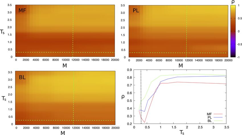
of the number M of sequences in the alignment (cf. also the bottom–right plot in figure
3 in which the other plots are projected at M = M n , that is at the effective number of
sequences of the actual alignment of natural sequences).
All the methods display quite large, temperature–independent correlations (ρ ≥
0.7) at high temperatures and this result gets worse by lowering the temperature. The
temperature that separates the two regimes is of the order of the critical temperature
Tsc1 = 1.5 that separates the two thermodynamic phases discussed in Sect. 3.1.
Unfortunately, the temperature Tsn at which the synthetic sequences are most similar
to the natural ones lies in the frozen phase (Ts ≤ Tsg < Tsc1 ), at which all methods do
not perform well.
Essentially at all temperatures, BL performs better than PL, that performs better
than MF. In particular, at Tsn and M n BL gives ρ = 0.48, PL gives ρ = 0.37 and MF
gives ρ = 0.28. Note that the calculation of the energies by MF and BL take some
minutes on a desktop PC, while by BL it takes ∼ 24 hours.
The number M of sequences needed to reach the best results (cf. figure S7 in the
Supp. Mat.) at high temperatures is ∼ 5000; beyond this number, the value of ρ is
essentially constant. In the low–temperature phase, the performance of the BL is again
constant for M ≥ 5000, while that of the PL is increasing and is comparable to the
BL at M ≈ 20000, compatibly with the fact that PL becomes exact in the limit of
large number of sequences [Arnold and Strauss, 1991]. The MF prediction is slightly
increasing as well, but stays well below that of the other two methods at all values ofProtein Coelvolution 9
M.
Similar comparisons for the other proteins are displayed in figures S8-S10 of the
Supp. Mat. In all cases, the BL algorithm performs better than MF and PL at low
temperatures. PL is always better than MF except for 2ABD at low number M of
sequences (and unfortunately for this protein M n is particularly low). The correlation
coefficient ρ is essentially monotonic with Ts in all cases, and the temperature Tsn
associated with the alignment of natural proteins lies in the bottom part of the plot,
being slightly higher only in the case of 2ABD. At these temperatures the BL algorithm
provides correlation coefficients between 0.4 and 0.6.
To be noted that this performance is achieved with ”typical” sequences. In fact, all
the algorithms we studied return a 4–dimensional tensor Jij (σ, π) of energies indexed
by the pair of sites and the pair of residue in each site. The results discussed above are
obtained comparing the original set of energies J ∗ (σ, π) used to generate the sequences
with the back–calculated tensor projected on a sequence {σi } selected randomly from
the sampling, that is with the matrix Jij (σi , σj ). The results obtained with different
sequences selected from the sampling, and thus comparably likely according to the
underlying Boltzmann distribution, are similar to each other; on the contrary, projecting
the 4–dimensional tensor on a purely random sequence gives a much lower correlation
with the original energies (cf. figure S11 of the Supp. Mat.). The reason for this
behaviour appears to be that a large number of pairs of residue types are never observed
in direct interaction during the sampling.
One can also investigate the dependence of the results on the specific choices done
in the implementation of the algorithms. In the BL it is necessary to choose the number
of steps of the algorithm. According to our tests, the algorithm converges if such a
number of steps is larger than 2000 (cf. figure S12 in the Supp. Mat.). Due to the low
temperature at which we need to sample the space of sequences, one can also investigate
if performing a parallel–tempering sampling [Swendsen and Wang, 1986] instead of a
plain Monte Carlo sampling gives better results in the optimization of the energies. The
results displayed in figure S9 suggest that this is not the case. For the MF algorithm,
one usually employs pseudocounts x to correct the input data [Morcos et al, 2011].
Accordingly with previous results [Lui and Tiana, 2013], the best choice seems to be
x ≈ 1 (cf. figure S13 in the Supp. Mat.).
3.3. Effects of gaps in the sequences
The above analysis was carried out using gap–free sequences, a situation which is quite
idealized. Thus, we calculated the correlation between original and back–calculated
energies in sequences of 1FKJ (made of 107 residues) with 5, 10 and 20 gaps, which
are treated as the 21st type of residue, with null interaction with all the others (cf.
Methods).
The correlation coefficient ρ calculated with MF, PL and BL in presence of gaps is
displayed in figure 4. In the case of MF, the presence of gaps improve the prediction atProtein Coelvolution 10
Figure 3. The Pearson correlation coefficient between energies back–calculated
from the synthetic alignment with the mean–field method (MF), the pseudolikelihood
method (PL) and the Boltzmann learning (BL) algorithm, as a function of the
evolutionary temperature Ts and of the number M of sequences in the synthetic
gap–free alignment for BPI. The dashed lines indicate the temperature Tsn and the
number of sequences M n of the alignment of natural sequences. The bottom–right plot
displays the correlation coefficients for all the protein studied with the three methods
at M = M n .
low temperatures (including Tsn ) and worsen it at large temperatures.
On the other hand, gaps have little effect on the prediction of energies by PL and
BL, slightly worsening the latter because of a more difficult sampling of sequence space.
3.4. Detection of non–interacting residues
The three inversion algorithms can in principle be used to identify the pairs of residues
that do not interact within each protein. This ability is indeed useful because,
since native interactions are optimized by evolution to be as attractive as possible
[Bryngelson and Wolynes, 1987], it is a prerequisite to predict native contacts from the
sequence alignment.
In the model defined by Eq. (2), pairs of residues that are not in contact have
null interaction energy. We tested the ability of the three algorithms to predict that
the energy associated with these pairs is zero. In figure 5 it is shown the distribution
of energies of interacting (∆i,j 6= 0) and non–interacting pairs (∆i,j = 0) for 1BPI,
calculated at various temperatures with the three algorithms (see also figure S14 in
Supp. Mat).
With all algorithms, the distribution of energies of pairs that are not in contact in
the native conformation for a ”typical” sequence (dashed red curve in figure 5), and thus
is expected to be strongly peaked around zero, is actually as broad as the distributionProtein Coelvolution 11
0.8
0.7
0.6 MF
0.5 PL
BL
0.4 BL 5gap
BL 10gap
ρ
0.3 BL 20gap
0.2 MF 5gap
MF 10gap
0.1 MF 20gap
PL 5gap
0 PL 10gap
-0.1 PL 20gap
0 0.5 1 1.5 2 2.5 3 3.5
Ts
Figure 4. The correlation ρ for sequences of 1fkj with gap at M = M n , calculated
with the three algorithms
of interaction energies of native contacts (green dashed curve). Note that if each of the
two curves were normalized independently of the other, the probability that a native
contact displays a negative energy would be much larger than that of a non–native
contact. But the fact that the number of non–native contacts is much larger than that
of native contacts makes it difficult to identify native contacts of a given sequence from
their energy.
On the other hand, the distribution of interaction energies of native contacts
calculated on any sequence (solid green curve in figure 5) reaches values substantially
lower than those of non–native contacts. This result agrees with the idea that a single
sequence displays only few of all possible strongly attractive contacts, and eventually
with the fact that proteins are frustrated systems. Only varying all possible residues in
each site, it is possible to find, beside many unfavourable interactions, also the strongest
attractive ones.
In the case of the MF algorithm, there is no energy below which only native
interactions exist. There is an energy below which native interactions dominate (where
the green and red solid curves cross each other), that contains 0.1% of native interactions,
distributed on 32% of the native contacts, with 0.01% of false negatives, distributed on
28% non–native contacts.
PL gives better results: at low energies (i.e., below the crossing of the green and
red curves in figure 5) there is 0.2% of native interactions, distributed on 42% of native
contacts, with 0.005% of false negatives, distributed on 20% of non–native contacts.
BL is even better, at low energy displaying 1.3% of native interactions, distributed on
98% of native contacts, with 0.02% of false negatives, distributed on 32% of non–native
contacts.Protein Coelvolution 12
The difference between MF, PL and BL is strictly connected to the low value of the
evolutionary temperature Tsn . In fact, true and false positives calculated at higher
temperature (still in the low–temperature phase, but above the freezing transition,
T=102 for 1BPI) give results essentially indistinguishable from BL (cf. figure S15 in
the Supp, Mat.).
Summing up, moving from MF to PL and then to BL, a low–energy tail in the
distribution of all interaction energies of all possible contacts appears that contains
only native interactions. This effect does not occur if one focuses on a single sequence.
The difference in performance of the three algorithms is due to the low evolutionary
temperature of the system.
Finally, the fact that the distribution of energies back–calculated for non–native
pairs is rather symmetrical around zero suggests that the choice of the gauge with
respect to the gap is correct.
3.5. Prediction of native contacts in synthetic alignments by direct coupling
The results described in Sect. 3.4 can be helpful to understand why the analysis
of the direct information (see Sect. 2.4) is so successful [Morcos et al, 2011,
Feinauer et al. 2016, Gueudre et al. 2016], much more than that of contact energies.
Direct information is a way to combine all possible sequence realisations for each pair
of sites, overcoming the overall frustration of the system and the lack of statistics.
Figure 6 shows the number of native and non–native contacts (i.e., true and
false postives, respectively) identified at different thresholds of their normalized direct
information DI/DImax , calculated with MF, PL and PL. The performance of the three
methods seems to be protein–dependent. Looking at the plots, it seems that 1FKJ and
2ABD perform globally better than the other two proteins, displaying a wide range of
normalized DI in which true positives are significantly more than false positives. The
two proteins 1FKJ and 2ABD are those for which the distribution p(q) of Hamming
distances q between the sequences in the alignment are more peaked towards low values
(cf. figure S2 of hte Supp. Mat.), and consequently the system is ”less frozen”. On the
contrary, 1BPI and 1RX4 display a much more structured shape of p(q), typical of the
frozen state of disordered systems, and the contact predictions are worse.
One can be more quantitative and assess the performance of the three algorithms
on the proteins under study by estimators that summarize the results of figure 6. For
example, one can investigate the number of true positives at the value of DI/DImax
at which the number of false positives drops to zero. Calling T P 0% the percentage
of true positives at this value of DI/DImax , one finds that in the case of 1FKJ, MF
gives T P 0% = 3% (it predicts correctly 5 native out of 143), PL gives T P 0% = 20%
(i.e. 30 native contacts) and BL gives T P 0% = 44% (64 contacts). For 1BPI, which
performs globally worst, MF gives T P 0% = 5% T P 0% = 1% and BL T P 0% = 5%.
For the longest proteins (1RX4, made of 159 residues), PL performs best, identifying 52
(T P 0% = 21%) native contacts with no false positives, while BL identifies only 7 trueProtein Coelvolution 13
MF
PL
BL
Figure 5. The distribution of interaction energies calculated by MF, PL and BL for
1BPI at Ts = Tsn for the true native contacts (solid green curve) and for the non–native
contacts (solid red curve). The dashed curves indicate the distribution of native and
non–native energies associated only to a ”typical” sequence (cf. figure S10 of Supp.
Mat.).
positives (T P 0% = 3%).
However, the results depend on the specific estimator used. Using the maximum
MCC (see Methods), BL and MF perform equally well for 1BPI, BL is the best for
1FKJ, MF is the best for 2ABD and PL is the best for 1RX4 (cf. figure S16 in the
Supp. Mat.). The performances of the different algorithms are summarized in figure 7.
From that one learns that the results of the different algorithms depend strongly on the
specific protein and on the estimator used. BL tends to perform better than the other
algorithms, except for 1RX4.
Note that in the above calculations BL seems to have reached convergence, and
extending the optimization does not improve the results (cf. figure S17 in the Supp.
Mat.). Moreover, independent optimizations by BL give identical results (see figure S18Protein Coelvolution 14
1BPI 1FKJ
10000
2ABD 1RX4
number of contacts
1000
100
10
1
0 0.2 0.4 0.6 0.8 1
DI/DImax
Figure 6. The number of native (in green) and non–native (in red) contacts obtained
by MF, PL and MF for the four proteins under study, as a function of the direct
information (DI) normalized to its maximum value (DImax ) obtained for each method.
90
80
MF PL BL
70
60
50
40
30
20
10
0
1BPI TP0% 1FKJ TP0% 2ABD TP0% 1RX4 TP0% 1BPI MCCmax 1FKJ MCCmax 2ABD MCCmax 1RX4 MCCmax
Figure 7. Summary of the percentage of true positives at the value of DI at which
the false positives drop to zero (TP0%) and of maximum MCC
in the Supp. Mat.).
As in the case of energy–based predictions (cf. Sect. 3.4), making use of sequences
generated at an evolutionary temperature larger than Tsn , that is in the low–temperature
but not frozen phase, gives much better prediction results (see figure S19 in the Supp.
Mat.).
According to figure 5, the reason why direct information is more efficient than the
analysis of pair energies seems to be that each homologous sequence displays only a
small fraction of the strongly–interacting native contacts that lie well below the noise
given by non–contacting pairs. Direct information, defined in Eq. (13), sums over all
possible residues in each pair of contacts, and thus captures all possible ways strongly
interacting pairs are placed.Protein Coelvolution 15
10000
true MF
1BPI 1FKJ false MF
true PL
1000 false PL
true BL
false BL
100
10
1
0 0.2 0.4 0.6 0.8 1
10000
2ABD 1RX4
number of contacts
1000
100
10
1
0 0.2 0.4 0.6 0.8 1
DI/DImax
Figure 8. The number of native (in green) and non–native (in red) contacts obtained
by MF, PL and MF for the real alignments of 1BPI, 1FKJ, 2ABD and 1RX4 as a
function of the normalized direct information.
3.6. Native contacts in natural proteins
Finally, we compared the performance of the three algorithms on real sequence
alignments. The performance of all the methods is much worse than that of model
sequences, as shown in figure 8 (cf. also the MCC in figure S20 of the Supp. Mat.).
Also in this case the results are strongly system-dependent. However, BL seems
better than MF and PL since for all proteins there is a range of values of DI for which
the true positives are more than the false positives; correspondingly, the values reached
by MCC associated with predictions of the BL are always larger than those associated
with the other two algorithms (see figure S19).
The results seem quite insensitive with respect to the definition of native contacts,
in that the predictions using different choices of the threshold R on the distance between
residues to define a contact are similar for R > 2.5 Å(cf. figure S21 in the Supp. Mat).
The overall worse performance of the methods to predict native contacts in real
alignments with respect to synthetic ones suggests that the basic assumption which is
common to all of them fails, namely that protein alignments are only approximately
equilibrium realizations of an evolutionary dynamical process.
4. Conclusions
Synthetic protein alignments, generated from a known potential with an equilibrium
sampling of sequence space, are a useful tool to study inversion algorithms to predict
interaction energies and native contacts. The efficiency of such algorithms is strongly
limited by the fact that realistic alignments display features typical of the frozen stateProtein Coelvolution 16
1x10⁶
MF
PL
BL
100000
Time [s]
10000
1000
100
40 60 80 100 120 140 160
Number of residues
Figure 9. The computational time of the three algorithms for proteins of different
lengths on a single core Xeon desktop.
of frustrated systems.
We showed that a Boltzmann Learning algorithm can predict contact energies of
native contacts usually better than mean–field and pseudo–likelihood approximations.
The price for that is a much longer computational time, which is however affordable for
proteins of typical size (cf. figure 9). In principle, pseudo–likelihood calculations can
give comparable results, but need alignments of large numbers of proteins, larger than
those usually available.
The prediction of native contacts from the list of the most attractive two–body
energies gives, in general, limited results, because of the frustration of the system and
because of the strong noise associated with non–interacting pairs (i.e. because of false
positives). While within the subset of native contacts BL can predict native energies
better than the other methods, the energy of non–interacting pairs is very noisy with all
methods, and this fact makes the prediction of native contacts poor with all algorithms.
The calculation of direct information (DI), summed on all possible sequences in each
pair of sites, partially alleviates these problems. However, the three methods perform
differently according to the specific protein. In general, all methods perform better the
less clustered (i.e., less similar to the frozen phases of disordered systems) is the space of
sequences of a protein, as described by the distribution of Hamming distances between
sequence pairs .
The contact prediction in real protein alignments is systematically worse than that
of synthetic proteins with all algorithms, suggesting that the basic assumption at the
basis of all of them, namely that proteins are at equilibrium in sequence space, is
questionable. This fact is not unexpected, due to the low evolutionary temperature
that characterizes realistic alignments and that puts the system in a frozen phase.Protein Coelvolution 17
References
[Göbel et al, 1994] Göbel, U, Sander C, Schneider R, and Valencia A 1994 Correlated mutations and
residue contacts in proteins. Proteins: Struct. Funct. Genet. 18 309
[Anderson, 1978] Anderson, P W 1978 The concept of frustration in spin glasses. J. Less Comm. Met.
62 291
[Cocco et al, 2018] Cocco S, Feinauer C, Figliuzzi M, Monasson R and Weigt M 2018 Inverse statistical
physics of protein sequences: A key issues review. Rep. Prog. Phys. 81 032601
[Morcos et al, 2011] Morcos F, Pagnani A, Lunt B, Bertolino A, Marks D S, Sander C et al. 2011
Direct-coupling analysis of residue coevolution captures native contacts across many protein
families. Proc. Natl. Acad. Sci. USA 108, E1293
[Marks et al, 2011] Marks D S, Colwell L J, Sheridan R, Hopf T A, Pagnani A, Zecchina R and Sander
C 2011 Protein 3D structure computed from evolutionary sequence variation. PloS One, 6,
e28766.
[Procaccini et al, 2011] Procaccini A, Lunt B, Szurmant H, Hwa T and Weigt M 2011 Dissecting the
Specificity of Protein-Protein Interaction in Bacterial Two-Component Signaling: Orphans and
Crosstalks. PloS One 6, e19729.
[Lui and Tiana, 2013] Lui S and Tiana G 2013 The network of stabilizing contacts in proteins studied
by coevolutionary data. J. Chem. Phys. 139 155103
[Jones et al, 2012] Jones D T, Buchan D W A, Cozzetto D and Pontil M 2012 PSICOV: precise
structural contact prediction using sparse inverse covariance estimation on large multiple
sequence alignments. Bioinformatics 28 184
[Eckberg et al, 2013] Ekeberg M, Lävkvist C, Lan Y, Weigt M and Aurell E 2013 Improved contact
prediction in proteins: using pseudolikelihoods to infer Potts models. Phys. Rev. E 87, 620630
[Kamisetty et al, 2013] Kamisetty H, Ovchinnikov S and Baker D 2013 Assessing the utility of
coevolution-based residue-residue contact predictions in a sequence- and structure-rich era. Proc.
Natl. Acad. Sci. USA 110 15674
[Ovchinnikov et al, 2014] Ovchinnikov S, Kamisetty H and Baker D 2014. Robust and accurate
prediction of residue-residue interactions across protein interfaces using evolutionary
information. eLife 3 e02030.
[Ovchinnikov et al, 2017] Ovchinnikov S, Park H, Varghese N, Huang P-S, Pavlopoulos G A, Kim D
E, et al. 2017. Protein structure determination using metagenome sequence data. Science 355
294
[Feinauer et al, 2014] Feinauer C, Skwark M J, Pagnani A and Aurell E 2014 Improving contact
prediction along three dimensions. PLoS Comp. Biol. 10 e1003847
[Dunn et al, 2008] Dunn S D, Wahl L M and Gloor G B 2008. Mutual information without the influence
of phylogeny or entropy dramatically improves residue contact prediction. Bioinformatics 24 333
[Ackely et al, 1985] Ackely D, Hinton G and Sejnowski T 1985. A learning algorithm for boltzmann
machines. Cognitive Science 9 147
[Sutto et al, 2015] Sutto L, Marsili S, Valencia A and Gervasio F L 2015. From residue coevolution
to protein conformational ensembles and functional dynamics. Proc. Natl. Acad. Sci. USA 112,
13567.
[Barrat-Charlaix et al, 2016] Barrat-Charlaix P, Figliuzzi M and Weigt M. 2016 Improving landscape
inference by integrating heterogeneous data in the inverse Ising problem. Scient. Rep. 6, 37812
[Haldane et al, 2016 ] Haldane A, Flynn W F, He P, Vijayan R S K and Levy R M 2016. Structural
propensities of kinase family proteins from a Potts model of residue co-variation. Protein Sci.
25 1378
[Cuturello et al, 2018] Cuturello F, Tiana G, Bussi G 2018 Assessing the accuracy of direct-coupling
analysis for RNA contact prediction. arXiv q-bio 1812.07630
[Darken and Moody, 1991 ] Darken C and Moody J 1991. Towards faster stochastic gradient search.
Proceedings of the Neural Information Processing Systems, Denver, CO, p. 1009Protein Coelvolution 18
[Punta et al, 2012] Punta M, Coggill P C, Eberhardt R Y, Mistry J, Tate, J, Boursnell C, et al. 2012.
The Pfam protein families database. Nucl. Acid. Res. 40, D290
[Rost, 1997] Rost B. 1997. Protein structures sustain evolutionary drift. Folding & Design 2 S19
[Shakhnovich and Gutin, 1993] Shakhnovich E I and Gutin A M 1993. A new approach to the design
of stable proteins. Prot. Engin. 6 793
[Shakhnovich and Gutin, 1993b] Shakhnovich E I and Gutin A M 1993 Engineering of stable and fast-
folding sequences of model proteins. Proc. Natl. Acad. Sci. USA 90 7195
[Fantini et al. 2017] Fantini M, Malinverni D, De Los Rios P and Pastore A 2017. New Techniques for
Ancient Proteins: Direct Coupling Analysis Applied on Proteins Involved in Iron Sulfur Cluster
Biogenesis. Front. Mol. Biosc. 4 40
[Tiana and Sutto, 2011] Tiana G, and Sutto L 2011 Equilibrium properties of realistic random
heteropolymers and their relevance for globular and naturally unfolded proteins. Phys. Rev.
E 84 061910.
[Ramanathan and Shakhnovich, 1994] Ramanathan S and Shakhnovich E I 1994. Statistical mechanics
of proteins with evolutionary selected sequences, Phys. Rev. E 50 1303
[Tiana and Broglia, 2009] Tiana G and Broglia R A 2009 The molecular evolution of HIV-1 protease
simulated at atomic detail. Proteins Struct. Funct. Gen., 76, 895
[Derrida, 1981] Derrida B 1981. Random-energy model: An exactly solvable model of disordered
systems. Phys. Rev. B 24 2613
[Tiana et al. 2000] Tiana G, Broglia R A and Shakhnovich E I 2000 Hiking in the energy landscape in
sequence space: a bumpy road to good folders. Proteins Struct. Funct. Gen. 39 244
[Arnold and Strauss, 1991] Arnold B C and Strauss D 1991 Pseudolikelihood extimation: some
examples. Indian J. Stat. 53 B 233
[Swendsen and Wang, 1986] Swendsen R and Wang J 1986 Replica Monte Carlo simulation of spin
glasses. Phys. Rev. Lett. 57 2607
[Bryngelson and Wolynes, 1987] Bryngelson J D and Wolynes P G 1987 Spin glasses and the statistical
mechanics of protein folding. Proc. Natl. Acad. Sci. USA 84 7524
[Feinauer et al. 2016] Feinauer C, Szurmant H, Weigt M and Pagnani A 2016. Inter-Protein Sequence
Co-Evolution Predicts Known Physical Interactions in Bacterial Ribosomes and the Trp Operon.
PloS One 11 e0149166.
[Gueudre et al. 2016] Gueudrè T, Baldassi C, Zamparo M, Weigt M and Pagnani A(2016. Simultaneous
identification of specifically interacting paralogs and interprotein contacts by direct coupling
analysis. Proc. Natl. Acad. Sci. USA 113 12186You can also read