Crime Scene Shoeprint Retrieval Using Hybrid Features and Neighboring Images - MDPI

Page created by Ryan Mccormick
 
CONTINUE READING
Crime Scene Shoeprint Retrieval Using Hybrid Features and Neighboring Images - MDPI
information
Article
Crime Scene Shoeprint Retrieval Using Hybrid
Features and Neighboring Images
Yanjun Wu 1 , Xinnian Wang 1, *            and Tao Zhang 2
 1   School of Information Science and Technology, Dalian Maritime University, Dalian 116026, China;
     wuyanjun@dlmu.edu.cn
 2   School of Physics and Electronics Technology, Liaoning Normal University, Dalian 116026, China;
     lnnuzt@lnnu.edu.cn
 *   Correspondence: wxn@dlmu.edu.cn
                                                                                                       
 Received: 14 December 2018; Accepted: 21 January 2019; Published: 30 January 2019                     

 Abstract: Given a query shoeprint image, shoeprint retrieval aims to retrieve the most similar
 shoeprints available from a large set of shoeprint images. Most of the existing approaches focus on
 designing single low-level features to highlight the most similar aspects of shoeprints, but their
 retrieval precision may vary dramatically with the quality and the content of the images. Therefore,
 in this paper, we proposed a shoeprint retrieval method to enhance the retrieval precision from
 two perspectives: (i) integrate the strengths of three kinds of low-level features to yield more
 satisfactory retrieval results; and (ii) enhance the traditional distance-based similarity by leveraging
 the information embedded in the neighboring shoeprints. The experiments were conducted on a
 crime scene shoeprint image dataset, that is, the MUES-SR10KS2S dataset. The proposed method
 achieved a competitive performance, and the cumulative match score for the proposed method
 exceeded 92.5% in the top 2% of the dataset, which was composed of 10,096 crime scene shoeprints.

 Keywords: shoeprint retrieval; hybrid features; neighboring images; Fourier-Mellin transform;
 Gabor feature

1. Introduction
      Shoeprint retrieval aims at retrieving the most similar shoeprints that were collected at different
crime scenes, to help investigators to reveal clues about a particular case. In past decades, large
numbers of crime scene shoeprint images were collected and recorded for analysis. When there was
a new case, investigators could manually compare shoeprints derived at the crime scene with those
collected from other crime scenes to reveal clues. It is really difficult and tedious to conduct this
work for a huge number of degraded shoeprints. Therefore, it is necessary to propose a more efficient
automatic shoeprint retrieval method.
      In the past few years, many shoeprint image retrieval methods have been proposed, and they
have demonstrated a good performance in forensic investigations. Most of the existing approaches
focus on designing low-level features to highlight the most similar aspects of shoeprints. From
the perspective of methodology, most of these shoeprint retrieval methods fall into two categories:
(i) retrieval of shoeprints using holistic features [1–13]; and (ii) retrieval of shoeprints using local
features [14–29]. Although both kinds of methods are able to search for shoeprint images with visually
similar shoe patterns, their retrieval precision may vary dramatically among low quality crime scene
shoeprint images. The two main reasons are detailed as follows.
      The first reason may be that the descriptive capability of the low-level feature has its own
deficiencies. Figure 1 shows the illustrative cases of a failure by either approach. Each pair of
shoeprints in Figure 1 does not have the same shoe patterns. The local features (e.g., the Gabor feature)

Information 2019, 10, 45; doi:10.3390/info10020045                         www.mdpi.com/journal/information
Crime Scene Shoeprint Retrieval Using Hybrid Features and Neighboring Images - MDPI
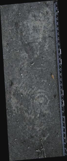
Information 2019, 10, 45                                                                                                                 2 of 15

 Information2018,
Information  2018,9,9,xxFOR
                         FORPEER
                             PEERREVIEW
                                  REVIEW                                                                                               22 of
                                                                                                                                           of 15
                                                                                                                                               15
 cannot distinguish between the visual patterns in Figure 1a, while it accurately handles the visual
 patternsin
patterns
 patterns  inFigure
           in Figure1b.
              Figure    1b.On
                       1b.   Onthe
                            On  theother
                                the  otherhand,
                                     other hand,the
                                           hand,    theholistic
                                                    the holisticfeatures
                                                        holistic features(e.g.,
                                                                 features (e.g.,the
                                                                          (e.g., theFourier-Mellin
                                                                                 the Fourier-Mellinfeature)
                                                                                     Fourier-Mellin    feature)fail
                                                                                                       feature) failto
                                                                                                                fail to
                                                                                                                     to
 make
make    distinctions
       distinctions     in
                       in   Figure
                           Figure   1b,
                                   1b,  while
                                        while  it
                                              it   successfully
                                                  successfully    handles
                                                                 handles   shoeprints
                                                                          shoeprints    in
                                                                                       in   Figure
                                                                                           Figure   1a,
                                                                                                   1a,
 make distinctions in Figure 1b, while it successfully handles shoeprints in Figure 1a, because they     because
                                                                                                        because    they
                                                                                                                  they
 considerthe
consider
 consider   theoverall
           the  overalllayout
                overall   layoutof
                          layout  ofthe
                                  of theimages.
                                     the images.Therefore,
                                         images.    Therefore,  thecomplementary
                                                    Therefore,the
                                                                the complementarydescriptive
                                                                    complementary     descriptivecapability
                                                                                      descriptive   capabilityof
                                                                                                    capability   ofthe
                                                                                                                of  the
                                                                                                                    the
 localand
local
 local andholistic
       and   holisticfeatures
             holistic featuresnaturally
                      features   naturallyinspires
                                 naturally  inspiresus
                                            inspires   usto
                                                       us tointegrate
                                                          to integratetheir
                                                             integrate theirstrengths
                                                                       their  strengthsto
                                                                              strengths  toyield
                                                                                         to  yieldmore
                                                                                             yield moresatisfactory
                                                                                                   more   satisfactory
                                                                                                          satisfactory
 retrieval
retrieval   results.
          results.
 retrieval results.

                                                  (a)
                                                 (a)                                         (b)
                                                                                            (b)
       Figure 1.
      Figure    1. Illustrative
               1.   Illustrative cases
                    Illustrativecases   of
                                        ofaa failure
                                  casesof     failure by   either approach.
                                                       by either
                                                          either   approach. (a)
                                                                  approach.   (a) Holistic
                                                                              (a)Holistic  features may
                                                                                  Holisticfeatures   may yield
                                                                                                           yield more
                                                                                                                  more
       satisfactory    results than local  features.
      satisfactory results than local features. (b)  (b)  Local  features may   yield more   satisfactory results
                                                      (b)Local features may yield more satisfactory results than  than
       holisticfeatures.
      holistic  features.

       The   second
       Thesecond
       The             reason
             secondreason
                       reasonmay may
                                 maybe  bethat
                                        be  thatthe
                                            that    theshoeprints
                                                    the  shoeprintsderived
                                                         shoeprints        derivedfrom
                                                                          derived     fromcrime
                                                                                      from   crimescenes
                                                                                             crime    scenesare
                                                                                                     scenes    areusually
                                                                                                              are   usuallymisaligned,
                                                                                                                    usually    misaligned,
                                                                                                                               misaligned,
 incomplete
 incomplete and
incomplete        anddegraded
                  and    degradedshoeprints
                        degraded        shoeprintsaffected
                                      shoeprints           affectedby
                                                         affected      byby    debris,
                                                                            debris,
                                                                           debris,        shadows
                                                                                       shadows
                                                                                      shadows       andand
                                                                                                   and        other
                                                                                                           other
                                                                                                          other        artifacts.
                                                                                                                   artifacts.
                                                                                                                  artifacts.    Thus,Thus,
                                                                                                                               Thus,     itit isis
 it is difficult
 difficultto
difficult          to
            toretrieveretrieve
                retrievecrime    crime
                           crimescene      scene
                                  sceneshoeprints     shoeprints
                                            shoeprintsusing             using
                                                             usingpair-wise     pair-wise
                                                                       pair-wisesimilarity    similarity
                                                                                     similaritycomputed     computed
                                                                                                   computedfrom  fromjust  from
                                                                                                                         justtwo    just
                                                                                                                              twoimages.  two
                                                                                                                                     images.
 images.
Figure      Figure
 Figure22shows
            showsan   2 shows
                      an  example
                         example anwhere
                                      example
                                      wherethe  thewhere       the similarity
                                                       similarity
                                                      similarity       estimationestimation
                                                                      estimation                   can potentially
                                                                                      canpotentially
                                                                                     can   potentially     benefitfrom
                                                                                                          benefit       benefit
                                                                                                                     from          from the
                                                                                                                            theneighbors.
                                                                                                                           the   neighbors.
 neighbors.
 As   shown      As
                in   shown
                    Figure    in
                             2,  Figure
                                three       2,
                                         samplesthree  A, samples
                                                            B,  and     A,
                                                                        C   B,
                                                                           are and   C   are
                                                                                represented  represented
                                                                                                 as
As shown in Figure 2, three samples A, B, and C are represented as filled circles, and the distance  filled   as  filled
                                                                                                             circles,     circles,
                                                                                                                        and   the    and the
                                                                                                                                    distance
 distance
 betweenAAand
between      between     A  and
                 andBBisisequal   B
                            equalto  is
                                    totheequal     to
                                         thedistance   the
                                              distancebetweendistance
                                                             betweenAAand between
                                                                              andC.    A
                                                                                    C.The and   C.
                                                                                         Thefeature The   feature
                                                                                              featuresimilarity      similarity
                                                                                                         similaritybetween
                                                                                                                       betweenAAandbetween
                                                                                                                                        andBB
 is equal   to  that  betweenthat between
                                  A   and    C,  Athatandis, C,S that
                                                                 (A,  B) is,
                                                                          =  S
                                                                             S ( A,
                                                                               (A,  B
                                                                                   C) ). =
                                                                                         TheS ( A, C )
is equal to that between A and C, that is, S (A, B) = S (A, C) . The neighbors of the three samplesthree
 A  and   B  is  equal   to                                                                            .
                                                                                               neighbors The ofneighbors
                                                                                                                 the  three   of  the
                                                                                                                              samples       are
                                                                                                                                           are
 samples     are
 representedas     represented
                  ascircles.
                      circles.Fromas
                                Fromthecircles.      From
                                         thedistribution
                                              distributionof  the    distribution
                                                                   oftheir
                                                                       theirneighbors of
                                                                               neighborsintheir  neighbors
                                                                                             inFigure           in  Figure
                                                                                                 Figure2,2,ititisismore       2, it
                                                                                                                    morereasonable   is
                                                                                                                            reasonabletomore  to
represented
 reasonable     to  intuitively  let
                           B)
Crime Scene Shoeprint Retrieval Using Hybrid Features and Neighboring Images - MDPI
Information 2019, 10, 45                                                                             3 of 15

      (2) We propose a neighborhood-based similarity estimation (NSE) method, which utilizes the
information contained in neighbors to improve the performance of a shoeprint retrieval method.
The greatest difference, compared to the other existing shoeprint retrieval methods, is that it not
only considers the relationship between every two shoeprints, but also the relationship between
their neighbors;
      (3) We propose a generic manifold based reranking framework, which can narrow the well-known
gap between high-level semantic concepts and low-level features;
      (4) The proposed method can work well for real crime scene shoeprint image retrieval.
The cumulative match score is more than 92.5% in the top 2% of the database, which was composed of
10,096 real crime scene shoeprint images. The evaluation shows our method consistently improves the
retrieval precision and compares favorably with the state-of-the-art.
      The rest of the paper is organized as follows. Section 2 reviews related works on shoeprint
retrieval. Section 3 presents the proposed method. Section 4 provides the experimental results and the
analysis, followed by the conclusions in Section 5.

2. Related Works
      According to the scope of representation, features roughly fall into two categories: holistic features
and local features.
      Methods in the holistic features category usually take the whole image into consideration when
extracting features. Bouridane et al. [1] used a fractal-based feature to retrieve shoeprint images.
They can handle high quality shoeprint images; however, this method is sensitive to variations in
rotations and translations. The moment invariant features were used for shoeprint retrieval [2,3],
and they can work well for complete shoeprints; however, partial shoeprints are not considered.
Chazal et al. [4] and Gueham et al. [5,6] used the Fourier transform to analyze the frequency spectra of
shoeprint images, but the methods are sensitive to partial shoeprints. Cervelli et al. [7–9] utilized the
Fourier transform on the cropped shoeprint images to extract features in frequency domain. However,
these methods are sensitive to geometry transformations. Alizadeh et al. [10] retrieved shoeprints by
using a sparse representation method. They reported good performance, but their method is sensitive
to variations in rotation and translation. Richetelli et al. [11] implemented and tested some shoeprint
retrieval methods on a scene-like shoeprint database, that is, the phase-only correlation (POC) method,
Fourier-Mellin transformation and scale-invariant feature transform (SIFT) method. Results show that
the POC method has better performance than the Fourier-Mellin transformation and the SIFT method;
however, the performances of these methods may drop considerably when applied to degraded crime
scene shoeprints. Kong et al. [12,13] applied a convolutional neural network to extract multi-channel
features, and computed the similarity score using the normalized cross-correlation method. They have
achieved a good performance. However, their algorithm requires a large amount of computation.
      Methods in the local feature category always divide shoeprint into different regions, and
then extract features from these regions. Patil et al. [14] convolved shoeprint images with Gabor
filters, and then divided the filtered images into non-overlapping blocks to extract local features for
shoeprint retrieval. The method shows good performance for partial shoeprints generated from full
shoeprints. Tang et al. [15,16] used an attributed relational graph (ARG) to represent the shoeprint.
In the graph, nodes represent fundamental shapes in shoes, such as lines, circles, ellipses, and so on.
They reported good performance on distortions and partial shoeprints. However, it is a challenge to
handle crime scene shoeprints with random breaks and extrusions, which cannot be represented by
above fundamental geometry shapes. Pavlouet et al. [17,18] applied the maximally stable extremal
regions (MSER) feature to represent shoeprints. However, the performance may drop a lot when
dealing with shoeprint images with noises and distortions. Kortylewsk et al. [19] presented a periodic
pattern-based shoeprint image retrieval method. The method firstly detects periodic patterns of
the shoeprint, and then evaluates the similarity through comparing the Fourier features of the
periodic patterns. The algorithm can deal with shoeprints with periodic patterns. However, it is
Information 2019, 10, 45                                                                                                                           4 of 15

a challenge to handle degraded shoeprint images. Local interest point based methods can work
well for clear shoeprints [20–25], but their performance may vary dramatically among crime scene
shoeprints. The possible reasons may be that the crime scene shoeprints are highly degraded and
randomly occluded, and there are many random extrusions, intrusions or breaks on the shoe patterns.
Nevertheless, the local interest point based methods cannot work well on distinguishing the useful
information from interferences. Kortylewski et al. [26,27] learned a compositional active basis model to
each reference shoeprint, which was used to evaluate against other query images at testing time. The
model can be learned well on high quality reference shoeprints. However, how to represent degraded
crime scene shoeprint images remains a problem. Wang et al. [28] divided a shoeprint into a top region
and a bottom region, and then extracted Wavelet-Fourier-Mellin transform-based features of the two
regions for shoeprint retrieval. The method performs well for its invariant features and matching
score estimation method. Wang et al. [29] proposed a manifold ranking shoeprint retrieval method
that considers not only the holistic and region features but also the relationship between every two
shoeprints. The method achieves a good performance on crime scene shoeprint images, but it neglects
the effect of local features and the contribution of the neighboring shoeprints.

3. Method

3.1. Notations and Formulations
      Let D = {d1 , d2 , · · · , d N } ⊂ Rm     + denote a set of N shoeprint images, and U = q ∪ D =
{u1 ,u2 , . . . ,u N +1 ,u N +1 } ⊂ Rm
                                     + , in which q denotes the query shoeprint. We focus on finding a function
 f : U → R+ that assigns to each shoeprint ui ∈ U a ranking score fi ∈ R+ , 0 ≤ fi ≤ 1 according to
their relevance to the query shoeprint image q. Let f = [f1 , f2 , · · · , fK ], and K = |U| = N + 1.
      Our motivation is to enhance the shoeprint retrieval precision from the following two perspectives:
(i) integrate the strengths of three kinds of low-level features to yield more satisfactory retrieval results;
and (ii) utilize the information contained in the neighboring images to improve the performance of
the shoeprint retrieval method. Therefore, we have two constraints on the ranking score: (i) closer
shoeprint images in multiple feature spaces should share similar ranking scores; and (ii) shoeprint
images with similar neighboring shoeprints should share similar ranking scores.
      We construct the cost function by employing the above two constraints on f. The shoeprint
retrieval problem can be defined as an optimal solution of minimizing the following cost function.
                                                                         2                                           2
                              K   K                                                   K   K                                       K
       f∗ = argminQ(f) = β 1 ∑ ∑ Sij             √1 fi
                                                  Aii
                                                          − √1A f j            + β 2 ∑ ∑ Wij        √1 fi
                                                                                                     Bii
                                                                                                            − √1B f j        + γ ∑ ( fi − yi ) 2      (1)
                  f          i =1 j =1                              jj             i =1 j =1                      jj             i =1

where β 1 , β 2 and γ are the regularization parameters.
    The first term weighted by β 1 is the neighborhood correlation term. Shoeprint images with similar
neighbors should share similar ranking scores. Sij denotes the neighborhood based similarity between
                                                                                  K
ui and u j , and A is a diagonal matrix, in which Aii = ∑ Sij . Intuitively, similarity is usually defined
                                                                                 j =1
as the feature relevance between two images. But it is difficult to use low level features to describe
the shoeprints more clearly, because crime scene shoeprints are usually highly degraded and also
randomly partial. Moreover, the traditional image-to-image similarity measure is sensitive to noises.
One feasible way to deal with this problem is to use the neighborhoods to provide more information.
To this end, we propose a neighborhood-based similarity estimation (NSE) method which regards
the neighbors of the images as their features, the more similar neighbors the images have, the higher
similarity value they should share. Formally, for shoeprint images ui and u j , the neighborhood-based
similarity between the two images can be defined as follows:

                                              ∑               ∑           Wmn
                                                                                          Nk 0 (ui ) ∩ Nk 0 u j
                                                                                                                  
                                         u m ∈ N ( ui ) u n ∈ N ( u j )
                           Sij = aS                                              + aC                                                                 (2)
                                                                                          Nk 0 (ui ) ∪ Nk 0 u j
                                                                                                                 
                                              |N(ui )| N u j
Information 2019, 10, 45                                                                                                                                  5 of 15

where aS and aC are the weighted parameters, and aS + aC = 1. Wmn denotes the hybrid feature
similarity between shoeprint image um and un . N(ui ) = Nk (ui ) ∪ ui , Nk (ui ) denotes the k nearest
neighbors of ui , which is acquired based on the hybrid feature similarity Wij .|•| represents the
cardinality of a set. Nk 0 (ui ) denotes the k nearest neighbors of ui , and they are acquired based
                                            
on the region feature similarity Sr ui , u j that can be calculated according to Equations (7)–(19) in [28].
Here we defined Sij = 1 for ui = u j .
     The second term weighted by β 2 is the smoothness term. The shoeprint images nearby in the
feature space should share similar ranking scores. Wij denotes the hybrid feature similarity between
                                                                                            K
ui and u j , and B is a diagonal matrix, in which Bii = ∑ Wij .
                                                                                           j =1
      The third term weighted by γ is the fitting term. y = [y1 , y2 , . . . , yK ]T is a vector, in which yi = 1,
if ui is the query, and yi = 0 otherwise.
      Equation (1) can also be generalized as a multiple similarity measures manifold ranking frame
work, which can be formulated as follows:
                                                                                                                         2
                                                            P   K     K ( p)                                                        K
             [f∗ , β∗ ] = argminQ(f) =                    ∑ ∑ ∑ β p Wij  q 1( p) fi                   −    r 1 fj            + γ ∑ ( fi − yi ) 2
                                      f,β                                    Cii                               ( p)
                                                         p =1 i =1 j =1                                      C jj                  i =1
                                                                                                                                                             (3)
                                P
             subject to ∑ β p = 1, β p ≥ 0.
                               p =1

where W( p) denotes the adjacency matrix calculated using the pth similarity measure, P denotes the
                                                                                                                   ( p)        K    ( p)
number of similarity measures, and C( p) is a diagonal matrix, and Cii = ∑ Wij . β p represents the
                                                                                                                           j =1
pth regularization parameter. Let β = [ β 1 , β 2 , . . . , β P ].

3.2. Solution
     We solve the optimal question in Equation (3) by constructing a Lagrange function. To get an
                                                         q
optimal regularization parameter β, we replace β p with β p , where q > 1. Therefore, the Lagrange
function is defined as follows:
                                                                                                 2
                                                                                                                                                      !
                           P    K      K                                                                 K                                 P
                                                         1                             1
                       ∑∑∑                                                                               ∑                                 ∑ βp − 1
                                             q   ( p) 
                                                                                                           ( fi − yi ) 2 + α
                                                                                                   
         L(β, α) =                          β p Wij  q                   fi − r               fj  + γ                                                     (4)
                      p =1 i =1 j =1                                ( p)             ( p)
                                                                                                   
                                                                                                            i =1                          p =1
                                                                Cii                 C jj

                ∂L(β,α)                       ∂L(β,α)
      Letting     ∂β p         = 0, and         ∂α          = 0, we can get

                                                                                                           2
                                                    K   K
                                            q −1                               1                   1
                                                   ∑ ∑ Wij
                                                                ( p)                                         
                                       qβ p                          
                                                                      q               fi − r                  −α = 0
                                                                                                           fj                                               (5)
                                                   i =1 j =1                    ( p)                ( p)
                                                                               Cii                 C jj

                                                                           P
                                                                           ∑ βp − 1 = 0                                                                      (6)
                                                                       p =1
Information 2019, 10, 45                                                                                                                              6 of 15

      Then, β p can be acquired as follows:
                                                                              2 1/(q−1)
                                                    K
                                                  ( p)      K
                                         1/ ∑ ∑ Wij  q 1( p) fi − r 1( p) f j  
                                                                                  
                                                   i =1 j =1                    Cii                  C jj
                                 βp =                                                                                                                    (7)
                                                                            2 1/(q−1)
                                                                             
                                        P    K K  ( p)
                                        ∑ 1/ ∑ ∑ Wij  q 1( p) fi − r 1 f j  
                                                                                
                                                                        ( p)          Cii
                                        p =1            i =1 j =1                                           C jj

      Then, we update f by using the new β p . When β p is fixed, we can get
                                                                                                                           2
                                             P      K       K                                                                       K
                                                                                        1                          1
                                          ∑ ∑ ∑ β p Wij                                                                        + γ ∑ ( fi − yi )
                                                                 q       ( p) 
             f∗ = argminQ(f) =                                                                                                                    2
                                                                                                                              
                                                                              
                                                                             q                    fi − r                  fj                           (8)
                           f,β            p =1 i =1 j =1                                    ( p)                    ( p)             i =1
                                                                                        Cii                        C jj

      The matrix-vector formulation of the function is:
                                                            P
                                                             1 q T ( p)   1
                                        Q (f) =         ∑    4
                                                               β p f L f + γ (f − y)T (f − y)
                                                                          2
                                                                                                                                                         (9)
                                                        p =1

                 p           p
where L( p) = I − C( p) W( p) C( p) , which represents a symmetric normalized Laplacian matrix.
    Differentiation Q(f) with respect to f yields
                                                                                      !
                                                            P
                                                            ∑
                                                                 q
                                                                β p L( p )   + γI f − γy = 0                                                           (10)
                                                         p =1

      The ranking score can be obtained as follows:
                                                                                                   ! −1
                                                                     P
                                                                     ∑
                                                        ∗                   q
                                                     f =                   β p L( p )   + γI                γy                                         (11)
                                                                    p =1

      The algorithm is summarized in Algorithm 1.

 Algorithm 1. Solution to the retrieval problem
 Input: The affinity matrix W( p) , the initial ranking score list y. Iteration number T, tuning parameter q.
 Output: The final ranking score list f∗ .
 1: Set r = 0, set β (0) = [1/P, 1/P, . . . , 1/P], assign y to f(0) .
                                                                                p          p
 2: Compute the degree matrix C( p) and the Laplacian matrix L( p) = I − C( p) W( p) C( p)
                                                         ! −1
                                             P      q
 3: Update ranking score f(r) =            ∑ β p L( p) + γI                   γy
                                          p =1
 4: Update β(r) using Equation (7).
 5: Let r = r + 1. If r > T, quit iteration and output final ranking score list f∗ = f(T ) , otherwise go to 3.

3.3. The Affinity Matrix Computation Mothod
     In [28], a Wavelet-Fourier-Mellin transform and Similarity Estimation (WFSE) based method
is proposed to compute the matching score. The WFSE method has been applied successfully in
forensic practice when retrieving crime scene shoeprint images, but it does not take into consideration
the local patterns of the shoeprint. Generally, our observation of objects usually is a continuously
Information 2019, 10, 45                                                                             7 of 15

improving process from the whole to the parts and to the details. Inspired by this rule, we propose a
hybrid holistic, region and local features to compute the matching score, which follows the rules of our
observation to objects. We define the hybrid feature similarity as follows:
                                                                                         
                                W(i, j) = br Sr ui , u j + bh Sh ui , u j + bl Sl ui , u j            (12)

where br , bh and bl denote the weighted parameters, and br + bh + bl = 1.
      For a shoeprint image ui , the extraction process for its hybrid holistic, region and local features
has following six main steps.
      Step 1: Acquire and normalize the shoeprint image.
      Step 1.1: Acquire the binarized shoeprint image. The shoeprint image is firstly split into a grid of
cells, and then a thresholding method (e.g. Otsu’s method) is applied to each cell to extract sub
shoeprints. Finally, morphological operations are utilized to eliminate small holes and smooth edges.
      Step 1.2: Resolution and orientation normalization. The shoeprint images are rescaled to a
predefined resolution measured in dots per inch (DPI). And then we normalize the shoeprint image by
using the Shoeprint Contour Model (SPCM) proposed in [28].
      Step 2: The normalized shoeprint image ui is divided into the top region and the bottom region,
and they are denoted as Stop (i ) and Sbottom (i ), respectively.
      Step 3: The shoeprint image ui and its two regions Stop (i ) and Sbottom (i ) are decomposed at a
specified number of levels by using the Haar Wavelet. We can acquire one approximation and three
details. The coefficients can have the following forms:
                                      n                                     o
                                         (u )
                           FW(ui ) = FW i (l, h, v) 0 ≤ l ≤ L, h, v = 0, 1
                                        n (Stop (i))                                  o
                           FW Stop (i ) = FW          (l, h, v) 0 ≤ l ≤ L, h, v = 0, 1                (13)
                                              n                                          o
                                                (S       (i ))
                           FW(Sbottom (i )) = FW bottom (l, h, v) 0 ≤ l ≤ L, h, v = 0, 1

where L is the maximum level. To avoid merging the useful neighbor patterns, L should be able to
meet the criterion: 2 L−1 ≤ Dmin , where Dmin represents the minimum distance between two neighbor
patterns, which can be specified interactively.
     Step 4: The Fourier-Mellin transform is applied on each wavelet coefficients to extract features.
     Step 4.1: Calculate the Fourier magnitude of the pre-processed image by using the fast Fourier
transform (FFT);
     Step 4.2: Use a band passed filter proposed in [30] to weaken the effect of the noises, such as small
holes, intrusions, extrusions and broken patterns;
     Step 4.3: Perform the log-polar mapping of the filtered Fourier magnitude acquired in Step 4.2;
     Step 4.4: Calculate the Fourier magnitude of the log-polar mapping calculated in Step 4.3 by using
the FFT;
     Step 4.5: The filtered Fourier-Mellin domain coefficients of FW(ui ) are used as holistic features
                           
and those of FW Stop (i ) and FW(Sbottom (i )) are used as region features. Here, we use FMW(ui ),
               
FMW Stop (i ) and FMW(Sbottom (i )) to denote the holistic and region features of the shoeprint ui .
     Step 5: Construct Gabor filters. The Gabor filter in the spatial domain has the following form:
                                        "               !#
                                               2      2
                                            x0     y0                                 π2
                                                                                        
                                1                                       0
                                                                          
                    G( x, y) =       exp −π      +          exp i2π f x     − exp   −                 (14)
                               δx δy        δx 2   δy 2                               2

where x 0 = x sin θ + y cos θ, and x 0 = x cos θ − y sin θ. We set the values of f , δx and
δy as 0.458, 3 and 3, respectively. Here, we construct Gabor filters in eight orientations
(0◦ , 22.5◦ , 45◦ , 67.5◦ , 90◦ , 112.5◦ , 135◦ , 157.5◦ ) according to Equation (14).
       Step 6: Extraction of local features. A shoeprint image is convolved with the Gabor filters in eight
orientations. Then each filtered shoeprint image is divided into non-overlapping blocks, and there
Information 2018, 9, x FOR PEER REVIEW                                                                                              8 of 15

 are 8 blocks
Information 2019,in10,
                    each
                       45 row and 16 blocks in each column. The standard variance                              σ θ ( m, n ) and the 8mean
                                                                                                                                      of 15
 M θ ( m, n ) of the pixel intensities in each block across all filtered images are used as the local features.
The8local
are  blocksfeature of row
             in each  the shoeprint  image
                           and 16 blocks    ui iscolumn.
                                         in each  defined as The  follows:
                                                                    standard variance σθ (m, n) and the mean
                                        GW (u ) = {σ θ ( m, n ) , M θ ( m, n )}
Mθ (m, n) of the pixel intensities in each block across all filtered images are used as the local features.
                                                                                                         (15)
The local feature of the shoeprint image ui isi defined   as follows:
where θ ∈ {θ1 , θ 2 ,..., θ8 } , m = 1, 2,...,8 and n = 1, 2,...,16 .
                                            GW(ui ) = {σθ (m, n), Mθ (m, n)}                       (15)
    For two shoeprint images ui and u j , the holistic feature similarity Sh ( ui , u j ) between them
where θ ∈ {θ1as
is computed      2 , . . . , θ8 }, m = 1, 2, . . . , 8 and n = 1, 2, . . . , 16.
              , θfollows:
                                                                                                               
     For two shoeprint images ui and u j , the holistic feature similarity Sh ui , u j between them is
computed as follows: S h ( u i , u j ) = (
                                              F M W ( u i ) − F M W ( u i ) )( F M W ( u j ) − F M W ( u j ) )
                                                                                                                       (16)
                                              F M W (u i ) − F M W (u i ) F M W (u j ) − F M W (u j )
                                                                                                           
                                           FMW(ui ) − FMW(ui ) FMW(u j ) − FMW(u j )
                                                   )  (i
                                     
     The regional Sfeature             =
                          h ui , u j similarity                                                                        (16)
                                           FMWS(u     r u  , uFMW
                                                        ) i−i j  between
                                                                   (u ) FMW j
                                                                                them(u is
                                                                                        ) −a FMW
                                                                                          j
                                                                                               weighted
                                                                                                    (u ) sum of correlation
coefficients of both FMW ( S ( i ) ) and FMW( S
                                     top                    ( i ) ) . Please refer to Equation (7)–Equation (19)
                                                                 bottom
     The regional feature similarity Sr ui , u j between them is a weighted sum of correlation
in [28] for details
coefficients of both about
                     FMW how
                           Stop (to
                                  i ) set
                                     
                                       andthe weights
                                            FMW        adaptively.
                                                 (Sbottom (i )). Please  The  local
                                                                           refer    feature similarity
                                                                                 to Equations (7)–(19) in
                                                                                                 
                                                                                                          ( u , ufor)
                                                                                                        S [28]                  l   i     j

details
 betweenabout
          two how to is
              images setcomputed
                         the weights adaptively. The local feature similarity Sl ui , u j between two
                                  as follows:
images is computed as follows:
                                                   ( GW (u ) − GW (u ) )( GW (u          ) − GW ( u j )   )
                                     (      ) GW(u ) − GW(u )
                                                           i              i          j
                                   Sl ui , u j =                                                                                        (17)
                                                    GWi ( u i ) − GW (iu i ) GW  u jj)) −
                                                                             GW((u        GW((uuj j))
                                                                                        − GW
                           Sl u i , u j =                                                                                               (17)
                                              GW(ui ) − GW(ui ) GW(u j ) − GW(u j )

4. Experiments
4. Experiments

4.1. Experiment
4.1. Experiment Configuration
                Configuration

4.1.1.
4.1.1. Dataset
       Dataset
     The  experimentswere
      The experiments   wereconducted
                               conducted onon
                                            twotwo   shoeprint
                                                  shoeprint        datasets.
                                                              datasets.  One isOne     is the MUES-SR10KS2S
                                                                                  the MUES-SR10KS2S          dataset
dataset [28],
[28], and     and shoeprints
           shoeprints  in this in this dataset
                               dataset          were collected
                                        were collected    from realfrom    real scenes.
                                                                        crime   crime scenes.      Theisother
                                                                                           The other            is a
                                                                                                           a public
public available
available        dataset,
          dataset, namednamed     the FID-300
                           the FID-300  datasetdataset
                                                 [26]. [26].
     The
      TheMUES-SR10KS2S
          MUES-SR10KS2Sdataset
                             datasetcontains
                                     containsone
                                               oneprobe
                                                    probesetset
                                                              and  one
                                                                 and onegallery  set.set.
                                                                           gallery     The  gallery
                                                                                          The        setset
                                                                                               gallery   consists of
                                                                                                            consists
72 probe   images,  432  synthetic  versions  of  the  probe    images    and   9592
of 72 probe images, 432 synthetic versions of the probe images and 9592 crime scene    crime    scene   shoeprints.
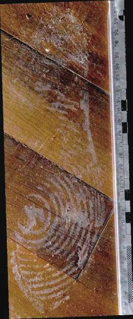
Examples
Examples of crime
              crime scene
                     scene shoeprint
                            shoeprintimages
                                       imagesininthethedataset
                                                        datasetare are  shown
                                                                      shown    in in  Figure
                                                                                   Figure      3. can
                                                                                            3. It  It can   be seen
                                                                                                       be seen  that
that shoeprint
shoeprint      images
           images  withwith
                         samesame  patterns
                               patterns     differ
                                        differ      greatly,
                                               greatly, duedue     to the
                                                               to the      varying
                                                                       varying        imaging
                                                                                 imaging         conditions.
                                                                                            conditions.

                             (a)                                                                    (b)
     Figure 3. Examples
     Figure 3.  Examples of  of crime
                                crime scene
                                       scene shoeprint
                                              shoeprint images
                                                         images inin the
                                                                      theMUES-SR10KS2S
                                                                          MUES-SR10KS2S dataset.dataset. (a)
                                                                                                         (a) The
                                                                                                             The probe
                                                                                                                 probe
     shoeprint
     shoeprint and
                and its
                      its counterparts
                          counterparts from
                                         from real
                                               real crime
                                                    crime scenes
                                                          scenes in
                                                                  in the
                                                                      the gallery
                                                                          gallery set.
                                                                                   set. (b)
                                                                                         (b) Corresponding
                                                                                             Corresponding binarized
                                                                                                              binarized
     versions
     versions of
               of the
                   theprobe
                       probeshoeprint
                              shoeprintandandits
                                               itscounterparts
                                                   counterpartsin
                                                                inthe
                                                                   thegallery
                                                                        galleryset.
                                                                                 set.

       The
       The FID-300
            FID-300 dataset
                      dataset consists
                              consists of of 300
                                             300 probe
                                                  probe shoeprints
                                                         shoeprints and
                                                                     and 1175
                                                                          1175 gallery
                                                                                galleryshoeprints.
                                                                                         shoeprints. The
                                                                                                      The probe
                                                                                                           probe
shoeprint
 shoeprint images were collected from crime scenes by investigators. The gallery shoeprints were
             images  were  collected    from   crime scenes  by  investigators.  The  gallery  shoeprints    were
generated   by using  a gelatine lifter  on the outsole of the reference shoe, and  then by  scanning
 generated by using a gelatine lifter on the outsole of the reference shoe, and then by scanning the   the lifters.
The   gallery
 lifters.     shoeprints
          The gallery     are of very
                      shoeprints        high
                                   are of     quality.
                                           very        Examples
                                                 high quality.    of shoeprints
                                                               Examples          in FID-300
                                                                          of shoeprints       dataset dataset
                                                                                          in FID-300  are shownare
in Figure 4. Figure 4a shows one group of probe shoeprints, and Figure 4b shows their corresponding
shoeprints in the gallery set.
Information 2018, 9, x FOR PEER REVIEW                                                                                       9 of 15

shown in2019,
Information Figure
               10, 45 4.
                   Figure 4a shows one group of probe shoeprints, and Figure 4b shows 9their
                                                                                        of 15
corresponding shoeprints in the gallery set.

                               (a)                                                               (b)
      Figure 4.
      Figure  4. Examples
                 Examples of of the
                                the probe
                                    probe shoeprints
                                          shoeprints and
                                                     and their
                                                          their corresponding
                                                                corresponding reference
                                                                              reference shoeprints
                                                                                        shoeprints in
                                                                                                    in FID-300
                                                                                                       FID-300
      dataset. (a)
      dataset.  (a) The probe shoeprints fromfrom crime
                                                  crime scenes.
                                                         scenes. (b) Corresponding shoeprints of the the probe
                                                                                                         probe
      shoeprints in
      shoeprints  in the
                      the gallery
                          gallery set.
                                  set.

4.1.2.
4.1.2. Evaluation
       Evaluation Metrics
                  Metrics
     The
     The cumulative
           cumulative match
                       match score
                              score used
                                      used in
                                           in [31]
                                               [31] is
                                                    is applied
                                                       applied to  to evaluate
                                                                       evaluate the
                                                                                the performance
                                                                                    performance of
                                                                                                of the
                                                                                                   the method,
                                                                                                       method,
and it is defined as follows:
and it is defined as follows:                                    Rn
                                              CMS(n)= 100                                                 (18)
                                                                 |PR|n
                                                 C M S ( n ) = 100                                         (18)
                                                                    P
where |P| and Rn denote the number of the probe images and the number of gallery images which
match
where the P probe
              and images  in the
                   R denote    thetop n rank,ofrespectively.
                                    number      the probe images and the number of gallery images which
                         n

match
4.2.    the probeEvaluation
     Performance  images in the top n rank, respectively.

4.2. Performance
4.2.1.           Evaluation
       Performance Evaluation of the Proposed Hybrid Features and the Proposed NSE Method

4.2.1.To  test the performance
        Performance      Evaluationofofthe  thehybrid   holistic,
                                                 Proposed     Hybridregion    and local
                                                                         Features          features,
                                                                                     and the    Proposedwe used
                                                                                                             NSE four
                                                                                                                    Methodkinds of
features to retrieve images in the dataset and evaluated the performance of these features according to
their To   test the performance
        cumulative     match score.of We   the also
                                                hybrid   holistic, the
                                                     compared        region   and local features,
                                                                          performance                   we used NSE
                                                                                             of the proposed        four kinds
                                                                                                                           method of
features
with   thattoofretrieve   images
                 the features.      in the
                                  The  firstdataset
                                              kind ofand    evaluated
                                                       feature             the performance
                                                                  is the holistic    feature, and of these   features score
                                                                                                      its matching       according
                                                                                                                                was
to  their  cumulative      match    score.   We   also compared        the  performance       of the
computed according to Equation (16). The second kind of feature is the region feature, in our method, proposed      NSE    method
with
the     that of the features. The
     Wavelet-Fourier-Mellin             first kind
                                    feature          of feature
                                              proposed     in [28]iswas
                                                                      the used
                                                                           holistic   feature,
                                                                                  as the   regionand   its matching
                                                                                                    feature,   and its score    was
                                                                                                                         matching
computed
score         accordingaccording
        was computed        to Equation     (16). The second
                                        to Equation               kind
                                                       (8) in [28].   Theof third
                                                                            feature   is the
                                                                                   kind       region is
                                                                                          of feature   feature,   in our
                                                                                                          the local        method,
                                                                                                                     feature,   and
the   Wavelet-Fourier-Mellin         feature   proposed     in  [28]  was   used  as  the  region   feature,
its matching score was computed according to Equation (17). The fourth kind of feature is the proposed         and   its  matching
score was
hybrid        computed
          features,   and theaccording
                                 matching to Equation
                                              score was(8)     in [28]. The
                                                            computed           third kind
                                                                           according          of feature(12).
                                                                                         to Equation        is the
                                                                                                                 Thelocal  feature,
                                                                                                                       results   are
and   its  matching     score   was   computed      according     to  Equation     (17).  The   fourth
listed in Table 1. For single features, region features have better performance than both holistic and    kind  of  feature   is the
proposed      hybrid    features,   and   the   matching     score   was    computed       according
local features. For the proposed hybrid feature, its cumulative match score is improved 6.6% on          to Equation      (12).  The
results are
average    thanlisted
                  that in  Table
                       of [28]     1. For of
                                 because    single  features, of
                                               the strengths     region
                                                                    threefeatures
                                                                            kinds ofhave      betterfeatures.
                                                                                       low-level      performance        than both
                                                                                                                 The results    also
holistic   and   local features.    For  the  proposed     hybrid    feature,   its cumulative
illustrate that the cumulative match score of the proposed NSE method is improved 10.4% on average   match    score  is  improved
6.6%that
than    on average     than that
            of [28]. Figure         of [28] because
                                5 provides    a visual of   the strengths
                                                         illustration    of theoftop
                                                                                  three    kinds of low-level
                                                                                       10 shoeprint     images infeatures.
                                                                                                                      the rankingThe
results
lists     alsomethod
      of our   illustrateandthat
                               thethe cumulative
                                    compared         matchThe
                                                  method.     score   of theshow
                                                                   results    proposed
                                                                                    that theNSE   methodhybrid
                                                                                               proposed      is improved
                                                                                                                      feature10.4%
                                                                                                                                and
on   average    than  that   of [28]. Figure    5 provides    a  visual
NSE method outperform the work of [28] on the MUES-SR10KS2S database.     illustration    of the  top  10  shoeprint     images    in
the ranking lists of our method and the compared method. The results show that the proposed hybrid
feature Table
           and NSE     method outperform
                  1. Comparison                   the work
                                   of the performance         of [28]
                                                          of our        on the
                                                                  proposed       MUES-SR10KS2S
                                                                              method    with the compareddatabase.
                                                                                                                methods.

          TableApproaches                     The
                1. Comparison of the performance of Cumulative Match
                                                    our proposed      Score
                                                                 method     ofthe
                                                                         with  Topcompared
                                                                                   Percentage
                                                                                           methods.
                                       0.1%     0.2%      0.3%     0.4%       0.5%      1%      2%
                   Approaches
            Holistic feature                 11.9%
                                                      The Cumulative Match
                                                      20.2%    25.2%
                                                                           Score31.9%
                                                                       29.4%
                                                                                 of Top Percentage
                                                                                         39.4%   49.0%
          Region feature [28]                45.2%
                                                 0.1% 64.1%
                                                          0.2% 69.4%
                                                                  0.3%           73.8%
                                                                                   0.4%       75.8%
                                                                                               0.5%      81.8%
                                                                                                          1%         87.5%
                                                                                                                     2%
             Local feature                   11.3%    17.1%    19.0%             20.2%        21.2%      26.8%       32.7%
              Holistic
      The proposed       feature
                    hybrid  feature              11.9%71.4%
                                             53.2%       20.2% 77.6%
                                                                 25.2%            29.4%
                                                                                 81.3%        31.9%
                                                                                              83.1%      39.4%
                                                                                                         87.3%      49.0%
                                                                                                                     89.9%
      The proposed   NSE
             Region featuremethod
                               [28]          53.8%    80.0%    84.1%
                                                 45.2% 64.1% 69.4%               84.7%
                                                                                  73.8%       86.1%
                                                                                              75.8%      89.7%
                                                                                                         81.8%       92.3%
                                                                                                                    87.5%
                   Local feature                  11.3%      17.1%      19.0%      20.2%      21.2%      26.8%      32.7%
        The proposed hybrid feature               53.2%      71.4%      77.6%      81.3%      83.1%      87.3%      89.9%
Information 2018, 9, x FOR PEER REVIEW                                                                                   10 of 15

         The proposed NSE method                53.8%      80.0%      84.1%      84.7%      86.1%      89.7%      92.3%
Information 2019, 10, 45                                                                                                 10 of 15

                                                               (a)

                                                               (b)

                                                               (c)
      Figure 5. Results of our method
      Figure 5.                 method andand the
                                               the compared
                                                    compared methods.
                                                               methods. The top 10 in the ranking list of      of our
                                                                                                                   our
      method
      methodandandthe
                    thecompared
                        compared methods
                                    methodsareare
                                               presented.  Shoeprints
                                                   presented.           encircled
                                                               Shoeprints         by the
                                                                            encircled  bysolid boxesboxes
                                                                                           the solid   are theare
                                                                                                                query
                                                                                                                   the
      shoeprints, and those
      query shoeprints,  andencircled by dotted
                             those encircled  by boxes
                                                  dottedare theirare
                                                         boxes    counterparts.  (a) Wang(a)etWang
                                                                     their counterparts.      al. 2014
                                                                                                     et [28]. (b) [28].
                                                                                                        al. 2014  The
      proposed  hybrid feature.
      (b) The proposed   hybrid (c) The proposed
                                 feature.           neighborhood-based
                                          (c) The proposed                  similaritysimilarity
                                                              neighborhood-based       estimationestimation
                                                                                                    (NSE) method.
                                                                                                               (NSE)
      method.
4.2.2. Comparison with the Traditional Manifold Ranking Method
4.2.2.Zhou
       Comparison        withprovided
               et al. [32]    the Traditional   Manifold
                                         a manifold         Ranking
                                                        based        Method
                                                                 ranking   (MR) algorithm, and the manifold
regularization      term   of our   proposed   ranking    cost
      Zhou et al. [32] provided a manifold based ranking (MR)  function  is basedalgorithm,
                                                                                    on their ideas.
                                                                                               and theTo manifold
                                                                                                         evaluate
the  effectiveness     of our  method,   we  compared      our method   with  the  traditional
regularization term of our proposed ranking cost function is based on their ideas. To evaluate  manifold  ranking
                                                                                                                the
method      [32]. To ensure   a fair comparison,   the  affinity matrixes  used in  both  methods
effectiveness of our method, we compared our method with the traditional manifold ranking method    were the  same
ones
[32]. calculated
       To ensure according       to Equation
                     a fair comparison,    the(2). The cumulative
                                                affinity             match
                                                         matrixes used    inscores  of the algorithms
                                                                             both methods     were theare listed
                                                                                                       same      in
                                                                                                               ones
Table  2. The   results  show   that the performance    of our method  is  approximately   0.7%
calculated according to Equation (2). The cumulative match scores of the algorithms are listed inon average  above
that
Table of 2.
         ZhouTheetresults
                    al. [32].
                           show that the performance of our method is approximately 0.7% on average
above that of Zhou et al. [32].
                           Table 2. Comparison with the traditional manifold ranking method.

                      Table 2. Comparison with the
                                               Thetraditional
                                                    Cumulativemanifold
                                                                Match ranking
                                                                        Score ofmethod.
                                                                                 Top Percentage
               Approaches
                                       0.1%      0.2%      0.3%      0.4%       0.5%      1%                           2%
                   Approaches                         The Cumulative Match Score of Top Percentage
     Manifold ranking method [32]             52.4%    79.6%   83.9%              85.1%       86.3%       89.5%       91.9%
             Our method                           0.1% 81.0%
                                              53.6%       0.2% 84.7%
                                                                 0.3%              0.4%
                                                                                  85.9%       0.5%
                                                                                              86.7%       1%
                                                                                                          89.5%      2%
                                                                                                                      92.5%
       Manifold ranking method [32] 52.4% 79.6% 83.9% 85.1% 86.3% 89.5%                                            91.9%
4.2.3. Comparison
               Ourwith  the Manifold Ranking
                   method             53.6% Based
                                             81.0%Shoeprint
                                                    84.7% Retrieval Method89.5%
                                                            85.9% 86.7%                                            92.5%
      We compared the proposed method with the works of Wang et al. [29] which provided a
4.2.3. Comparison
manifold-based           with the
                      shoeprint   Manifold
                                retrieval         RankingThe
                                             algorithm.            Based Shoeprint
                                                                     method          Retrieval
                                                                              asks forensic      Method
                                                                                              experts   to assign the shoeprint
example
      We an      opinion score
             compared           accordingmethod
                           the proposed        to the similarity
                                                              with thebetween
                                                                          works the   example
                                                                                  of Wang     et and   the query,
                                                                                                  al. [29]   whichinprovided
                                                                                                                      which thea
example     denotes the
manifold-based             shoeprint
                       shoeprint      acquired
                                   retrieval           at the same
                                                  algorithm.           crime
                                                                     The      scene asks
                                                                          method    with the    query experts
                                                                                            forensic    shoeprint.
                                                                                                                 to To  ensure
                                                                                                                     assign     a
                                                                                                                              the
                                                                  T
fair comparison,       the vector
shoeprint example an opinion scorey  =  [ y  , y   , .
                                            1 according
                                                 2     . . , y  ]   used in our  proposed    method     is same  as that
                                                               K to the similarity between the example and the query,    of  [29],
where
in which if ui the
                is the query ordenotes
                     example    the shoeprint        sample that
                                          the shoeprint                has theat
                                                                    acquired   similar  shoe pattern
                                                                                  the same               with the
                                                                                               crime scene        query,
                                                                                                               with        i = 1;
                                                                                                                      the yquery
else      =  0.                                                                           T
     y
shoeprint.
       i          The  cumulative   match      scores        of the  algorithms   are listed  in Table    3.
                To ensure a fair comparison, the vector y = [ y1 , y2 ,..., yK ] used in our proposed method The  experimental
results show that the performance of our method surpasses that of [29]. The cumulative match score of
ours is approximately 3.0% above that of [29] on average.
Information 2019, 10, 45                                                                                          11 of 15

                 Table 3. Comparison with the manifold ranking based shoeprint retrieval method.

                                               The Cumulative Match Score of Top Percentage
               Approaches
                                      0.1%       0.2%      0.3%         0.4%      0.5%        1%         2%
           Wang et al. 2016 [29]     52.6%      76.0%     81.8%         84.5%     85.5%      90.1%     93.5%
              Our method             54.6%      81.7%     86.5%         87.9%     88.9%      90.9%     94.8%

4.2.4. Comparison with the State-of-the-art Algorithms
      We also compared the proposed method with the state-of-the-art shoeprint retrieval methods
on the MUES-SR10KS2S dataset. The results are shown in Table 4. For some state-of-the-art methods
do not release codes, the results listed in Table 4 are achieved by running the codes implemented by
ourselves. In this section, to ensure a fair comparison, the vector y = [y1 , y2 , . . . , yK ]T used in [29] is the
one detailed in Section 3.1. The experimental results show that the cumulative match score of top 2% of
the proposed algorithm is more than 92.5%. It can also be found that the cumulative match score of the
proposed method is improved 5% compared to the work of Wang et al. [28] on top 2% of the ranked
list. The results show that some methods cannot have the similar performance as that reported in the
literatures on the MUES-SR10KS2S dataset. We think the possible reasons may be that: (i) the quality
and quantity of shoeprints in datasets are greatly different; (ii) the codes and experimental settings
may not be the optimal ones.
      Our hardware configuration consists of a 3.33-GHz central processing unit (CPU) with 8-GB
random access memory (RAM). All of the methods are implemented with MATLAB codes. The mean
average running time is applied to evaluate the running times.
                                                           nq
                                                           ∑ T (i )
                                                           i =1
                                                  MAT =                                                              (19)
                                                             nq K

where i denotes the ith query image, T (i ) represents the running time of the ith retrieval, nq denotes
the number of query images, and K is the number of the gallery images.

            Table 4. Comparisons with the state-of-the-art algorithms on the MUES-SR10KS2S dataset.

                                   Performance Reported in the Literature          Performance on Our Dataset
             Methods                                                            The Cumulative       Mean Average
                                                          Gallery Set
                                     Performance                                Match Score of         Running
                                                          Description
                                                                                    Top 2%            Time(ms)
   Kortylewski et al. 2014 [19]       85.7%@20%             #R:1,175                38.64%              0.5696
    Almaadeed et al. 2015 [24]       68.5%@2.5%              #R:400                 34.7%                14.2
       Wang et al. 2014 [28]          87.5%@2%              #S:10,096               87.5%                17.8
       Wang et al. 2016 [29]          93.5%@2%              #S:10,096               91.1%               17.8238
       Kong et al. 2017 [12]          92.5%@20%             #R:1,175                45.6%                186.0
           Our method                     _                 #S:10,096               92.5%                18.2

     To further verify the effectiveness of the proposed method, we compared our proposed method
with the works of Kortylewski et al. [26], Wang et al. [29], Kong et al. [12], Kortylewski [27] and
Kong et al. [13] on a public available database named FID-300 [26]. The results are listed in Table 5.
The results of Kortylewski et al. [26] and Kong et al. [12] are borrowed from Figure 5 in Kong et al. [12].
The results show that our method achieves a good performance on the FID-300 dataset, and the
cumulative match score of our method reaches more than 95.3% in the top 20% of the dataset.
The results also show that there is an improvement of approximately 1.3% compared with the
works of Kong et al. [13] in the top 20% of the ranked list. However, the cumulative match scores of
Information 2019, 10, 45                                                                                      12 of 15

Kong et al. [13] surpass those of ours in the top 1%, 5% and 15% of the ranking list. The main
reason may be as follows. Most of the probe shoeprint images in FID-300 database are of small
size, and some of them only provide a small periodical pattern patch to retrieve shoeprint images.
Kong et al. [13] used a template matching method to search over both translations (with a stride of 2)
and rotations, which can work well for the case that the query image is a small patch. However, our
method does not consider this case.

      Table 5. Comparisons with the state-of-the-art shoeprint retrieval algorithms on the FID-300 dataset.

                                                   The Cumulative Match Score of the Top Percentage
                Method
                                            1%              5%             10%           15%           20%
     Kortylewski et al. 2016 [26]          22.0%           47.5%           58.0%        67.0%         71.0%
       Wang et al. 2016 [29]               67.9%           81.3%           86.3%        91.3%         94.0%
        Kong et al. 2017 [12]              73.0%           82.5%           87.5%        91.0%         92.5%
       Kortylewski 2017 [27]               58.0%           72.0%           79.0%        81.5%         84.0%
        Kong et al. 2018 [13]              79.0%           86.3%           89.0%        91.3%         94.0%
            Our method                     71.8%           81.7%           87.3%        92.0%         95.3%

4.3. Analysis and Discussion
     In this section, we further analyze the effect of different components of the cost function on the
ranking result, which includes the roles of the proposed NSE method and the hybrid feature similarity.
The influence caused by each kind of low-level feature is also discussed.

4.3.1. Effectiveness of the proposed NSE method and the hybrid feature similarity
     In this section, we conducted experiments to verify the effectiveness of the proposed NSE method
and the hybrid feature similarity. We conducted two kinds of experiments by using the MR method
with two different affinity matrixes. The first affinity matrix consists of the hybrid feature similarities
calculated according to Equation (12), and the second affinity matrix is acquired by using the proposed
NSE method. The cumulative match scores of the algorithms are listed in Table 6, and the cumulative
match characteristic curves of the algorithms are shown in Figure 6. The cumulative match scores
show that the performance of our method is approximately 4.1% above that of Zhou et al. [32] with
our proposed hybrid feature similarity on average, and approximately 0.7% on average above that of
Zhou et al. [32] with the affinity matrix computed by using our proposed NSE method. The results
also show that the proposed method using both hybrid feature similarity and NSE method achieves a
higher performance than the one using only the proposed NSE method or the hybrid feature similarity.

                           Table 6. Comparison with the traditional manifold ranking method.

                                                      The Cumulative Match Score of Top Percentage
                       Approaches
                                                   0.1%    0.2%    0.3%      0.4%    0.5%      1%     2%
             Hybrid feature similarity+MR          53.2%   71.8%   78.0%     81.3%   82.7%   87.5%   90.5%
                       NSE+MR                      52.4%   79.6%   83.9%     85.1%   86.3%   89.5%   91.9%
             Our method (Hybrid feature
                                                   53.6%   81.0%   84.7%     85.9%   86.7%   89.5%   92.5%
               similarity +NSE+ MR)
Information 2018, 9, x FOR PEER REVIEW                                                                               13 of 15

                     NSE+MR                        52.4%       79.6%      83.9%     85.1%      86.3%     89.5%      91.9%
        Our method (Hybrid feature                 53.6%       81.0%      84.7%     85.9%      86.7%     89.5%      92.5%
Information 2019, 10, 45                                                                                              13 of 15
            similarity +NSE+ MR)

      Figure 6. Cumulative match characteristic curves of both our method and the traditional manifold
        Figure 6. Cumulative match characteristic curves of both our method and the traditional manifold
      ranking method.
        ranking method.
4.3.2. Effectiveness of Each Kind of Low Level Feature
  4.3.2. Effectiveness of Each Kind of Low Level Feature
      We conducted experiments to verify the effectiveness of each kind of the low level features.
        We conducted
In the experiments,    weexperiments
                            replaced the to    verify the
                                           proposed          effectiveness
                                                        hybrid   feature with of three
                                                                                 each kind
                                                                                       kindsofofthe  low level
                                                                                                 features,         features. In
                                                                                                              and evaluated
  the
the    experiments,
     performance     ofwe  replaced
                        these  featurestheaccording
                                           proposedto    hybrid   feature withmatch
                                                           their cumulative       three kinds
                                                                                        score. of
                                                                                                Thefeatures,
                                                                                                      first kindandofevaluated
                                                                                                                      feature
  the  performance     of these  features   according     to  their cumulative     match  score.
was the hybrid feature of holistic and region feature, and we conducted this kind of experiments  The    first kind  of feature
                                                                                                                            to
  was the
verify  the hybrid   featureofofthe
            effectiveness         holistic
                                      local and    regionThe
                                             features.      feature,
                                                                secondandkind
                                                                            we conducted     this the
                                                                                 of feature was    kindhybrid
                                                                                                           of experiments
                                                                                                                  feature ofto
  verify and
holistic  the effectiveness
              local feature, of andthewe local  features.this
                                           conducted        Thekind
                                                                  second    kind of feature
                                                                       of experiments          was the
                                                                                         to verify   the hybrid      featureofof
                                                                                                            effectiveness
the region features. The third kind of feature was the hybrid feature of region and local feature, of
  holistic and   local feature,  and   we  conducted      this  kind  of experiments    to verify   the  effectiveness    andthe
weregion  features.
    conducted     thisThe
                       kindthird  kind of feature
                              of experiments           was the
                                                  to verify   thehybrid    featureofofthe
                                                                  effectiveness        region  andfeatures.
                                                                                          holistic    local feature,    and we
                                                                                                                 The results
are listed in Table 7. The results show that the method with the proposed hybrid features achieves are
  conducted    this  kind  of  experiments     to  verify  the  effectiveness    of the holistic  features.    The  results  a
  listedperformance
higher   in Table 7. The thanresults
                               the oneshowusingthat
                                                 onlythetwomethod
                                                              of them.with   the proposed
                                                                         Furthermore,        hybrid features
                                                                                         the proposed       hybridachieves
                                                                                                                     features a
  higher
can       performance
     integrate             than of
                the strengths    thethree
                                      one using
                                           kinds only     two of them.
                                                    of low-level           Furthermore,
                                                                    features,              the proposed
                                                                               and each kind    of featureshybrid      features
                                                                                                                can help   the
  can  integrate   the strengths   of  three  kinds   of low-level
proposed method to yield more satisfactory retrieval results.         features,   and each  kind   of  features   can  help  the
  proposed method to yield more satisfactory retrieval results.
                   Table 7. Performance of the proposed method with the three kinds of features.
                    Table 7. Performance of the proposed method with the three kinds of features.
                                                     The Cumulative Match Score of Top Percentage
                      Approaches
                                                     The 0.2%
                                                  0.1%   Cumulative
                                                                 0.3% Match
                                                                          0.4% Score
                                                                                  0.5%of Top1%Percentage
                                                                                                   2%
                     Approaches
       Hybrid feature of holistic and region          0.1%
                                                      48.8%     0.2%
                                                               73.0%       0.3% 80.4%
                                                                         76.6%      0.4%81.3%0.5%86.7% 1%89.3% 2%
       Hybrid feature of holistic and local           33.9%    44.4%     50.2% 54.4% 56.7% 70.4% 77.2%
     Hybrid feature of holistic and region            48.8%     73.0%      76.6% 80.4% 81.3% 86.7% 89.3%
        Hybrid feature of region and local            48.6%    72.2%     75.8% 78.8% 83.9% 88.5% 89.5%
     Hybrid
          Thefeature of holistic
               proposed            and local
                         hybrid feature               33.9%
                                                      53.6%     44.4%
                                                               81.0%       50.2% 85.9%
                                                                         84.7%      54.4%86.7%
                                                                                             56.7%   70.4%
                                                                                                 89.5%   92.5%77.2%
       Hybrid feature of region and local    48.6% 72.2% 75.8% 78.8% 83.9% 88.5% 89.5%
5. Conclusions
         The proposed hybrid feature         53.6% 81.0% 84.7% 85.9% 86.7% 89.5% 92.5%
      In this paper, we proposed an effective shoeprint image retrieval method. In the proposed
  5. Conclusions
method,    we enhance the retrieval precision from two perspectives: (i) integrate the strengths of
three kinds of low-level features to yield more satisfactory retrieval results; and (ii) enhance the
        In this paper, we proposed an effective shoeprint image retrieval method. In the proposed
traditional distance-based similarity by leveraging the information embedded in the neighboring
  method, we enhance the retrieval precision from two perspectives: (i) integrate the strengths of three
shoeprints. The greatest difference between the proposed method and the other existing shoeprint
  kinds of low-level features to yield more satisfactory retrieval results; and (ii) enhance the traditional
retrieval methods is that we not only consider the relationship between every two shoeprints, but also
  distance-based similarity by leveraging the information embedded in the neighboring shoeprints.
the relationships between their neighbors. Our proposed method can also be generalized as a
  The greatest difference between the proposed method and the other existing shoeprint retrieval
generic reranking framework which utilizes information contained in the neighbors to improve
the effectiveness of manifold based method. Experiments on the real crime scene datasets have shown
Information 2019, 10, 45                                                                                     14 of 15

that the performance of the proposed algorithm outperforms not only the traditional manifold ranking
method, but also the state-of-the-art shoeprint retrieval algorithms.

Author Contributions: Y.W. and X.W. conceived the idea and designed the experiments; Y.W. performed the
experiments; Y.W. and T.Z. analyzed the data; Y.W. wrote the original draft; X.W. and T.Z. reviewed and edited the
manuscript; X.W. supervised this work.
Funding: This research received no external funding.
Conflicts of Interest: The authors declare no conflict of interest.

References
1.    Bouridane, A.; Alexander, A.; Nibouche, M.; Crookes, D. Application of fractals to the detection and
      classification of shoeprints. In Proceedings of the International Conference on Image Processing, Vancouver,
      Canada, 10–13 September 2000; pp. 474–477. [CrossRef]
2.    Algarni, G.; Amiane, M. A novel technique for automatic shoeprint image retrieval. Forensic Sci. Int. 2008,
      181, 10–14. [CrossRef] [PubMed]
3.    Wei, C.H.; Hsin, C.; Gwo, C.Y. Alignment of Core Point for Shoeprint Analysis and Retrieval. In Proceedings
      of the International Conference on Information Science, Electronics and Electrical Engineering (ISEEE),
      Sapporo, Japan, 26–28 April 2014; pp. 1069–1072. [CrossRef]
4.    Chazal, P.D.; Flynn, J.; Reilly, R.B. Automated processing of shoeprint images based on the Fourier transform
      for use in forensic science. IEEE Trans. Pattern Anal. Mach. Intell. 2005, 27, 341–350. [CrossRef] [PubMed]
5.    Gueham, M.; Bouridane, A.; Crookes, D. Automatic Classification of Partial Shoeprints Using Advanced
      Correlation Filters for Use in Forensic Science. In Proceedings of the International Conference on Pattern
      Recognition, Tampa, FL, USA, 8–11 December 2008; pp. 1–4. [CrossRef]
6.    Gueham, M.; Bouridane, A.; Crookes, D. Automatic recognition of partial shoeprints based on phase-only
      correlation. In Proceedings of the IEEE International Conference on Image Processing, San Antonio, TX,
      USA, 16 September–19 October 2007; pp. 441–444. [CrossRef]
7.    Cervelli, F.; Dardi, F.; Carrato, S. An automatic footwear retrieval system for shoe marks from real crime
      scenes. In Proceedings of the International Symposium on Image and Signal Processing and Analysis,
      Salzburg, Austria, 16–18 September 2009; pp. 668–672. [CrossRef]
8.    Cervelli, F.; Dardi, F.; Carrato, S. A texture based shoe retrieval system for shoe marks of real crime
      scenes. In Proceedings of the International Conference on Image Analysis and Processing, Catania, Italy,
      8–11 September 2009; pp. 384–393. [CrossRef]
9.    Cervelli, F.; Dardi, F.; Carrato, S. A translational and rotational invariant descriptor for automatic footwear
      retrieval of real cases shoe marks. In Proceedings of the 18th European Signal Processing Conference,
      Aalborg, Denmark, 23–27 August 2010; pp. 1665–1669.
10.   Alizadeh, S.; Kose, C. Automatic retrieval of shoeprint images using blocked sparse representation. Forensic
      Sci. Int. 2017, 277, 103–114. [CrossRef] [PubMed]
11.   Richetelli, N.; Lee, M.C.; Lasky, C.A.; Gump, M.E.; Speir, J.A. Classification of footwear outsole patterns
      using Fourier transform and local interest points. Forensic Sci. Int. 2017, 275, 102–109. [CrossRef] [PubMed]
12.   Kong, B.; Supancic, J.; Ramanan, D.; Fowlkes, C. Cross-Domain Forensic Shoeprint Matching.
      In Proceedings of the 28th British Machine Vision Conference (BMVC), London, UK, 4–7 September 2017.
13.   Kong, B.; Supancic, J.; Ramanan, D.; Fowlkes, C. Cross-Domain Image Matching with Deep Feature Maps.
      arXiv 2018, arXiv:1804.02367,2018.
14.   Patil, P.M.; Kulkarni, J.V. Rotation and intensity invariant shoeprint matching using Gabor transform with
      application to forensic science. Pattern Recognit. 2009, 42, 1308–1317. [CrossRef]
15.   Tang, Y.; Srihari, S.N.; Kasiviswanathan, H. Similarity and Clustering of Footwear Prints. In Proceedings of
      the 2010 IEEE International Conference on Granular Computing, San Jose, USA, 14–16 August 2010;
      pp. 459–464. [CrossRef]
16.   Tang, Y.; Srihari, S.N.; Kasiviswanathan, H.; Corso, J. Footwear print retrieval system for real crime
      scene marks. In Proceedings of the International Conference on Computational Forensics, Tokyo, Japan,
      11–12 November 2010; pp. 88–100. [CrossRef]
Information 2019, 10, 45                                                                                        15 of 15

17.   Pavlou, M.; Allinson, N.M. Automated encoding of footwear patterns for fast indexing. Image Vis. Comput.
      2009, 27, 402–409. [CrossRef]
18.   Pavlou, M.; Allinson, N.M. Automatic extraction and classification of footwear patterns. In Proceedings of
      the 7th International Conference on Intelligent Data Engineering and Automated Learning, Burgos, Spain,
      20–23 September 2006; pp. 721–728. [CrossRef]
19.   Kortylewski, A.; Albrecht, T.; Vetter, T. Unsupervised Footwear Impression Analysis and Retrieval from
      Crime Scene Data. In Proceedings of the Asian Conference on Computer Vision, Singapore, 1–5 November
      2014; pp. 644–658. [CrossRef]
20.   Nibouche, O.; Bouridane, A.; Crookes, D.; Gueham, M.; Laadjel, M. Rotation invariant matching of partial
      shoeprints. In Proceedings of the International Machine Vision and Image Processing Conference, Dublin,
      Ireland, 2–4 September 2009; pp. 94–98. [CrossRef]
21.   Crookes, D.; Bouridane, A.; Su, H.; Gueham, M. Following the Footsteps of Others: Techniques for Automatic
      Shoeprint Classification. In Proceedings of the Second NASA/ESA Conference on Adaptive Hardware and
      Systems, Edinburgh, UK, 5–8 August 2007; pp. 67–74. [CrossRef]
22.   Su, H.; Crookes, D.; Bouridane, A.; Gueham, M. Local image features for shoeprint image retrieval.
      In Proceedings of the British Machine Vision Conference, University of Warwick, Coventry, UK,
      10–13 September 2007; pp. 1–10.
23.   Wang, H.X.; Fan, J.H.; Li, Y. Research of shoeprint image matching based on SIFT algorithm. J. Comput.
      Methods Sci. Eng. 2016, 16, 349–359. [CrossRef]
24.   Almaadeed, S.; Bouridane, A.; Crookes, D.; Nibouche, O. Partial shoeprint retrieval using multiple
      point-of-interest detectors and SIFT descriptors. Integr. Comput. Aided Eng. 2015, 22, 41–58. [CrossRef]
25.   Luostarinen, T.; Lehmussola, A. Measuring the accuracy of automatic shoeprint recognition methods.
      J. Forensic Sci. 2014, 59, 1627–1634. [CrossRef] [PubMed]
26.   Kortylewski, A.; Vetter, T. Probabilistic Compositional Active Basis Models for Robust Pattern Recognition.
      In Proceedings of the 27th British Machine Vision Conference (BMVC), York, UK, 19–22 September 2016.
27.   Kortylewski, A. Model-based IMAGE Analysis for Forensic Shoe Print Recognition. Ph.D. Thesis,
      University of Basel, Basel, Switzerland, 2017.
28.   Wang, X.N.; Sun, H.H.; Yu, Q.; Zhang, C. Automatic Shoeprint Retrieval Algorithm for Real Crime Scenes.
      In Proceedings of the Asian Conference on Computer Vision, Singapore, 1–5 November 2014; pp. 399–413.
      [CrossRef]
29.   Wang, X.N.; Zhan, C.; Wu, Y.J.; Shu, Y.Y. A manifold ranking based method using hybrid features for crime
      scene shoeprint retrieval. Multimed. Tools Appl. 2016, 76, 21629–21649. [CrossRef]
30.   Reddy, B.S.; Chatterji, B.N. An FFT-based technique for translation, rotation, and scale-invariant image
      registration. IEEE Trans. Image Process. 1996, 5, 1266–1271. [CrossRef] [PubMed]
31.   Phillips, P.J.; Grother, P.; Micheals, R. Evaluation Methods in Face Recognition. In Handbook of Face Recognition;
      Jain Anil, K., Li Stan, Z., Eds.; Springer: New York, NY, USA, 2005; pp. 328–348.
32.   Zhou, D.; Weston, J.; Gretton, A.; Bousquet, O.; Scholkopf, B. Ranking on Data Manifolds. In Advances in
      Neural Information Processing Systems 16; Thrun, S., Saul, L.K., Schölkopf, B., Eds.; MIT Press: Cambridge,
      MA, USA, 2003; pp. 169–176.

                           © 2019 by the authors. Licensee MDPI, Basel, Switzerland. This article is an open access
                           article distributed under the terms and conditions of the Creative Commons Attribution
                           (CC BY) license (http://creativecommons.org/licenses/by/4.0/).
You can also read