Cordon- or Link-Based Pricing: Environment-Oriented Toll Design Models Development and Application - MDPI
←
→
Page content transcription
If your browser does not render page correctly, please read the page content below
sustainability

Article
Cordon- or Link-Based Pricing: Environment-Oriented
Toll Design Models Development and Application
Xijie Li 1 , Ying Lv 1, *, Wei Sun 2 and Li Zhou 3
 1    Institute of Transportation System Science and Engineering, School of Traffic and Transportation,
      Beijing Jiaotong University, Beijing 100044, China; 18120844@bjtu.edu.cn
 2    School of Geography and Planning, Sun Yat-Sen University, Guangzhou 510275, China;
      sunwei29@mail.sysu.edu.cn
 3    School of Information, Beijing Wuzi University, Beijing 101149, China; zhoulibit@126.com
 *    Correspondence: ylv@bjtu.edu.cn

 Received: 31 October 2018; Accepted: 25 December 2018; Published: 7 January 2019

 Abstract: This study focuses on an environment-friendly toll design problem, where an acceptable
 road network performance is promised. First, a Traffic Performance Index (TPI)-based evaluation
 method is developed to help identify the optimal congestion level and the management target of a
 transportation system. Second, environment-oriented cordon- and link-based road toll design models
 are respectively proposed through the use of bi-level programming. Both upper-level submodel
 objectives are to minimize gross revenue (the total collected toll minus the emissions treatment
 cost) under different pricing strategies. Both lower-level submodels quantify the user equilibrium
 (UE) condition under elastic demand. Moreover, the TPI-related constraints for the management
 requirements of the network performance are incorporated into the bi-level programming modeling
 framework, which can lead to 0–1 mixed integer bi-level nonlinear programming for toll design
 problems. Accordingly, a genetic algorithm-based heuristic searching method is proposed for the
 two pricing models. The proposed cordon- and link-based pricing models were then applied to a
 real-world road network in Beijing, China. The effects of the toll schemes generated from the two
 models were compared in terms of emissions reduction and congestion mitigation. In this study,
 it was indicated that a higher total collected toll may lead to more emissions and related treatment
 costs. Tradeoffs existed between the toll scheme, emissions reduction, and congestion mitigation.

 Keywords: cordon-based pricing; link-based pricing; toll design; congestion level; emission;
 bi-level programming

1. Introduction
      The continued growth of motor vehicles associated with a large amount of exhaust emissions can
lead to deteriorated ambient air quality, which is not ignored by urban authorities. Road transport,
in particular, contributes significantly to most of the main air pollutants [1]. For example, in Beijing,
China, motor vehicles were over 5.61 million, and the associated annual pollutant discharge was more
than 700,000 tonnes, in 2016. Specifically, it was estimated that the pollutants contributed by motor
vehicles accounted for 86%, 56%, 32%, and 35.5% of carbon monoxide (CO), nitrogen oxides (NOx),
hydrocarbons (HCs), and PM2.5 total emissions, respectively. Therefore, it is necessary to deal with the
pollution problems caused by the urban traffic system.
      Road pricing has been considered to be an effective measure for traffic demand management.
It is essentially based on the principles of economics. Using economic leverage can internalize the
externalities of the traffic system so that traffic flows can be reasonably distributed and the road
resources can be optimized spatiotemporally. The road pricing theory was first proposed by Pigou

Sustainability 2019, 11, 258; doi:10.3390/su11010258                         www.mdpi.com/journal/sustainability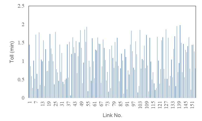
Sustainability 2019, 11, 258                                                                        2 of 16

(1920) and Knight (1924) in the 1920s, and since then many scholars have done a great deal of research
work on the methods and technologies of road pricing [2–8]. For real-world pricing implementations,
Singapore took the lead in implementing the first congestion pricing policy in the world in 1975,
followed by other cities and areas such as London, Hong Kong, Oslo, Gothenburg, and Stockholm [9].
       Generally, toll schemes can be classified in various ways, such as link-based [10],
cordon-based [11], area-based [12], distance-based [13], and time-based schemes [14]. For example,
Yang and Lam [15] proposed a bi-level programming approach for the determination of a coordinated
link toll pattern, in which traffic assignment and road pricing were combined in general road networks.
The link-based pricing aimed to seek the optimal tolls for the network links within a set of system
constraints, and thus, such a toll scheme could be obtained with a certain degree of flexibility while
satisfying various kinds of management requirements. However, link-based pricing is mostly a
theoretical concept that is hard to implement due to the complexity of realistic road networks [16].
Cordon-based pricing allows vehicles to pay tolls to cross a cordon in the inbound direction, in the
outbound direction, or possibly in both directions. Thus, the total number of vehicles that may enter
the encircled area can be restricted. Cordon-based pricing is not necessary to determine toll locations
and levels within the whole road network compared to the link-based one, which seems easier to
implement in real-world management practices. Cordon-based pricing has been discussed, mainly
focusing on optimal toll design [17], public acceptability [18], and policy analysis [19–21]. For example,
Liu et al. [17] tackled the optimal toll design problem using a cordon-based congestion pricing scheme,
where both a time toll and a nonlinear distance toll were levied for each network user’s trip in a pricing
cordon. Nevertheless, when environmental management requirements need to be addressed in the toll
design problem, less attention has been paid to the impact comparison for further understanding the
effectiveness of cordon- and link-based pricing strategies.
       Since a tradeoff exists between system emissions and total travel time [22], more and more
attention has gradually been paid to traffic emission-related pricing studies [23–27]. For example,
Li et al. [23] proposed a two-stage road toll design model for congested road networks with
physical and environmental capacity constraints, which could be used to create a sustainable urban
transportation system. Ma et al. [26] proved that under certain conditions, there exists a free-flow
optimal solution to minimize the generalized system cost, including total travel times and total
emissions. Most previous studies have addressed environmental management targets through the
formulation of minimal emission objectives or capacity constraints, and have used total travel time
(TTT) to measure the congestion of a traffic system. However, TTT is not intuitive enough for real-world
network management, because it may be difficult for local managers and travelers to understand
actual congestion status while minimizing TTT.
       Besides TTT, various indicators are also used for road network performance evaluations. They
are developed based on non-uniform measurement methods by different agencies and are widely
used around the world, such as the Roadway Congestion Index by the Texas Transportation Institute,
calculated based on traffic density, the INRIX Index based on traffic speed, and several comprehensive
indexes used in some Chinese cities (e.g., Beijing, Guangzhou, and Shenzhen) [28–31]. For example,
the Traffic Performance Index (TPI) has been proposed as a comprehensive indicator by the Beijing
Traffic Management Bureau (BTMB). It has obvious advantages in traffic state evaluation from a
network perspective, since it takes road links associated with grades into account [32,33]. However,
these indicators are currently used for traffic performance descriptions, and not enough attention
has been paid to their interconnection with policy making for congestion improvement. Therefore,
it is challenging to integrate a useful indicator into the optimization framework of the pricing model.
The associated toll scheme needs to affect road network performance directly: Meanwhile, the feedback
of the system evaluated by the indicator can result in the adjustment of management strategy.
       The goal of this study was to develop environment-oriented road pricing models. Accordingly,
TPI-based evaluation and optimization methods are proposed to help identify optimal performance
and congestion levels. Then, cordon- and link-based toll design models are respectively developed
Sustainability 2019, 11, x FOR PEER REVIEW 3 of 16
Sustainability
The goal 11,this
2019,of 258 study
was to develop environment-oriented road pricing models. Accordingly, 3 of 16
TPI-based evaluation and optimization methods are proposed to help identify optimal performance
and congestion levels. Then, cordon- and link-based toll design models are respectively developed
through the use of bi-level programming under elastic demand. Meanwhile, TPI-related constraints
through the use of bi-level programming under elastic demand. Meanwhile, TPI-related constraints
are integrated to reflect congestion management requirements of the transportation system. Finally,
are integrated to reflect congestion management requirements of the transportation system. Finally,
the two pricing strategies are discussed based on applications to the road network of Beijing, China.
the two pricing strategies are discussed based on applications to the road network of Beijing, China.
The rest of the study is organized as follows: Section 2 presents evaluation and modeling of traffic
The rest of the study is organized as follows: Section 2 presents evaluation and modeling of traffic
performance and congestion levels. Section 3 formulates environment-oriented cordon- and link-based
performance and congestion levels. Section 3 formulates environment-oriented cordon- and link-
toll design models under elastic demand. Section 4 illustrates a numerical example. Section 5 describes
based toll design models under elastic demand. Section 4 illustrates a numerical example. Section 5
the study case of Beijing, China. Section 6 shows results and discussions, and finally Section 7 concludes
describes the study case of Beijing, China. Section 6 shows results and discussions, and finally Section
this study. In detail, Figure 1 shows the research framework of the study.
7 concludes this study. In detail, Figure 1 shows the research framework of the study.
TPI Definition
TPI Optimization Management target TPI Related
Model for congestion Constraints
TPI-based Bi-level Toll
Design Models
Considering emission
Environment-oriented Environment-oriented
Cordon-based Pricing Model Link-based Pricing Model
Application
Numerical Example Road Network of
Beijing
Analysis of Effects under
Different Pricing Strategies
Figure 1. Research
Figure 1. Research framework of the
framework of the study.
study.
2. Traffic
TrafficPerformance
Performanceand
andCongestion
CongestionLevel
LevelEvaluation
Evaluationand
andModeling
Modeling
In order to assess road network performance, a TPI-based evaluation method is first first introduced,
introduced,
a method
methodfor foridentifying
identifyingoptimal traffic
optimal performance
traffic andand
performance congestion level level
congestion is developed, and TPI-related
is developed, and TPI-
constraints for reflecting performance management requirements in pricing models are
related constraints for reflecting performance management requirements in pricing models are proposed in
this section.
proposed in this section.
2.1.
2.1. Traffic
Traffic Performance
Performance and
and Congestion
Congestion Level
Level Evaluation
Evaluation
According
AccordingtotoReference
Reference[32], thethe
[32], TPI-based
TPI-based evaluation
evaluationmethod can can
method be described in theinfollowing
be described steps.
the following
steps.
2.1.1. Identification of the Congested Road Link
2.1.1. Identification of the Congested Road Link
If the road link is congested, the average speed is less than the threshold of the link with a certain
road If the road
grade, andlink
thusiswe
congested,
have the average speed is less than the threshold of the link with a certain
road grade, and thus we have la,j
v a,j = < ϑj , (1)
t a,jSustainability 2019, 11, 258 4 of 16
where v a,j is the average speed on link a of road grade j, la,j is the length of link a of road grade j,
j = 1, 2, 3, 4 (representing an expressway, arterial road, sub-arterial road, and branch road, respectively),
ta,j is the travel time on link a of road grade j, and ϑ j is the speed threshold of road grade j. For an
expressway, arterial road, sub-arterial road, and branch road, the threshold values are 20, 15, 10, and
10 km/h, respectively.
2.1.2. Calculation of the Network Congested Distance Proportion (CDP)
In order to determine the TPI associated with road network performance and congestion level,
the CDP value should be calculated first. The CDP is a weighted summation of the congested road
links from each road grade in proportion to vehicle kilometers traveled (VKT). Thus, the CDP value
can be obtained based on the following equation:
∑ la,j k a,j ∑ x a,j la,j
4 a∈ A j a= A j
CDP = ∑ 4
, (2)
j =1
∑ la,j · ∑ ∑ x a,j la,j
a∈ A j =1 a ∈ A j
where k a,j equals 1 if v a,j ≤ ϑ j , and 0 otherwise; Aj is the subset of A, representing the set of road grade
j; and xa,j is traffic flow on link a of road grade j.
2.1.3. Determination of the TPI for the Performance and Congestion Level Evaluation
Since the CDP has a corresponding conversion relationship with TPI, the TPI associated with the
performance and congestion level of the road network can be obtained according to Table 1.
Table 1. The conversion relationship between congested distance proportion (CDP) and the Traffic
Performance Index (TPI).
CDP Value/% TPI Performance and Congestion Level
[0,4] [0,2] A (Very smooth)
(5,8] (2,4] B (Smooth)
(8,11] (4,6] C (Lightly smooth)
(11,14] (6,8] D (Moderately congested)
(14,24) (8,10) E (Severely congested)
≥24 10 E (Severely congested)
2.2. Performance and Congestion Level Optimization Model
Assume that the travel time on link a can be presented by the Bureau of Public Roads (BPR)
function of t a ( x a ) = t0a (1 + 0.15( x a /s a )4 ), where t0a and sa represent the free-flow travel time (min) and
the link capacity (vehicle/h), respectively. Based on Equation (1), we have
(
1, v a,j < ϑ j
k a,j = , a ∈ A, ∀ j. (3)
0, v a,j ≥ ϑ j
According to the relationship v a,j = la,j /t a,j , we also have
(
1, x a,j > µ a,j
k a,j = , (4)
0, x a,j ≤ µ a,j
where µ a,j is the flow threshold of congested links, which can be obtained based on the BPR function
1
la,j 4
and presented as µ a,j = s a · ϑ ·t 0 − 1 0.15 .
a,j aSustainability 2019, 11, 258 5 of 16
Let θ donate an arbitrary value between 0 and 1, and then Equation (4) can be expressed
equivalently by the following constraint:
(k a,j − θ )( x a,j − µ a,j ) ≥ 0, k a,j ∈ {0, 1}, a ∈ A. (5)
Thus, the optimal performance and congestion level of a road network can be obtained through
minimizing the CDP value, which can be provided as follows:
∑ la,j k a,j ∑ x a,j la,j
4 a∈ A j a= A j
min ∑ , (6a)
4
j =1
∑ la,j · ∑ ∑ x a,j la,j
a∈ A j j =1 a ∈ A j
subject to
(k a,j − θ )( x a,j − µ a,j ) ≥ 0, k a,j ∈ {0, 1}, a ∈ A, (6b)
∑ frw = dw , w ∈ W, (6c)
r
x a,j = ∑ ∑ f rw δar
w
, a ∈ A, (6d)
w ∈W r ∈ R w
f rw ≥ 0, r ∈ Rw , w ∈ W. (6e)
Apparently, Model (6) can generate the optimal performance and congestion level and help
identify a reasonable management requirement for road network performance.
2.3. Formulation of TPI-Related Constraints
Based on the outputs of Model (6), the management requirement for road network performance
can be identified accordingly. It can be described as the following TPI-related constraints:
∑ la,j k a,j ∑ x a,j la,j
4 a∈ A j a= A j
∑ 4
≤ ρm , (7a)
j =1
∑ la,j · ∑ ∑ x a,j la,j
a∈ A j j =1 a ∈ A j
(k a,j − θ )( x a,j − µ a,j ) ≥ 0, k a,j ∈ {0, 1}, a ∈ A, (7b)
where ρm is the upper bound of the CDP when the network under the performance and congestion
level is m, m ∈ {
h A, B, C,i D, E}. For example, when the management target is set to level m (with
a CDP range of ρ , ρm ), the parameter of ρm in the right-hand side of Equation (7a) thus can be
m
identified according to Table 1. The road network performance should be no worse than level m. Then
Equations (7a) and (7b) can be integrated into the toll design models to reflect the requirement for the
road network performance.
3. Development of the Environment-Oriented Toll Design Models
3.1. Environment-Oriented Cordon-Based Toll Design Model
For a traffic network, the user compares and chooses the shortest path based on the User
Equilibrium (UE) principle, when the generalized link cost is changed by the local manager. Thus,
the decision process between the manager and the user can be described using the following bi-level
programming (BLP) model [34].
The upper-level submodel is
min F (x, y), (8a)
xSustainability 2019, 11, 258 6 of 16
subject to
G(x,y) ≤ 0. (8b)
The lower-level submodel is
min f(x, y), (8c)
y
subject to
g(x,y) ≤ 0, (8d)
where x and y are the decision vectors of the upper- and lower-level submodels, respectively; and
y = y(x) is the reaction or response function, which can be obtained by the lower-level submodel and
used to replace y in the upper-level one.
Accordingly, the BLP method can be applied to the cordon-based toll design problem, wherein the
local manager considers both toll collections and emission externalities in the upper-level submodel
and the UE condition under elastic demand in the lower-level submodel. Thus, a cordon-based bi-level
programming toll design model can be formulated as follows.
The upper-level submodel is
min
τ
∑ τa,j x a,j (τ ) − µ ∑ ea,j ( x a,j (τ )) x a,j (τ ), (9a)
a∈ Ac a∈ Ak
c c
τmin ≤ τa,j ≤ τmax , ∀ a ∈ Ac , (9b)
∑ τa,j x a,j (τ ) − µ ∑ ea,j ( x a,j (τ )) x a,j (τ ) ≥ 0, (9c)
a∈ Ac a∈ Ak
where x a,j (τ ) represents flow on link a of grade j and is the solution to the lower-level problem of UE
under elastic demand.
The lower-level submodel is
Z x a (τ ) Z dw
min Z ( x a , dw ) = ∑ 0
c a (ω, τa )dω − ∑ 0
−1
Dw (ω )dω, (9d)
a∈ Ak w∈Wk
∑ frw = dw , w ∈ W, (9e)
r
x a,j = ∑ ∑ f rw δar
w
, a ∈ A, (9f)
w ∈W r ∈ R w
f rw ≥ 0, r ∈ Rw , w ∈ W, (9g)
where τa,j is a toll on link a; Ac ⊂ A is the subset of links subjected to a cordon toll; Ak ⊂ A is the subset
of links subjected to a link toll; µ is the unit cost of emission; τmax c and τminc are the upper and lower
limits of τa,j for the cordon toll; W is the set of origin-destination (O-D) pairs of the system; Wk is the
subset of O-D pairs within the tolled area, and Wk ⊂ W; dw represents the demand between O-D pair
w, w ∈ W; Rw is the set of paths connecting O-D pair w; δar w equals 1 if route r between O-D pair w uses
link a, a ∈ A, and 0 otherwise; t a,j ( x a,j ) is travel time on link a; and f rw represents traffic flow on path
r. Furthermore, the generalized link travel cost (including both travel time and toll charge, if any) is
given by c a ( x a,j , τa,j ) = t a ( x a,j ) + τa,j .
Through the introduction of the TPI-related constraints proposed in Section 2, an
environment-oriented cordon-based bi-level toll design model can be formulated under elastic demand,
as follows.
In the upper-level submodel, the objective is to minimize gross revenue. The function includes
the total collected tolls and the emissions treatment cost, and can be provided as follows:
min
τ
∑ τa,j x a,j (τ ) − µ ∑ ea,j ( x a,j (τ )) x a,j (τ ), (10a)
a∈ Ac a∈ AkSustainability 2019, 11, 258 7 of 16
where ea,j ( x a,j (τ )) is the carbon monoxide (CO) emission on link a of road grade j (g). In this study, we
considered CO to be a representative indicator of vehicle exhaust emission, and ea,j ( x a,j (τ )) can be
approximatively presented by ea,j x a,j = 4.23605 × 10⁻¹⁵ × la,j × x4a,j + 0.45184 × la,j [35], subject to
the following:
(1) TPI-related constraints,
∑ la,j k a,j ∑ x a,j la,j
4 a∈ A j a= A j
∑ 4
≤ ρm , A j ⊆ Ak , (10b)
j =1
∑ la,j · ∑ ∑ x a,j la,j
a∈ A j j =1 a ∈ A j
(k a,j − θ )( x a,j − µ a,j ) ≥ 0, k a,j ∈ {0, 1}, a ∈ Ak ; (10c)
(2) Toll restrictions,
c c
τmin ≤ τa,j ≤ τmax , ∀ a ∈ Ac , (10d)
where τa,j is a toll on link a of road grade j; and
(3) Gross revenue balance,
∑ τa,j x a,j (τ ) − µ ∑ ea,j ( x a,j (τ )) x a,j (τ ) ≥ 0. (10e)
a∈ Ac a∈ Ak
In the lower-level submodel, this submodel describes the UE problem under elastic demand,
which can be presented as follows,
Z x a (τ ) Z dw
min Z ( x a , dw ) = ∑ 0
c a (ω, τa )dω − ∑ 0
−1
Dw (ω )dω, (10f)
a∈ Ak w∈Wk
subject to the following:
(4) The relationship between path flow and O-D demand,
∑ frw = dw , w ∈ W; (10g)
r
(5) The relationship between flow on link a and path flow (use link a),
x a,j = ∑ ∑ f rw δar
w
, a ∈ A; (10h)
w ∈W r ∈ R w
(6) Non-negative constraint of path flow,
f rw ≥ 0, r ∈ Rw , w ∈ W. (10i)
In the above model, the demand function can be expressed as dw = dw · eκ ·µw , w ∈ Wk , where dw
is the potential demand for the O-D pair, and κ is the parameter reflecting the sensitivity of users to
the generalized travel cost. Consequently, the toll scheme (decision variable of τa,j ) associated with the
traffic flow x a,j can be obtained through solving the above BLP model.
3.2. Environment-Oriented Link-Based Toll Design Model
In comparison, the link-based toll design model has a different toll pattern from the cordon-based
one. It considers links within the tolled area as candidate charging locations. Although the model
expression is similar to the previous cordon-based model, the specific meanings of the modelSustainability 2019, 11, 258 8 of 16
expressions may not be the same. Thus, the environment-oriented link-based toll design model
can be presented as follows.
The objective of the upper-level submodel is also to minimize the gross revenue, wherein the tolls
can be collected from the candidate links within the tolled area:
min
τ
∑ τa,j x a,j (τ ) − µ ∑ ea,j ( x a,j (τ )) x a,j (τ ), (11a)
a∈ Ak a∈ Ak
subject to the following:
∑ la,j k a,j ∑ x a,j la,j
4 a∈ A j a= A j
∑ 4
≤ ρm , A j ⊆ Ak , (11b)
j =1
∑ la,j · ∑ ∑ x a,j la,j
a∈ A j j =1 a ∈ A j
(k a,j − θ )( x a,j − µ a,j ) ≥ 0, k a,j ∈ {0, 1}, a ∈ Ak , (11c)
τmin ≤ τa,j ≤ τmax , ∀ a ∈ Ak , (11d)
∑ τa,j x a,j (τ ) − µ ∑ ea,j ( x a,j (τ )) x a,j (τ ) ≥ 0, (11e)
a∈ Ak a∈ Ak
c
where τmax c
and τmin are the upper and lower limits of τa,j for the link toll.
The lower-level submodel describes the UE problem under elastic demand, which can be
presented as follows:
Z x (τ ) Z dw
a,j
∑ ∑ −1
min Z x a,j , dw = c a,j ω, τa,j dω − Dw (ω )dω. (11f)
a∈ Ak 0 w∈Wk 0
In Equation (11f), the elastic demands refer to all the O-D pairs within the tolled area, which are
different from the cordon-based toll design model (existing in the access links to the cordon). Moreover,
the constraints of the lower-level submodel have similar expressions to those of the cordon-based toll
design model, as shown in Equations (10g)–(10i).
Both the cordon- and link-based toll design methods are based on 0–1 mixed integer bi-level
nonlinear programming models. Accordingly, genetic algorithm-based heuristic solution methods are
proposed for both pricing models.
4. Numerical Example
In this section, we present a hypothetical network for the numerical example to illustrate the
applications of the proposed methods, which are shown in Figure 2. It consists of two O-D pairs,
(1,9) and (2,10). The link travel time could be estimated by using the BPR function. Moreover,
the tolled locations for the cordon-based model are Links 15 and 16, with Ac = {15, 1 6}. The set
of the candidate tolled links for the link-based model is Ak = {1, 2, 3, 4, 5, 6, 7, 8, 9, 10, 11, 12, 13, 14}.
Additionally, the detailed parameters used in the numerical example are presented in Table 2.applications of the proposed methods, which are shown in Figure 2. It consists of two O-D pairs, (1,9)
and (2,10). The link travel time could be estimated by using the BPR function. Moreover, the tolled
locations for the cordon-based model are Links 15 and 16, with Ac ={15,16}. The set of the candidate
tolled links2019,
Sustainability for 11,
the258
link-based model is Ak ={1,2,3,4,5,6,7,8,9,10,11,12,13,14} . Additionally,9 ofthe
16
detailed parameters used in the numerical example are presented in Table 2.
Figure 2. The
The road network of the numerical example.
Table 2. Related parameters of the road network.
Table 2. Related parameters of the road network.
t0a,j
0 (min)
ϑj la ( km) sa ( vehicle/h )
Links Road Grade j Speed Threshold ϑj la (km) sa (vehicle/h)
Links Road Grade j Speed Threshold ta, j (min)
1 2 15.00 0.40 0.40 3000.00
12 2 1 15.00
20.00 0.40
0.35 0.40
0.35 3000.00
2000.00
23 1 1 20.00
20.00 0.35
0.80 0.35
0.80 2000.00
2000.00
34 1 1 20.00
20.00 0.30
0.80 0.30
0.80 2000.00
2000.00
5 1 20.00 0.40 0.40 2500.00
6 1 20.00 0.55 0.55 2000.00
7 1 20.00 0.30 0.30 2000.00
8 2 15.00 0.60 0.60 2000.00
9 1 20.00 0.30 0.30 3000.00
10 1 20.00 0.90 0.90 2000.00
11 2 15.00 1.80 1.80 2500.00
12 2 15.00 0.40 0.40 2000.00
13 2 15.00 0.30 0.30 3500.00
14 2 15.00 0.60 0.60 3000.00
15 / / 4.8 4.8 3000.00
16 / / 5.46 5.46 3000.00
In order to compare the effects of the cordon- and link-based pricing methods, several rules were
regulated as follows:
(1) The area within the cordon (the dotted line) shown in Figure 2 was considered to be a controlled
area by toll schemes, and the regional effects in terms of emissions reduction and congestion
mitigation were investigated and compared under pricing strategies;
(2) Both the cordon- and link-based toll design models had the same O-D pairs and expressions of
elastic demand. Meanwhile, the other parameters of the road network were the same;
(3) In spite of different tolled locations, the total available collected tolls (the sum of the upper limits
of tolls) were the same. For example, the cordon- and link-based tolls had 2 and 14 tolled locations
(or links), and the upper limits of the collected tolls were 7 and 1 for the cordon- and link-based
pricing, respectively. Thus, the total available collected tolls from the road network was 14 for the
two pricing strategies.
Without policy intervention, the CDP could be calculated under the UE condition with a value
of 9.73%. Thus, the congestion level of the road network belonged to level C (lightly smooth).
In order to make a reasonable management target for congestion control under pricing strategies,
the TPI-based evaluation model (Model (6)) needed to first be solved. Therefore, the networkSustainability 2019, 11, 258 10 of 16
performance management target could be predefined based on the optimal congestion level of “very
smooth”, and the right-hand side parameter of Inequality (7a) (the TPI-related constraints) could be
determined with a value of 4% for the two pricing models (Models (10) and (11)).
The results obtained from the two models are presented in Tables 3 and 4. The total travel
demands could be reduced from the original potential demand of 13,500 to 12,686.91 and 12,688.47
under the cordon- and link-based pricing, respectively. Without policy intervention (i.e., under the UE
condition), the total travel time and regional emissions were 51,736.52 min and 64.09 kg, respectively.
Thus, they both decreased under the pricing strategies. Comparatively, the travel time in the control
area was higher under the link-based pricing than under the cordon-based one. In spite of more
regional emissions than under link-based pricing, the pollution treatment cost could be covered by the
higher total toll collected by the cordon-based pricing.
Table 3. Origin-destination (O-D) demands under different policy scenarios.
The Expression of
O-D Pairs Cordon-Based Pricing Link-Based Pricing
Elastic Demand
(1,9) 6500 · e−0.01·u1,9 6342.68 6347.34
(2,10) 7000 · e−0.01·u2,10 6344.23 6341.13
Total travel demand 12,686.91 12,688.47
Table 4. Solutions to the cordon- and link-based pricing models.
Cordon-Based Pricing Link-Based Pricing
Links Road Grade j
Flow Toll Congestion Level Flow Toll Congestion Level
1 2 3563.82 / A 3355.13 0.00 A
2 1 0.00 / B 0.00 0.34 B
3 1 1233.41 / B 753.36 0.00 B
4 1 1956.78 / B 2390.38 0.00 C
5 1 4387.44 / D 3950.75 0.00 D
6 1 1956.78 / B 2390.38 0.00 C
7 1 1775.30 / B 1818.03 0.00 B
8 2 3732.09 / C 4208.41 0.01 D
9 1 3845.55 / C 2886.09 0.13 B
10 1 2330.41 / C 2601.77 0.00 C
11 2 2778.87 / A 2992.20 0.00 A
12 2 2612.14 / A 2132.72 1.00 A
13 2 6175.96 / C 5487.85 0.00 B
14 2 6344.23 / D 6341.13 1.00 D
15 / 6342.68 0.00 / 6347.34 / /
16 / 6344.23 4.37 / 6341.13 / /
Total Travel time (min) 47,617.44 49,248.00
Total emissions (g) 56,690.31 51,639.38
5. Applications to Beijing, China
In this section, both the cordon- and link-based toll design models were applied to the Beijing
2nd Ring Road network (Figure 3). The effects of the two pricing strategies on emission reduction and
congestion mitigation were investigated and are discussed.Total Travel time (min) 47,617.44 49,248.00
Total emissions (g) 56,690.31 51,639.38
5. Applications to Beijing, China
In this section, both the cordon- and link-based toll design models were applied to the Beijing
Sustainability
2nd Ring 11, 258network (Figure 3). The effects of the two pricing strategies on emission reduction
2019, Road 11 of 16
and congestion mitigation were investigated and are discussed.
5 8
1 2 3
2
1 6
10
4 7 12 9 15
4 25 16
11 18 3 21 5 6
13
22 26 30 14 29 17 33 155
34
7 8 9 10 11
19 23 27 31
20 36 24 39 28 43 32 46 35 49
40 44 50
12 13 14 15 16
156 37 41 47
38 52 42 55 45 59 48 63 51 67
56 60 64 68
17 18 19 20 21
157 53 57 61 65
54 72 58 75 62 79 66 83 69 87
73 76 80 84 88 90
22 23 24 25 26 27 28
70 74 77 81 85 89
86 109 91 113
71 92 78 95 82 99
114
110 34 35
96 100 103 106 111
29 93 30 97 31 101 32 104 33 107
112 130 115 133
105 127
94 116 98 119 102 123 134
108 147 40 41
131
120 124 128
36 37 38 39 132 150 135 153
117 121 125
118 136 122 138 126 141 129 144
139 142 145 148 151 154 159
42 43 44 45 46 47 48
158 137 140 143 146 149 152
Figure 3. Beijing 2nd Ring Road network topology.
People living in megacities around the world, such as Beijing, are always eager to travel in
efficient and environmentally friendly ways. However, people in Beijing suffer from air pollution and
traffic congestion, which are partly caused by the urban transportation system. In 2017, the TPI of
the Beijing 2nd Ring Road was 7.0, an increase of 2.6% over last year, during which the congestion
level was “moderately congested” [36]. Therefore, it is urgent to take effective measures to improve
environment and congestion issues. The 2nd Ring Road network is a typical study area of Beijing,
with desired demands for emission control and congestion management. Moreover, the transportation
infrastructures in the area can be well-developed, which is the foundation of implementing the pricing
strategy. Figure 3 shows the topological graph of the study network. The area inside the red dotted
line is the region where the pricing strategy could be applied. In detail, the cordon-based tolls could
be charged at the access links (i.e., Links 155–159), and the link-based tolls could be charged inside
the cordon with the candidate tolled locations of Links 1–154. The blue nodes in the figure represent
the origin and destination points. Similarly, the rules proposed in Section 4 were also employed for
comparison of the effects of both pricing strategies.
6. Results and Discussion
For the study road network, the traffic flow distribution associated with the network CDP value
under the UE condition was also calculated using the system input parameters, which could represent
traffic status without policy intervention. The results showed that under the UE condition, the CDP
value was 6.44%, which corresponded to the road network performance of level B (smooth).
Furthermore, the optimal performance and congestion level of the road network were identified
through the CDP optimization model, and thus, the TPI-related constraints could be formulated to
reflect the road network management target. It was indicated that the optimal CDP value obtained from
Model (6) corresponded to the performance level of A based on Table 1. Accordingly, the right-hand
side parameters of ρ A in constraints (10b) and (11b), respectively, for the cordon- and link-based toll
design models, were 4% for the study network. Then, the toll schemes could be generated from theSustainability 2019, 11, 258 12 of 16
two pricing models. In detail, the tolls charged at the links accessing the cordon for the cordon-based
pricing strategy are provided in Table 5, and the toll scheme for the link-based one is presented in
Figure 4. Correspondingly, the total practical travel demands for the UE, cordon-, and link-based
models were 201,968.9, 163,981, and 199,804, respectively.
Table 5. Toll scheme from cordon-based pricing.
Link 155 156 157 158 159
Toll (min) 61.50 61.60 61.60 40.21 0.00
Total collected toll (min) 807,010.70
Sustainability 2019, 11, x FOR PEER REVIEW 13 of 16
Sustainability 2019, 11, x FOR PEER REVIEW 13 of 16
Figure4.4.Toll
Figure Toll scheme fromlink-based
scheme from link-based pricing.
pricing.
Figure 4. Toll scheme from link-based pricing.
Moreover,
Moreover, thethe
results ofofthe
results theTPI
TPIevaluation, theTTT,
evaluation, the TTT,thetheregional
regional total
total emissions,
emissions, andtotal
and the the total
collected Moreover,
collected
tolls tolls ofthe
of the theresults
study case,ofcase,
study the TPI
could beevaluation,
could theand
TTT,compared
be investigated
investigated the regional
and compared total emissions,
between
between and the
the pricing
the two two total
pricing
strategies,
collected which
strategies, tolls ofare
the study case, could be investigated and compared between the two pricing
summarized
which are summarized in Figure 5. in Figure 5.
strategies, which are summarized in Figure 5.
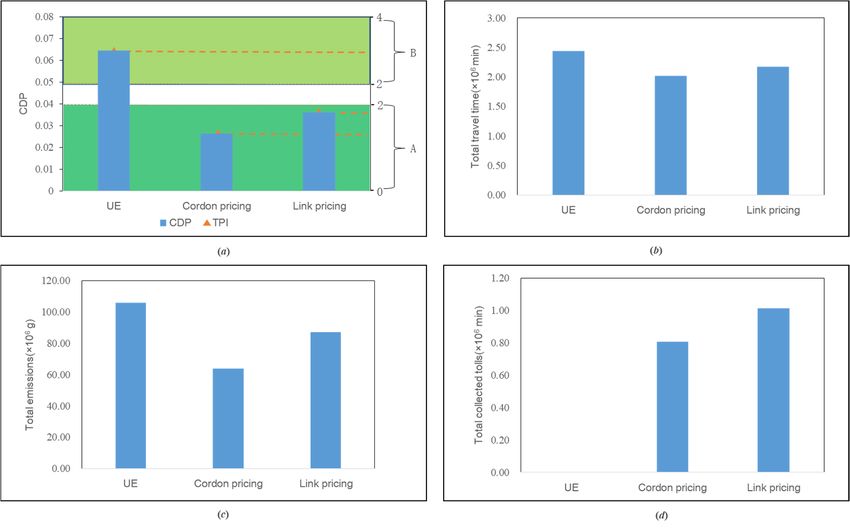
Figure 5. Result comparisons under different policy scenarios: (a) CDP value for TPI-based road
Figure
Figure 5. Result
5. Result
performance comparisons
comparisons
evaluation; under
under
(b) total traveldifferent
different
time (TTT);policy
policy scenarios:
scenarios:
(c) total (a)(a)
emissions; CDP
CDP
and value
(d) value
totalfor TPI-based
for road road
TPI-based
collected tolls.
performance
performance evaluation;
evaluation; (b)(b) total
total traveltime
travel time(TTT);
(TTT); (c)
(c) total
total emissions;
emissions;andand(d)(d)
total collected
total tolls.tolls.
collected
From the perspective of road network performance management, congestion levels are
Frombased
evaluated the onperspective
CDP values of under
road different
network policy performance
scenarios.management,
In detail, the congestion
CDP valueslevels
obtained are
evaluated
from Models based
(10) on
andCDP(11)values underthan
were lower different
thosepolicy
withoutscenarios. In detail, theThey
policy intervention. CDP decreased
values obtained
from
from Models
6.44% under the (10)UEandcondition
(11) weretolower
2.64%than underthose without policy
cordon-based intervention.
pricing and 3.61% They decreased
under from
link-based
6.44% under
pricing. the UE the
Accordingly, condition to 2.64%
congestion levelunder cordon-based
improved from levelpricing
B to A.andThe3.61%
networkunder link-based
performance
pricing.
could Accordingly,
achieve the congestion
a very smooth level improved
status while from levelTTT
pricing. Moreover, B toalso
A. The network
decreased performance
under pricing
strategies, and was reduced from 2.44 × 10 min under the UE condition to 2.02 × 10 min andpricing
could achieve a very smooth status while 6 pricing. Moreover, TTT also decreased 6 under 2.18 ×
strategies, and was reduced from 2.44 × 10⁶ min under the UE condition to 2.02 × 10⁶ min and 2.18 ×Sustainability 2019, 11, 258 13 of 16
From the perspective of road network performance management, congestion levels are evaluated
based on CDP values under different policy scenarios. In detail, the CDP values obtained from Models
(10) and (11) were lower than those without policy intervention. They decreased from 6.44% under the
UE condition to 2.64% under cordon-based pricing and 3.61% under link-based pricing. Accordingly,
the congestion level improved from level B to A. The network performance could achieve a very
smooth status while pricing. Moreover, TTT also decreased under pricing strategies, and was reduced
from 2.44 × 10⁶ min under the UE condition to 2.02 × 10⁶ min and 2.18 × 10⁶ min with the cordon-
and link-based pricing.
Since total practical travel demand could be largely reduced by the cordon-based toll scheme,
the related TTT was much lower than with the link-based one. In order to further understand the
environmental effect of the pricing policies on the study system, the total emissions of the tolled area
were also investigated under different management scenarios. In the study case, the total emissions
were 105.92 × 10³ kg under the UE condition. It was indicated that total emissions could be effectively
reduced by the pricing policies as well. Through implementing the cordon-based pricing strategy,
the related total emissions within the tolled area decreased to 63.85 × 10³ kg, with a reduction of 39.7%.
As for the link-based pricing strategy, the total emissions were reduced by 17.8%, corresponding to
a total of 87.08 × 10³ kg in vehicle exhaust. The pricing policies focusing on emissions controls of
the tolled area may lead to rescheduling routes and potential increases in traffic flows in the links
outside the tolled area. For example, partial vehicles would be forced not to enter the tolled area
under cordon-based pricing. The results showed that the total emissions of the study system did
not increase under the cordon- and link-based polices. The emissions were respectively reduced to
63.94 × 10³ kg and 87.32 × 10³ kg through the cordon- and link-based schemes compared to the UE
condition (106.17 × 10³ kg). Both pricing strategies played positive roles in pollution mitigation.
Comparatively, the cordon-based pricing was better than the link-based one in terms of emissions
reduction in the study network.
In the study, the revenue from the toll collection was mainly used for emissions treatment. Thus,
the pricing strategy with a higher emissions level may increase the total collected toll. For example,
the emissions amount under the link-based pricing was higher than under the cordon one, which
would thus lead to more emissions treatment costs. Accordingly, in order to cover the emissions
treatment costs through pricing, the total collected toll under the link-based pricing needed to be
increased. In detail, the sum of the tolls charged at the links accessing the cordon was 807.01 × 10³
under the cordon-based pricing strategy for the study area. As for the link-based pricing strategy,
a relatively higher total collected toll of 1013.83 × 103 was obtained, comparatively.
Overall, the differences between the cordon- and link-based pricing strategies rely on both the
charging mechanism and the effect in terms of emissions and congestion improvements. From the
aspect of a charging mechanism, the cordon-based pricing only charges travelers who use the links
to access the cordon, and the link-based one considers all the candidate links within the tolled area
and determines the associated toll levels, which may be more complicated to implement in real-world
management practice. Moreover, the cordon toll scheme influences a traveler’s decision, and may
reduce travel demand for entering the tolled area, while the link-based one requires reallocation
of traffic flows under travel demand. Thus, for the numerical example, the cordon toll scheme
could lead to a flow pattern with less TTT, and for the real-world network with less practical travel
demand, the decrease of TTT was more significant compared to the link-based pricing. In terms of the
improvement in emissions abatement, it depends on not only the travel demand, but also the toll design
(the toll locations and levels), which can be investigated in a future study. The factors thus influence the
total collected toll. In the study, the collected toll was mainly used to cover emissions treatment costs.
Under a higher total collected toll level, although it leads to more emissions, the related treatment
costs can be guaranteed. Thus, a tradeoff exists between the toll scheme, emissions reduction, and
congestion mitigation.Sustainability 2019, 11, 258 14 of 16
7. Conclusions
This paper studied environmentally friendly pricing strategies where an acceptable road network
performance is promised. First, a TPI-based evaluation method was proposed in order to help identify
the optimal performance and congestion level of the road network. Then, environment-oriented cordon-
and link-based toll design models were respectively proposed through incorporation of TPI-related
constraints to reflect the performance management target of the traffic system. Both toll design models
were developed based on bi-level programming frameworks. In detail, the upper-level submodel
objectives are to minimize gross revenue, including the total collected tolls and the emissions treatment
costs under different pricing strategies; and the lower-level submodels consider UE conditions under
elastic demand.
A numerical example was used to demonstrate the applications of the developed methods.
Meanwhile, the proposed cordon- and link-based pricing models were applied to a real-world road
network in Beijing, China. The effects of the toll schemes generated from the two models were
compared in terms of emissions reduction and congestion mitigation. In this study, it was indicated
that a higher total collected toll may lead to more emissions and related treatment costs. A tradeoff
existed between the toll scheme, emissions reduction, and congestion mitigation.
Author Contributions: Data curation, software, validation, visualization, and writing—original draft by X.L.;
conceptualization, methodology, supervision, and writing—original draft by Y.L.; formal analysis, supervision,
and writing—review and editing by W.S.; writing—review and editing by L.Z.
Funding: This research was funded by the National Natural Science Foundation of China (71303017),
the Innovative Research Groups of the National Natural Science Foundation of China (71621001), and the Beijing
Intelligent Logistics System Collaborative Innovation Center (BILSCIC-2018KF-03).
Acknowledgments: This research was supported by the National Natural Science Foundation of China (71303017),
the Innovative Research Groups of the National Natural Science Foundation of China (71621001), and the Beijing
Intelligent Logistics System Collaborative Innovation Center (BILSCIC-2018KF-03). The authors thank the
anonymous reviewers for their comments and suggestions that helped in improving the manuscript.
Conflicts of Interest: The authors declare no conflicts of interest.
References
1. European Environment Agency. Emissions of air Pollutants from Transport. Available online:
https://www.eea.europa.eu/data-and-maps/indicators/transport-emissions-of-air-pollutants-8/trans
port-emissions-of-air-pollutants-6 (accessed on 6 December 2018).
2. Verhoef, E.T. The implementation of marginal external cost pricing in road transport. Pap. Reg. Sci. 2000, 79,
307–332. [CrossRef]
3. Bao, Y.; Gao, Z.; Xu, M.; Yang, H. Tradable credit scheme for mobility management considering travelers’
loss aversion. Transp. Res. Part E Logist. Transp. Rev. 2014, 68, 138–154. [CrossRef]
4. He, F.; Yin, Y.; Zhou, J. Deploying public charging stations for electric vehicles on urban road networks.
Transp. Res. Part C Emerg. Technol. 2015, 60, 227–240. [CrossRef]
5. Jiang, Y.B.; Sun, H.J.; Wang, W. Congestion pricing and refund optimization model based on mode choice.
J. Transp. Syst. Eng. Inf. Technol. 2016, 16, 142–147.
6. Gu, Z.; Liu, Z.; Cheng, Q.; Saberi, M. Congestion pricing practices and public acceptance: A review of
evidence. Case Stud. Transp. Policy 2018, 6, 94–101. [CrossRef]
7. Huang, W.J.; Zhang, W.H.; Shen, J.Y.; Jiang, N. Road Congestion Pricing Model Considering Energy
Consumption Measurement. J. Transp. Syst. Eng. Inf. Technol. 2018, 18, 166–172.
8. Wang, Y.; Szeto, W.Y.; Han, K.; Friesz, T.L. Dynamic traffic assignment: A review of the methodological
advances for environmentally sustainable road transportation applications. Transp. Res. Part B Methodol.
2018, 111, 370–394. [CrossRef]
9. Palma, A.D.; Lindsey, R. Traffic congestion pricing methodologies and technologies. Transp. Res. Part C
Emerg. Technol. 2011, 19, 1377–1399. [CrossRef]
10. Wang, G.M.; Gao, Z.Y.; Xu, M. Integrating link-based discrete credit charging scheme into discrete network
design problem. Eur. J. Oper. Res. 2019, 272, 176–187. [CrossRef]Sustainability 2019, 11, 258 15 of 16
11. Liu, Z.; Meng, Q.; Wang, S. Variational inequality model for cordon-based congestion charging under side
constrained stochastic user equilibrium conditions. Transp. A Transp. Sci. 2014, 10, 693–704.
12. Gu, Z.Y.; Shafiei, S.; Liu, Z.Y.; Saberi, M. Optimal distance- and time-dependent area-based pricing with the
Network Fundamental Diagram. Transp. Res. Part C Emerg. Technol. 2018, 95, 1–28. [CrossRef]
13. Daganzo, C.F.; Lehe, L.J. Distance-dependent congestion pricing for downtown zones. Transp. Res.
Part B Methodol. 2015, 75, 89–99. [CrossRef]
14. Zheng, N.; Rérat, G.; Geroliminis, N. Time-dependent area-based pricing for multimodal systems with
heterogeneous users in an agent-based environment. Transp. Res. Part C Emerg. Technol. 2016, 62, 133–148.
[CrossRef]
15. Yang, H.; Lam, W. Optimal road tolls under conditions of queueing and congestion. Transp. Res. Part A
Policy Pract. 1996, 30, 319–332.
16. Kolak, O.İ.; Feyzioğlu, O.; Noyan, N. Bi-level multi-objective traffic network optimization with sustainability
perspective. Expert Syst. Appl. 2018, 104, 294–306. [CrossRef]
17. Liu, Z.; Wang, S.; Meng, Q. Optimal joint distance and time toll for cordon-based congestion pricing.
Transp. Res. Part B Methodol. 2014, 69, 81–97. [CrossRef]
18. Grisolía, J.M.; López, F.; Ortúzar, J.D. Increasing the acceptability of a congestion charging scheme.
Transp. Policy 2015, 39, 37–47.
19. Anas, A.; Hiramatsu, T. The economics of cordon tolling: General equilibrium and welfare analysis.
Econ. Transp. 2013, 2, 18–37. [CrossRef]
20. Aziz, H.M.A.; Ukkusuri, S.V. Exploring the trade-off between greenhouse gas emissions and travel time
in daily travel decisions: Route and departure time choices. Transp. Res. Part D Transp. Environ. 2014, 32,
334–353. [CrossRef]
21. Li, Z.C.; Guo, Q.W. Optimal time for implementing cordon toll pricing scheme in a monocentric city.
Pap. Reg. Sci. 2017, 96, 163–190. [CrossRef]
22. Azari, K.A.; Arintono, S.; Hamid, H.; Davoodi, S.R. Evaluation of demand for different trip purposes under
various congestion pricing scenarios. J. Transp. Geogr. 2013, 29, 43–51. [CrossRef]
23. Li, Z.; Lam, W.; Wang, S.; Sumalee, A. Environmentally Sustainable Toll Design for Congested Road Networks
with Uncertain Demand. Int. J. Sustain. Transp. 2012, 6, 127–155. [CrossRef]
24. Szeto, W.Y.; Wang, Y.; Wong, S.C. The chemical reaction optimization approach to solving the environmentally
sustainable network design problem. Comput. Aided Civ. Infrastruct. Eng. 2014, 29, 140–158. [CrossRef]
25. Ding, D.; Shuai, B.; Zhi, J.C. Impact of Emission Charging to Carpooling in Urban Roads. J. Transp. Syst. Eng.
Inf. Technol. 2015, 15, 26–32.
26. Ma, R.; Ban, X.; Szeto, W. Emission modeling and pricing on single-destination dynamic traffic networks.
Transp. Res. Part B Methodol. 2017, 100, 255–283. [CrossRef]
27. Long, J.; Chen, J.; Szeto, W.; Shi, Q. Link-based system optimum dynamic traffic assignment problems with
environmental objectives. Transp. Res. Part D Transp. Environ. 2018, 60, 56–75. [CrossRef]
28. Schrank, D.; Lomax, T. The 2005 Urban Mobility Report; Texas Transportation Institute: College Station, TX,
USA, 2005.
29. Das, D.K.; Keetse, M.S.M. Assessment of traffic congestion in the central areas of Kimberley city.
Interim Interdiscip. J. 2015, 14, 70–82.
30. Bian, C.; Yuan, C.; Kuang, W.; Wu, D. Evaluation, Classification, and Influential Factors Analysis of Traffic
Congestion in Chinese Cities Using the Online Map Data. Math. Probl. Eng. 2016, 2016, 1693729. [CrossRef]
31. He, F.F.; Yan, X.D.; Liu, Y.; Ma, L. A Traffic Congestion Assessment Method for Urban Road Networks Based
on Speed Performance Index. Procedia Eng. 2016, 137, 425–433. [CrossRef]
32. BTMB. Urban Road Traffic Performance Index; Beijing Municipal Commission of Transport: Beijing, China,
2011. (In Chinese)
33. Lv, Y.; Wang, S.S.; Gao, Z.Y.; Li, X.J.; Sun, W. Design of a heuristic environment-friendly road pricing scheme
for traffic emission control under uncertainty. J. Environ. Manag. 2018. [CrossRef]
34. Sun, H.; Gao, Z.; Wu, J. A bi-level programming model and solution algorithm for the location of logistics
distribution centers. Appl. Math. Model. 2008, 32, 610–616. [CrossRef]Sustainability 2019, 11, 258 16 of 16
35. Yin, Y.; Lawphongpanich, S. Internalizing emission externality on road networks. Transp. Res. Part D
Transp. Environ. 2006, 11, 292–301. [CrossRef]
36. Beijing Transport Institute. Beijing Transport Development Annual Report. Available online: http://www.bj
trc.org.cn/JGJS.aspx?id=5.2&Menu=GZCG (accessed on 6 December 2018). (In Chinese)
© 2019 by the authors. Licensee MDPI, Basel, Switzerland. This article is an open access
article distributed under the terms and conditions of the Creative Commons Attribution
(CC BY) license (http://creativecommons.org/licenses/by/4.0/).You can also read