Compatibility of drought magnitude based method with SPA for assessing reservoir volumes: analysis using Canadian river flows
←
→
Page content transcription
If your browser does not render page correctly, please read the page content below
Preprints (www.preprints.org) | NOT PEER-REVIEWED | Posted: 13 July 2021                       doi:10.20944/preprints202107.0301.v1

             Compatibility of drought magnitude based method with SPA for
             assessing reservoir volumes: analysis using Canadian river flows
             Tribeni C. Sharma1 and Umed S. Panu2*

                                           1 Department of Civil Engineering, Lakehead University, Thunder Bay, ON, P7B 5E1, Canada
                                             (tcsharma @ lakeheadu.ca)
                                           2 Department of Civil Engineering, Lakehead University, Thunder Bay, ON, P7B 5E1, Canada

                                           (uspanu@lakeheadu.ca
                                            * Correspondence: author)

                                           Abstract: The traditional sequent peak algorithm (SPA) was used to assess the reservoir
                                           volume (VR) for comparison with deficit volume, DT, (subscript T representing the
                                           return period) obtained from the drought magnitude (DM) based method with draft
                                           level set at the mean annual flow on 15 rivers across Canada. At an annual scale, the
                                           SPA based estimates were found to be larger with an average of nearly 70% compared
                                           to DM based estimates. To ramp up DM based estimates to be in parity with SPA based
                                           values, the analysis was carried out through the counting and the analytical procedures
                                           involving only the annual SHI (standardized hydrological index, i.e. standardized
                                           values of annual flows) sequences. It was found that MA2 or MA3 (moving average of
                                           2 or 3 consecutive values) of SHI sequences were required to match the counted values
                                           of DT to VR. Further, the inclusion of mean, as well as the variance of the drought
                                           intensity in the analytical procedure, with aforesaid smoothing led DT comparable to
                                           VR. The distinctive point in the DM based method is that no assumption is necessary
                                           such as the reservoir being full at the beginning of the analysis - as is the case with SPA.

                                           Keywords: Deficit volume; drought intensity; drought magnitude; extreme number
                                           theorem; Markov chain; moving average smoothing; standardized hydrological index;
                                           sequent peak algorithm; reservoir volume.

                                           1. Introduction

                                                   A considerable amount of research can be traced to the hydrologic
                                           drought models that focus on the estimation of drought duration and
                                           magnitude (previously termed as severity) using the river flow data. Two
                                           major elements of the hydrologic drought studies have been the truncation
                                           level approach and the analysis by simulation and/or analytical methods. The
                                           analytical methods are pursued by the use of the frequency analyses of
                                           drought events in terms of duration and deficit volumes. The noteworthy
                                           contributions in this area of frequency analyses are that of [1], [2], [3], [4],
                                           among others. The other route in the domain of analytical methods is the use
                                           of the theory of runs, which is well documented in [5 - 13]. Several hydrologic
                                           drought indices have been suggested such as standardized runoff index (SSI)
                                           [14], streamflow drought index (SDI) [15], and standardized hydrologic index
                                           (SHI) [12, 13]. These indices are essentially standardized (statistically) values

                                                                                                                                      1

            © 2021 by the author(s). Distributed under a Creative Commons CC BY license.
Preprints (www.preprints.org) | NOT PEER-REVIEWED | Posted: 13 July 2021 doi:10.20944/preprints202107.0301.v1
of historical stream flows or in some transformed version (normalization in a
probabilistic sense) at the desired time scale. The standardized hydrological
index (SHI) is the standardized value (statistical) of river flows with the mean
0 and the standard deviation equal to 1, unlike the standardized precipitation
index (SPI), which is normalized after standardization [16]. On the monthly
time scale, it is the month-by-month standardization and so on at the weekly
time scale.
The major application of the SPI refers to drought monitoring which is
an essential element in the process of drought early warning and
preparedness. Applications of SPI are amenable because of the widespread
availability of precipitation data. Though some attempts have been made to
classify the hydrological drought [15] on the lines of SPI, yet such uses of
hydrological drought indices are limited. However, there have been
investigations on the use of SPI to relate the propagation of meteorological
droughts to hydrological droughts in Spanish catchments [17] and for the U.K.
catchments [18], among others. Despite such limitations, hydrological drought
indices have potential in the estimation of drought magnitude that plays an
important role in the assessment of shortage of water in rivers and
consequently in reservoirs. Even with the aforesaid studies, few investigations
other than Sharma and Panu [19, 20] have been made to link the deficit volume
to reservoir volume, and also how and at what time scale of analysis would be
aptly meaningful in this regard.
The term drought magnitude has been variously defined in the earlier
literature such as the drought severity [5, 6] and the deficit volume [2]. In this
paper, the term deficit volume (denoted by D) represents the deficiency or the
shortage of water below the truncation level in a river flow sequence, and the
drought magnitude (M) refers to the deficiency in terms of the SHI
(standardized flow) sequences. The deficit volume and drought magnitude
are related by the linkage relationship: D = σ × M [5], in which σ is the standard
deviation of the flow sequence. The analyses are usually conducted in the
standardized domain to assess deficit volume, D through the above linkage
relationship.
To the best of the authors’ knowledge, no research investigations other
than those of authors [19, 20] have been reported in the literature on the
application of drought indices and magnitude based analyses, and models for
sizing reservoirs. This paper represents one of the pioneering attempts to
address and bridge the above gap and demonstrate the utility of such analyses
of drought magnitude in assessing the size of reservoirs. The standardized
hydrological index (SHI) has been used in this analysis utilizing streamflow
data from Canadian rivers. The data on annual, monthly and weekly flow
sequences were analyzed using the draft at the mean annual flow for sizing
2Preprints (www.preprints.org) | NOT PEER-REVIEWED | Posted: 13 July 2021 doi:10.20944/preprints202107.0301.v1
the reservoirs. However, the authors’ preliminary investigations indicate that
the detailed analysis related to the sizing of reservoirs be conducted at an
annual scale in view of ease and simplicity in handling annual streamflow
data.
2. Preliminaries on Methods for Sizing the Reservoirs
The two textbook based methods [21], [22] for sizing the reservoirs are
the Rippl graphical procedure and the sequent peak algorithm (SPA). In the
Rippl method, the graphical plot of cumulative inflows as well as outflows is
used to derive an estimate of the reservoir size. In the SPA, the calculations are
conducted numerically using the cumulative or residual mass curve methods
to obtain the estimate of reservoir volume, VR. In the drought magnitude based
method, SHI sequences are obtained after standardization. It corresponds to
truncating the annual river flow sequences at the mean level or SHI value = 0.
Since the drought lengths and corresponding magnitudes yield conservative
values for the design of reservoirs, therefore SHI = 0 as a truncation level is
preferred and has been used in the analysis. The SHIs below the truncation
level are referred to as the deficit (dubbed as d), whereas above the level are
referred to as the surplus (dubbed as s). In a historical record of N (= T) years,
there shall emerge several spells of deficit and surplus, and the longest spell
length of deficits (representing LT) is recorded. Likewise, the corresponding
deficits are added to represent the largest magnitude (M T). These deficits are
being referred to as drought intensities and represent truncated values of SHIs
below the truncation level. The foregoing approach of calculation of LT and MT
is dubbed as the counting procedure in the ensuing sections. The largest
deficit volume (DT) during the drought period is computed as DT = σ × MT [5].
It is noted that the unit of DT is the same as that of σ because MT is a
dimensionless entity. It is stated that the quantity DT obtained using either the
DM based counting or analytical procedure is perceived equivalent to V R
calculated by the SPA method. In the counting procedure, the entities MT and
DT are respectively obtained from the historical or observed data and hence
are denoted as MT-o and DT-o, where subscript “o” stands for the observed.
2.1. Estimation of deficit volumes by DM model
The majority of models for estimation of drought magnitude are built
on the frequency distribution of drought events [2], [4]. The moving average
(MA) and sequent peak algorithm (SPA) form the important tools for analysis
[9], [2]. In the other approach, probability based relationships are
hypothesized for estimating drought magnitude (M) using the relationship:
drought magnitude = drought intensity × drought length [23]. As mentioned
above in the text, drought intensities essentially are deficit spikes and are
3Preprints (www.preprints.org) | NOT PEER-REVIEWED | Posted: 13 July 2021 doi:10.20944/preprints202107.0301.v1
derived by truncating a SHI sequence. The deficit spikes have a negative sign
because each spike lay on the downside (negative side) of the truncation level,
with the lower bound as - ∞ and an upper bound as truncation level such as
z0, which is also a negative number with maximum value as 0. It is tacitly
assumed that the SHI sequences obey standard normal probability density
function (pdf) which after truncating at the desired level (z0) shall result in a
truncated normal pdf, whose mean and variance would be different from 0
and 1. One can develop a probabilistic relationship for MT expressed as
follows, through the use of the extreme number theorem [7], [24] that
implicitly involves drought intensity and drought length (LT).
P(MT ≤ Y) = exp [−Tq(1 − qq )(1 − P(M ≤ Y)] (1)
In which, q represents the simple probability of drought and qq represents the
conditional probability that the present period is drought given the past
period is also drought and T is equivalent to return period; M stands for the
drought magnitude which takes on non-integer values represented by Y, and
P (.) represents the notation of cumulative probability. Since Y’s (such as Y1,
Y2, Y3, Y4, ..…) correspond to values of M, thus the largest of them will
represent MT. In the above expression, M is construed to follow a normal pdf
with mean and variance related to the mean and variance of drought intensity
and a characteristic drought length. The characteristic drought length is
related to mean drought length and the extreme drought length, L T.
At the annual level, the flow sequences in Canadian rivers have been
found to follow the normal pdf [13], leading SHI sequences to obey the
standard normal pdf. Therefore, the assumption of deficit spikes to obey
truncated normal distribution is reasonably justified. Based on the above
premises, a detailed derivation has been tracked by Sharma and Panu [19, 20]
and are not reproduced here for the sake of brevity. The final expressions for
the purpose of the present paper are described as follows.
n1 (Y
j+1 + Yj )
E(MT ) = ∑ [P(MT ≤ Yj+1 ) − P(MT ≤ Yj )] = MT−e (2)
j=0 2
To compute [P (MT ≤ Yj+1) – P (MT ≤ Yj)] in Equation (2), the integration of
the normal probability function is numerically performed as described in
Sharma and Panu [12]. Theoretically, the upper limit of summation (n1) in
Equation (2) is ∞, but for numerical integration purposes, a finite value is
chosen. For drought magnitude analysis based on annual flows, a value of n 1
= 30 (with an increment in j = 0.05 was found to be large enough to ensure
sufficient accuracy in the process of numerical integration. For brevity,
henceforth E (MT) shall be written as MT-e, i.e. an estimated value of MT. It may
be noted that Equation (2) involves both the mean and variance of drought
intensity to arrive at a value of MT-e. Likewise, the estimated value of DT is
designated as DT-e (= σ × MT-e).
4Preprints (www.preprints.org) | NOT PEER-REVIEWED | Posted: 13 July 2021 doi:10.20944/preprints202107.0301.v1
A particular version of MT-e involving the mean of drought intensity
only can be written as follows:
exp(−0.5 z2
0)
MT−e = abs [− − Z0 ] . LT (“abs” means absolute) (3)
q√2π
Where, LT is the largest drought length obtained using Markov chain based
algorithm, q is drought probability at the truncation level z 0. For example, a
standard normal pdf respectively can be truncated at z0 = 0.0 (mean level) and
z0 = - 0.30 (which is 70 % of a mean level) and the corresponding drought
probability q can be found from standard normal probability tables to be 0.5
and 0.38.
3. Data Acquisition and Calculations of Reservoir Volumes
Fifteen rivers from prairies to Atlantic Canada (Figure 1, Table 1) were
involved in the analysis. The rivers encompassed drainage areas ranging from
97 to 56369 km2 with the data bank spanning from 38 to 108 years. The flow
data for these 15 rivers were extracted from the Canadian hydrological
database [25]. To increase the number of samples, some of the rivers with large
data sizes such as the Bow, English, Lepreau, Bevearbank, and North
Margaree were also analyzed by forming 2-4 subsamples with the data size of
40 years or more. This type of analysis created around 30 samples from 15
rivers to obtain a robust and reliable estimate of the performance statistics.
Based on the above premises, the results of various analyses are described in
the sections to follow.
Figure 1 Location of the river gauging stations used in the analysis [Source: Environment Canada]
5Preprints (www.preprints.org) | NOT PEER-REVIEWED | Posted: 13 July 2021 doi:10.20944/preprints202107.0301.v1
Table 1 Summary of statistical properties of annual flows of the rivers under consideration
Name, location, and the numeric Period of Area Mean cv γ ρ
identifier in Figure 1 of the River Record (Year) (km2) (m3/s )
[1] Bow River at Banff, 108 (1911-18) 2210 39.12 0.13 0.05 0.06
AB05BB001, (51°10’ 30’’N, 115°34’10’’W)
[2] South Saskatchewan River at Medicine Hat 59 (1960-18) 56369 167.08 0.35 0.20 0.12
AB05JA001, (50°03’ 00’’N, 110°40’ 00’’ W)
[3] English River at Umfreville, 97 (1922-18) 6230 58.75 0.32 0.30 0.21
ON05QA002, (49°52’ 30’’N, 91°27’30’’W)
[4] Pic River near Marathon, 48 (1971-18) 4270 50.21 0.24 -0.06 0.13
ON02BB003, (48°46’ 26’’N, 86°17’49’’W)
[5] Pagwachaun River at highway#11, 50 (1968-18) 2020 23.07 0.25 0.18 0.06
ON04JD005, (49°46’ 00’’N, 85°14’ 00’’W)
[6] Nagagami River at highway#11, 38 (1981-18) 2410 24.59 0.22 -0.14 0.08
ON04JC002, (49°46’ 44’’N, 84°31’ 48’’W)
[7] Batchwana River near Batchwana, 51 (1968-18) 1190 22.20 0.20 0.21 0.03
ON02FB001, (46°59’ 36’’N, 84°31’ 31’’W)
[8] Goulis River near Searchmont, 51 (1968-18) 1160 18.17 0.21 0.21 0.08
ON02FB002, (46°51’ 37’’N, 83°38’ 18’’W)
52 (1967-18) 6680 95.48 0.21 0.004 -0.04
[9] North French near Mouth,
ON04MF001, (51°05’ 00’’N, 80°46’ 00’’W)
75 ( 1926-00) 709 14.19 0.26 1.15 0.19
[10] Beaurivage A. Sainte Entiene,
QC02PJ007, (46°39’ 33’’N, 71°17’ 19’’W)
100 (1919-18) 239 7.41 0.22 0.53 0.10
[11] Lepreau River at Lepreau,
NB01AQ001, (45°10’ 11’’N, 66°28’ 05’’W)
[12] Bevearbank River at Kinsac, 97 (1922-18) 97 3.04 0.19 0.15 -0.19
NS01DG003, (44°51’ 04’’N, 63°39’ 50’’W)
[13] N. Margaree at Margaree valley, 90 (1929-18) 368 17.03 0.14 0.49 0.17
NS01FB001, (46°22’ 08’’N, 60°58’ 31’’W)
[14] Upper Humber R. at Reidville, 66 (1953-18) 2110 80.05 0.13 0.42 0.15
NF02YL001, (49°14’ 34’’N, 57°21’ 36’’W)
[15] Torrent River at Bristol pool, 59 (1960-18) 624 24.81 0.15 0.72 0.18
NF02YC001, (50°36’ 26’’N, 57°09’ 05’’W)
Note: cv, γ, & ρ respectively represent the coefficient of variation, skewness, and lag-1 autocorrelation of annual flows.
The first step in the analysis was to discern the role of time scale in
influencing the reservoir size. Therefore, reservoir volumes (VR) were assessed
using the SPA at the demand level equivalent to the mean flows at the annual,
monthly, and weekly scales. The procedure advanced in Linsley et al. (21) was
used to calculate the VR. In turn, the VR values were compared with the deficit
volumes, DT-o. The calculations were done by writing Macros in Visual Basic
and coupling them with associated data in the Microsoft Excel framework.
Therefore, flows were standardized at the above three time scales to obtain
SHI sequences. In all three time scales, the values of the drought probability,
q, were obtained by the counting procedure in which an SHI sequence was
chopped at level 0 (mean level). In general, the annual flows tend to follow a
normal pdf in the Canadian settings so, at the mean level, q values cluster
around 0.50 (Table 2, column 2). In view of the gamma pdf of the flow
6Preprints (www.preprints.org) | NOT PEER-REVIEWED | Posted: 13 July 2021 doi:10.20944/preprints202107.0301.v1
sequences, at the monthly and weekly scales [13], the q values are significantly
larger than 0.50 (Table 2, columns 3 and 4).
Table 2 Calculations of storage volumes at the mean level of flows for varying time scales.
Computations of Storage Volumes (m3)
River name & Sequent Peak Algorithm (SPA ) Drought magnitude (DM)
data size Annual Month Week Annual Month Week
1 2 3 4 5 6 7
S. Saskatchewan q=0.50 q=0.58 q=0.59 q=0.50 q=0.58 q=0.59
1960-2011, N=52 2.19×10¹⁰ 2.24×10¹⁰ 2.28×10¹⁰ 1.63×10¹⁰ 7.91(8.52)×109 6.54(7.30)×109
S. Saskatchewan
1970-2011, N=42 q=0.50 q=0.58 q=0.58 q=0.50 q=0.58 q=0.58
1.59×10¹⁰ 1.63×10¹⁰ 1.65×10¹⁰ 8.41×10⁹ 7.11(7.79)×109 6.13(6.80)×109
Bow River q=0.50 q=0.54 q=0.55 q=0.50 q=0.54 q=0.55
1940-2011, N=72 1.61×10⁹ 1.62×10⁹ 1.68×10⁹ 7.79×10⁸ 5.65(4.27)×108 4.84(4.10)×108
Bow River q=0.48 q=0.54 q=0.55 q=0.48 q=0.54 q=0.55
1911-1960, N=50 1.67×10⁹ 1.77×10⁹ 1.85×10⁹ 1.08×10⁹ 5.31(5.05)×108 3.51(3.89)×108
Bow River q=0.50 q=0.54 q=0.55 q=0.50 q=0.54 q=0.55
1960-2003, N=44 1.21×10⁹ 1.24×10⁹ 1.28×10⁹ 6.21×10⁸ 5.55(4.14)×108 4.79(4.24)×108
English River q=0.52 q=0.57 q=0.58 q=0.52 q=0.57 q=0.58
1922-2009, N=88 7.86×10⁹ 7.97×10⁹ 8.06×10⁹ 3.73×10⁹ 3.67(3.20)×109 3.80(3.24)×109
English River q=0.49 q=0.57 q=0.58 q=0.49 q=0.57 q=0.58
1922-66, N=45 5.60×10⁹ 5.92×10⁹ 6.00×10⁹ 3.19×10⁹ 3.41(2.88)×109 3.55(2.92)×109
English River q=0.50 q=0.55 q=0.55 q=0.50 q=0.55 q=0.55
1975-2011, N=37 4.49×10⁹ 4.51×10⁹ 4.59×10⁹ 2.85×10⁹ 2.18(2.10)×109 2.27(2.17)×109
Beaverbank q=0.50 q=0.59 q=0.65 q=0.50 q=0.59 q=0.65
River 8.00×10⁷ 8.73×10⁷ 9.10×10⁷ 6.37×10⁷ 4.63(4.78)×107 2.96(2.72 )×107
1961-2000, N=40
Pic River q=0.51 q=0.58 q=0.60 q=0.51 q=0.58 q=0.60
1971-05, N=35 1.48×10⁹ 1.77×10⁹ 1.82×10⁹ 9.68×10⁸ 1.17(1.13)×109 9.94 (8.09)×108
Goulish River q=0.49 q=0.57 q=0.63 q=0.49 q=0.57 q=0.63
1968-10, N=43 1.10×10⁹ 1.21×10⁹ 1.25×10⁹ 8.11×10⁹ 3.35(2.48)×108 3.70(2.49)×109
Note: The italicized values in parentheses are calculated at the mean levels (variable means) of
the respective months and weeks without standardization of the flow sequences.
The drought magnitudes, MT-o were computed for each time scale and
accordingly converted to DT-o. On the annual scale, there is only one set of µ
and σ, whereas there are respectively 12 and 52 such sets of µ and σ at the
monthly and weekly scales. Therefore, in the calculations of DT-o at the
monthly and weekly scales, an averaged out (arithmetic average) value,
denoted by σav was used in the analysis. Various versions of σ such as σmin
(subscript min for minimum), σmax (max for maximum) and the geometric
mean of 12 monthly and 52 weekly values were tried, and the arithmetic mean
7Preprints (www.preprints.org) | NOT PEER-REVIEWED | Posted: 13 July 2021 doi:10.20944/preprints202107.0301.v1
turned out to be the best estimator [12]. The DT-o values were also estimated
without standardization and truncating the flow series at the variable mean
levels corresponding to the respective monthly and weekly time scales. In the
standardized domain, the variable means are homogenized with a common
mean = 0.
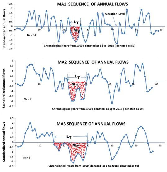
Figure 2 Redistribution of drought lengths and magnitudes with varying MA smoothing.
The MA sequences can be formed from flows or the SHI sequences,
alike. However, it is convenient to apply flow sequences to compute the VR
using SPA, whereas DM based method explicitly requires SHI sequences.
When the annual SHI (or flow) sequence is used without involving any
moving average operations then such a sequence is designated as moving
average 1 (MA1) sequence. In other words, a non-averaged value of SHI (or
flow) is essentially the annual SHI (or flow). When consecutive 2 or 3 or annual
SHIs (or flows) are averaged out then such a running sequence is termed as
MA2 or MA3 sequence. Figure 2 displays MA1, MA2 and MA3 annual SHI
sequences with the drought parameters for the South Saskatchewan River. The
8Preprints (www.preprints.org) | NOT PEER-REVIEWED | Posted: 13 July 2021 doi:10.20944/preprints202107.0301.v1
MA1 sequence (flows) was subjected to analysis to compute the mean (µ),
standard deviation (σ) and lag-1 autocorrelation (ρ). The aforesaid statistics
were also evaluated for the MA2 and MA3 (flows) sequences and are shown
in Table 3. Using the above values of mean and standard deviation, the MA1,
MA2 and MA3 flow sequences were converted to respective SHI sequences.
In the process of analysis, the number of drought spells (Ns) dropped from the
MA1 through MA3 sequences and are presented in column 5 of Table 3. After
a few MA smoothing, Ns attained nearly an equilibrium state and thus
suggesting no further MA smoothing were warranted. For example, in Table
3, Ns values for MA3 smoothing marginally deviate from MA2 but
significantly drop from MA1.
Table 3 Summarized VR (SPA) and DT (DM method -counting) on the MA smoothed annual SHI Sequences.
Computation of Reservoir Volume (m3/s-yr.)
River details MA Mean q Ns σ (m3/s-yr.), ρ DM Method SPA*
number (m3/s) MT-o MT-e ‘DT-o DT- o VR **
1 2 3 4 5 6 7 8 9 10 11
Bow river MA1 39.12 0.48 26 5.18, 0.06 5.84 7.02 30.27 30.27 78.11
N=108(1911-18) MA2 39.10 0.49 15 3.79, 0.57 13.02 13.22 49.35 67.46 --
MA3 39.08 0.51 15 3.23, 0.68 14.52 15.15 47.48 75.23 --
Bow River MA1 38.44 0.52 17 5.12, 0.11 4.98 6.72 25.45 25.45 54.73
N=62(1955-16) MA2 38.48 0.46 10 3.84, 0.57 11.08 10.52 42.53 56.67 --
MA3 38.51 0.53 9 3.25, 0.65 12.20 11.39 39.65 62.44 --
Saskatchewan MA1 167.1 0.51 14 58.83, 0.20 8.86 6.62 521.09 508.59 708.07
River MA2 167.5 0.48 7 45.95, 0.66 10.72 11.09 509. 58 630.68 --
N=59(1960-18) MA3 167.9 0.54 6 40.63, 0.81 13.71 13.07 557.04 806.41 --
Saskatchewan MA1 159.8 0.50 12 60.62, 0.09 4.40 5.88 266.72 266.72 504.28
River MA2 158.4 0.46 6 44.40, 0.53 9.46 8.41 420.20 573.67 --
N=42(1970-11) MA3 157.3 0.43 5 37.11, 0.74 10.39 9.85 385.37 629.53 --
* SPA denotes sequent peak algorithm, ** VR reservoir volume by the closest SPA. The bold letters signify values
.corresponding to VR.
For a comparative analysis on VR, the counting procedure was applied
to the MA1 sequences. The VR (Table 3, column 11 and in the subsequent text)
were computed using SPA for comparison with DT-o. The counting for DT-o was
done in terms of MT-o (SHI sequences, Table 3), which were truncated at the
level of 0 (z0 = 0), then converted to DT-o (DT-o = σ × MT-o). In the MA1 smoothing,
there is only one standard deviation, so after calculating the value of MT-o1, the
value of DT-o1 was obtained using the above relationship by replacing σ with
σ1, i.e. the standard deviation of the MA1 sequence.
9Preprints (www.preprints.org) | NOT PEER-REVIEWED | Posted: 13 July 2021 doi:10.20944/preprints202107.0301.v1
Figure 3 Flow-diagram for computing deficit volumes under various options in the DM method
When the DT-o based on the MA1 analysis did not match or were far less
than the VR, then the analysis was extended to MA2 and at times to MA3
sequences. For the MA2 smoothing, the value of DT-o (denoted as DT-o2) was
obtained using the corresponding value of the standard deviation (denoted by
σ2) and MT-o (say MT-o2), i.e. DT-o2 = σ2 × MT-o2. For further comparison, another
value of DT-o2 was also computed using σ1 (based on MA1 or the original flow
sequence), i.e. DT-o2 = σ1 × MT-o2 (Table 3). Likewise, for the MA3 smoothing, two
values of DT-o3 were obtained; one based on σ3 (DT-o3 = σ3 × MT-o3; σ3 being the
standard deviation obtained after MA3 smoothing) and another value as DT-o3
= σ1 × MT-o3. The aim is to choose the MA smoothing that will provide the best
equivalence of DT-o to VR. The above sequence of computations is portrayed in
a flow diagram (Figure 3). In the flow diagram, the symbols DT-o and MT-o are
denoted by DT and MT for the sake of brevity and ease of writing and they can
also represent DT-e and MT-e with the common multiplier σ1. In the flow
diagram VR’ stands for the standardized value of VR, i.e. = VR/σ1, which
corresponds to MT.
Parallel to the counting procedure, the MT values (denoted as MT-e) were
obtained by using the analytical procedure (Equations 2 and 3). The
corresponding values of DT-e were computed (DT-e = σ1 × MT-e). The VR values
were compared with the values of DT-e. Two values of MT-e were computed for
each situation, i.e. one value using the mean as well as the variance in Equation
(2) and the other value by simply using the mean based on Equation (3), thus
10Preprints (www.preprints.org) | NOT PEER-REVIEWED | Posted: 13 July 2021 doi:10.20944/preprints202107.0301.v1
yielding two values of DT-e. Both the values were compared with VR for
arriving at an appropriate value of DT-e for further analysis and use.
4. Results
4.1. Role of the time scale on the size of reservoirs
To discern the role of the annual, monthly and weekly time scales, VR
(SPA) and DT-o (counting procedure in the DM method) from the respective
flows and SHI sequences were computed and are summarized for 6 rivers in
Table 2. It was found that the values of VR at the aforesaid time scales were
fairly close to each other with a tendency to slightly increase (0 to 20% with an
average value of 10%) at the monthly and weekly scales compared to the
annual scale. The monthly and weekly DT-o values tended to decrease
compared to annual values of DT-o with an average reduction of 25% (range
from 21 to 59%). The other point that emerged from the calculations was that
the VR was greater than DT-o at all-time scales. For example, at the annual scale,
VR values were found to be larger (ranging from 0 to 200%), with an average
of nearly 70%. The reduction in the storage requirement in terms of deficit
volumes makes sense because at monthly and weekly scales the actual
drought periods are estimated more accurately due to time scale effects and
are usually shortened and thus requiring less amount of water to meet the
demand. On the contrary, in the SPA based calculations for VR, the fluctuations
at a shorter time scale would be larger requiring greater reservoir volume to
damp out such fluctuations to meet the constant demand.
The above numbers displaying large discrepancies between the SPA
and DM based (MA1) estimates highlight that either the SPA yields excessive
values of reservoir volume or the DM method yields too small estimates at the
draft level of mean annual flow (MAF, 1µ ). At the annual scale, however,
when the draft was lowered to 0.90µ or less, the estimates by the SPA and DM
method converged to the same value [20]. In other words, a region with a
draft level between 0.90µ and 1µ requires special consideration for the
estimation of reservoir volumes by the DM method. The SPA based estimates
can be construed as fixed with little scope to lower them in view of the inherent
algorithm imbued in it. But the DM based estimates can be boosted by utilizing
the MA procedure to attain parity with SPA based estimates. The SPA has
been in vogue since the 1960s [26] and is universally accepted to design the
reservoir capacity, therefore, the focus in this study is to arrive at a suitable
MA smoothing that should yield DT comparable to VR at the draft level of 1µ.
The DM based estimates (italicized, Table 2) at the monthly and weekly
scales without standardization were found to be slightly different (mostly
smaller) in comparison to the standardization based values (SHI sequences).
11Preprints (www.preprints.org) | NOT PEER-REVIEWED | Posted: 13 July 2021 doi:10.20944/preprints202107.0301.v1
On average, the standardization based estimates were found about 12% larger
than those based on the non-standardized values. This discrepancy can be
perceived to arise because of σav, which has been taken as the representative
value of the standard deviation to convert the magnitude in deficit volume (DT
= σav× MT). Needless to mention that σav is an estimator representing 12 values
of monthly σ’s and is unlikely to be the best for all situations, but is construed
to be a better option compared to other options mentioned earlier. Since
standardization is purely statistical in this operation, the pdf of monthly
sequences is less likely to play the role in explaining the aforesaid discrepancy.
At the annual scale, however, it should be noted that the standard deviation
has only one value, thus estimates by both routes turned out to be identical.
Therefore, only one value of DT-o is reported in Table 2. Since these estimates
(i.e. without standardization) do not require the use of standard deviation in
the calculations and thus can be deemed more accurate. However, the
standardization procedure is better amenable to statistical analysis, and
estimates based on this approach are more conservative (i.e. higher compared
to the non-standardization, Table 2). Based on the foregoing reasoning, the
route involving standardization (i.e., the use of SHI sequences) for the
estimation of DT-o has been preferred in subsequent analyses and the annual
scale is considered as a first choice.
4.2. Comparison of reservoir sizes using the SPA and the DM based counting
procedure
In computing the DT-o, the first step is to choose the right value of σ at each
MA smoothing. For example, in the MA2 smoothing, there are two DT-o: one based
on σ2 (i.e. 'DT-02 = σ2 × MT-o2) and another based on σ1 (i.e. DT-02 = σ1 × MT-o2). For the
MA1 smoothing, there is only one standard deviation and thus DT-o1 = 'DT-o1 (Table
3). It is apparent from Table 3 that 'DT-o values either inconsistently decrease or
increase in MA2 and MA3 smoothing; whereas DT-o values are consistently
increasing and hence σ1 is the crucial parameter to be used for matching to the VR
to arrive at an appropriate MA smoothing. In other words, σ1 must be used as a
multiplier with MT-o in every MA smoothing for estimation of DT-o and the role of σ2
and σ3 is confined to the standardization of the smoothed MA2 and MA3 flow
sequences. It should be noted that for consistency and ease, only 1.0 σ1 is being used
as a multiplier. Other fractions of σ1 (such as 1.2, 1.1, 0.90 or 0.80) were neither
considered nor tested for their efficacy in this study.
In assessing the efficacy of various smoothing, the values of DT-o and VR
were compared on a 1:1 basis and the performance statistics, viz. the Nash-
Sutcliffe efficiency (NSE), and the mean error (MER) were used [27]. To arrive
at the above estimates of performance statistics, values of VR and DT-o were
standardized dividing them by σ1 (MA1). In other words, a 1:1 comparison
12Preprints (www.preprints.org) | NOT PEER-REVIEWED | Posted: 13 July 2021 doi:10.20944/preprints202107.0301.v1
was made between DT-o /σ1 = MT-o and VR /σ1 (denoted by VR'). In doing so, the
wild variation in these entities (i.e. DT-o and VR) from small to large rivers were
homogenized while rendering them non-dimensional, and thus resulting in
sensible estimates of NSE and MER. The efficacy is being tested using NSE
and MER [27] as these statistics have been widely used during the past 50
years and are time tested measures in hydrologic investigations.
Based on aforesaid calculations, it was found that MT-o for MA1
sequences turned out to be significantly less than VR' with a caveat that in a
few cases, the values of MT-o were found to be equal to VR'. In other words, the
values of the MT-o compared poorly with VR' which is also apparent from an
utterly low value of NSE ≈ 24% and MER ≈ -39% (Table 4). In brief, the VR'
tended to be very conservative (meaning larger), whereas DM based
estimates, i.e. MT-o appeared to be significantly smaller. Since the discrepancies
in values of MT-o and the VR' were excessively large, therefore, the MA2 and
MA3 smoothing were considered.
Table 4 Performance statistics for comparison of SPA based VR with DM based DT.
Drought magnitude based analysis
Type of model Performance MA1 MA2 MA3 Average of
statistic MA2 & MA3
Calculations by the counting method NSE (%) 24.33 71.93 69.36 86.73
from the observed flow data MER (%) -38.83 -13.04 17.50 2.23
DM model with consideration of the mean of NSE (%) 25.90 49.08 56.70 53.60
drought intensity only, Equation (3) MER (%) -49.80 -36.30 -26.83 -31.56
DM model with consideration of the mean and NSE (%) 46.23 72.01 65.08 71.02
variance of drought intensity, Equation (2) MER (%) -23.71 0.75 13.85 7.30
Firstly, the MA2 based MT-o2 values were compared to the VR' on a 1:1
basis. It was discovered that with the MA2 smoothing, the matching to VR'
significantly improved resulting in NSE ≈ 72% and MER ≈ -13% (Table 4). In
other words, the underestimation was ameliorated significantly as the value
of MER ascended from -39% to -13%. Although the NSE values have improved
remarkably, there still existed a scope for improvement in the estimates of the
DT-o because underestimation was endemic as revealed by MER of -13%.
Thus, MA3 smoothing was undertaken (flow chart-Figure 3) and values
of MT-o3 were obtained. The MA3 sequences resulted in the over-estimation of
DT-o values with MER = 17.50% although the value of NSE dropped marginally
to 69.36% (Table 4). In short, the MA2 smoothing led to the under-counting
whereas the MA3 smoothing led to the over-counting of the DT-o values with
NSE being nearly the same. For comparison with values of VR, therefore, it was
considered reasonable to average out the DT-o values based on the MA2 and
the MA3 smoothing. Such a comparison was made by plotting the average
13Preprints (www.preprints.org) | NOT PEER-REVIEWED | Posted: 13 July 2021 doi:10.20944/preprints202107.0301.v1
values of the MT-o2 and MT-o3 against the values of VR' and resulted in a
remarkably improved match with NSE ≈ 87% and MER ≈ 2% (Figure 4A, Table
4). The important point to be noted is that at every smoothing, a new value of
MT-o will emerge, which is multiplied by the MA1 smoothing based value of σ
(= σ1) to arrive at the new estimate of DT-o.
Figure 4 Comparison of SPA based VR with (A) MT-o by counting procedure (B) MT by a hybrid procedure
i.e. MT = a bigger value between MT-o and MT-e
In the process of moving from the MA1 smoothing to the MA2
smoothing, there has been a considerable reduction in the number of drought
spells (column 5, Table 3). Such a reduction suggests that there is a significant
increase in the drought length (Figure 2) and in turn, there is also a significant
increase in the drought magnitude. In other words, the smoothing procedure
led to the amalgamation of smaller drought episodes with the larger ones
which resulted in enhanced values of the DT-o (or MT-o). Such enhanced values
have been found to compare well with VR (or VR').
4.3. Comparison of reservoir sizes using the SPA and DM based Model
The drought magnitudes (MT-e) in the standardized domain were
estimated using Equations (2) and (3). At the annual scale, the characteristic
drought length was found equivalent to extreme drought length, L T [12],
obtained from the Markov chain based relationship. In the first version, the
MT-e was estimated by involving only the mean of the drought intensity i.e.
Equation (3) while in the second version, both the mean and variance of
drought intensity were considered i.e. Equation (2) to arrive at estimates of the
MT-e and hence estimates of the DT-e. The calculation for DT-e was done using σ1,
i.e. DT-e = σ1 × MT-e, which is similar to the case of DT-o. Because of similarity, the
best multiplier was σ1 for all MA smoothing in the estimation of DT-e. For
14Preprints (www.preprints.org) | NOT PEER-REVIEWED | Posted: 13 July 2021 doi:10.20944/preprints202107.0301.v1
example, there are two estimates of DT-e (viz. DT-e2 = σ2× MT-e2 and DT-e2 = σ1 ×
MT-e2) if the MA2 smoothing was conducted, then the appropriate value will
be DT-e2 (= σ1 × MT-e2), which, in turn, should be comparable to VR or the
counting based DT-o2. One can advance similar arguments to the MA3
smoothing. Succinctly, σ1 is the multiplier for all MA smoothing chosen for
estimating DT-e in the analytical approach as was the case for DT-o. It was found
that the estimation by a simple version involving only the mean of the drought
intensity proved too inadequate both in terms of NSE and MER. The
calculations showed that values of MT-e are nearly 50% of VR with the MA1
smoothing and such an underestimation persisted even with the MA3
smoothing leading to the value of MER = - 27% (Table 4 ). The NSE for the
MA3 smoothing was also low with the highest value nearly equal to 57%.
Similar was the case for the MA2 smoothing with NSE = 49% and MER = -36%
(Table 4).
In view of the abysmal values of the performance statistics by Equation
(3), Equation (2) was used to estimate MT-e and its corresponding DT-e. The
performance statistics turned out to be encouraging. Although, there was a
significant underestimation (≈ -24%) for the MA1 smoothing, however, the
underestimation improved remarkably (MER= 0.75%) with the corresponding
NSE =72% for the MA2 smoothing. A consideration of MA3 smoothing
resulted in a significant overestimation of nearly 14% and a slight reduction of
NSE to 65%, which suggested that the MA3 smoothing is less meaningful.
However, the estimates of MT-e, based on the MA2 smoothing and the MA3
smoothing were averaged out and the resultant performance statistics
improved compared to those of the MA2 smoothing with an acceptable
overestimation (7.30%). Likewise, the NSE of 71% was almost equal to 72%
that was obtained for the MA2 smoothing. In nutshell, the analytical (model)
approach also yielded estimates of MT-e (or DT-e) which are in agreement with
those of the counting method. However, the analytical procedure proved a bit
rigorous as it involved the numerical integration of relevant equations
reported by Sharma and Panu [12] and the resultant output from which, in
turn, became input into Equation (2).
It was observed that the MA2 smoothing resulted in similar values of
NSE for both the counted DT-o as well as the estimated DT-e (Equation 2). The
counted values of DT-o were ameliorated by averaging the values obtained
from the MA2 and the MA3 smoothing. Such an averaging by the analytical
estimates involving the MA2 and MA3 smoothing resulted in little
improvement over the counted values. At this point, it was mooted that the
MA2 smoothing is preserved and the larger value between DT-o (MT-o) and DT-
e (MT-e) (Table 5) be used as the final estimate of the reservoir volume. For an
evaluation of the performance statistics, viz. NSE and MER, the V R’ and MT
15Preprints (www.preprints.org) | NOT PEER-REVIEWED | Posted: 13 July 2021 doi:10.20944/preprints202107.0301.v1
(larger between MT-e and MT-o) were compared on a 1:1 basis (Table 5, Figure
4B).
Table 5 Summary of the VR', MT-o and MT-e based on the hybrid procedure on MA2 smoothed annual
SHI sequences for the selected rivers.
Counting Method Analytical Method
River name and σ1 MT-o = MT-e = Best VR
Flow data size ρ (m3/s-yr) (DT-o /σ1) DT-e / σ1 DT-e / σ1 MT (m3/s-yr) VR'
(Eq. 3) (Eq. 2)
(1) (2) (3) (4) (5) (6) (7) (8) (9)
Bow River 0.57 5.18 13.02 7.55 13.22 13.22 78.11 15.08
(1911-18) N=108
Bow River 0.57 5.05 11.29 6.37 10.66 10.66 56.73 11.23
(1955-18)N=64
S. Saskatchewan R. 0.66 58.83 10.72 6.73 11.25 11.25 708.07 12.04
(1960-18) N=59
S. Saskatchewan R. 0.53 60.62 9.46 5.30 8.41 9.46 257.52 8.32
(1970-11)N=42
English River 0.58 19.06 9.00 7.39 12.87 12.87 254.72 13.36
(1922-18) N=97
English River 0.51 18.73 11.55 5.64 9.19 11.55 30.44 10.64
(1965-16) N=52
Pagwachaun River 0.40 5.79 4.61 5.17 8.33 5.17⃰⃰ 2.69 5.26
(1968-18) N=51
Bevearbank River 0.30 0.56 4.17 5.45 8.95 5.45⃰ 2.63 4.69
(1922-1997) N=76
Note: *(asterisk) means the value is based by comparing MT-o and MT-e (Equation 3) because of ρ being < 0.42.
The foregoing selection criteria of the larger estimate between the MT-e
and the MT-o (named as hybrid procedure) resulted in the value of NSE about
85% with an acceptable level of overestimation (MER = 4.7%). The criteria
performed well in a majority of rivers except in cases where ρ was found to be
less than 0.42 for the MA2 sequences. In such cases, the value of the MT-e based
on Equation (3) was compared with the estimate of the MT-o and the bigger
value was chosen to represent the reservoir volume. In nutshell, the MA2
smoothing is satisfactory for the evaluation of reservoir volumes at the annual
scale and conversely, a little gain is achieved by invoking higher MA
smoothing, with the caveat that the bigger one between DT-e (= σ1 × MT-e ) and
DT-o (= σ1 × MT-o) should be chosen as the estimator of deficit volume to
correspond with reservoir volume.
5. Discussion
From the foregoing analysis, it was observed, that the discrepancy
between the VR (SPA) and DT (DM) is significant at the draft level of mean
16Preprints (www.preprints.org) | NOT PEER-REVIEWED | Posted: 13 July 2021 doi:10.20944/preprints202107.0301.v1
annual flow when only MA1 smoothing is applied on SHI sequences. The
large discrepancies between the SPA and DM based (MA1) estimates are an
eye-opener in that either the SPA yields too large values of reservoir volume
or the DM method yields too small estimates. No such estimates can be
considered to be absolute as each method has its own logistics and limitations.
In the case of SPA, the difference between the full reservoir level (reservoir is
assumed to be full at the beginning) and the lowest level reached during the
sampling period, is taken as the reservoir volume. During this intervening
period, several droughts including the longest one may occur and the recovery
in the water levels in the reservoir may succeed. Conversely in the DM based
method, no such assumption is invoked and thus the total shortfall of water
below the long term mean flow in a river during the longest drought period is
regarded as the required reservoir volume. The reservoir should be designed
to store the above volume of water during the period of excess flow in the
river.
In a bid to attain the same DT values as VR using the DM based method,
the drought lengths and in turn, the magnitudes were amplified by a moving
average procedure that resulted in the MA2 and MA3 sequences. The DT
values based on the MA2 sequences tend to undercount whereas those based
on the MA3 sequences tend to over count compared to the VR. On an annual
basis, either MA2 or MA3 smoothing can only be conducted because there is
no smoothing operation between these two, i.e. there is no integer number
between MA2 and MA3 smoothing. Therefore, any further refinement of
results stresses that the analysis should be conducted at a shorter time scale
(i.e. the monthly scale). There exists an opportunity for a suitable match
between the VR and DT values, provided MA smoothing such as 3-, 4-, 5-, 6- or
higher monthly SHI sequences are utilized [28]. This is an area for further
research justifying the use of monthly based analysis in the design of
reservoirs.
It turned out that at the demand level at the mean annual flow of a river,
the VR values tend to be not significantly different from each other irrespective
of what time scale is chosen. In contrast, the drought magnitude based method
resulted in significant discrepancy among these estimates (DT) with the annual
time scale yielding much higher values compared to those at the monthly and
weekly scales. In such a scenario, one can even be tempted to limit the analysis
to the annual flow sequences only as it is trivial and the annual flow data can
easily be synthesized or generated at any desired location on a river. The aim
is to store enough water to meet any exigency or unaccounted episodes. There
is also a need to examine other methods of estimating the reservoir capacity
and compare them with the DM based estimates. Finally, all the estimates may
be averaged out to arrive at the final design value of the reservoir capacity.
17Preprints (www.preprints.org) | NOT PEER-REVIEWED | Posted: 13 July 2021 doi:10.20944/preprints202107.0301.v1
6. Conclusions
The analysis was carried out to compare the VR and DT respectively,
using the SPA and the DM based method (counting and analytical procedures)
on the flow data from 15 rivers across Canada. The estimates of VR at the
annual, monthly and weekly scales with the draft set at the mean annual flow
level were observed close to each other with a tendency to slightly increase at
the monthly and weekly scales. On the contrary, estimates of DT at monthly
and weekly scales tended to decrease compared to the annual scale. At all
three time scales, the DT estimates turned out to be smaller than VR. To
ameliorate the DT to the level of VR, the counting and analytical procedures (in
the DM based Method) were applied to flow and SHI sequences on an annual
scale. In the counting procedure, the best parity was found with the averaged
out values of DT-o that were obtained by MA2 and MA3 smoothing of SHI
sequences. Likewise, the analytical procedure yielded similar results (in terms
of DT-e) when applied on MA2 and MA3 smoothed SHI sequences. In the
analytical procedure, the relationships were built on the extreme number
theorem, the truncated normal probability distribution of the drought
intensity, normal distribution of the drought magnitude and a Markov chain
based value of extreme drought length. The estimation of DT-e was found
inadequate when only the mean of the drought intensity was used. The
consideration of the mean and the variance of the drought intensity in the
analytical procedure turned out to be satisfactory and corroborated the results
obtained from the counting procedure. Another finding of the study was that
the MA2 smoothing of SHI sequences is sufficiently provided that the larger
value between DT-o and DT-e is taken as a counterpart value of the reservoir
volume for design purposes. The novel feature of the DM method lies in its
ability to assess the reservoir volume without assuming the reservoir being
full at the beginning of the analysis as is the case with SPA. Further, the DM
based method is capable of considering the return period and associated risk
in the design process of reservoirs. However, the DM method requires flow
sequences to be stationary unlike the SPA, which applies to stationary and
nonstationary flow sequences alike. It is recommended that the study be
extended to the monthly scale at varying draft levels such as 80%, 70%, 60%,
50% etc. of the mean annual flow, which are largely used where environmental
concerns are the overriding factors in the design of reservoirs across the globe.
Acknowledgements
The partial financial support of the Natural Sciences and Engineering
Research Council of Canada for this paper is gratefully acknowledged.
18Preprints (www.preprints.org) | NOT PEER-REVIEWED | Posted: 13 July 2021 doi:10.20944/preprints202107.0301.v1
Disclosure statement
No potential conflict was reported by the author(s).
References
1. Stedinger, J.R.; Vogel, R.M.; Foufoula-Georgia, E. Frequency analysis of extreme events. Chapter 18, In Maidment
D.R. (ed.) Handbook of Hydrology, New York: Mc-Graw Hill,.1993
2. Tallaksen, L.M.; Madsen, H.; Clausen, B. On the definition and modeling of streamflow drought duration and deficit
volume. Hydrol. Sci. J. 1997, 42(1), 15-33.
3. Tallaksen, L.M.; Van Lanen, H.A. (editors). Hydrological Drought: Processes and Estimation Methods for Streamflow
and Groundwater, Developments in Water Science Vol.48. Elsevier, Amsterdam, Netherlands.2004.
4. Fleig, A.K.; Tallaksen, L.M.; Hisdal, H.; Demuth, S. A global evaluation of streamflow drought characteristics.
Hydrol. Earth Syst. Sci. 2006, 10, 535-552.
5. Yevjevich, V, Methods for determining statistical properties of droughts, In: Coping with droughts; Yevjevich, V., da
Cunha, L., Vlachos, Eds; Water Resources Publications; Littleton, CO, USA,1983; pp. 22-43.
6. Horn, D.R., 1989. Characteristics and spatial variability of droughts in Idaho. ASCE J. Irrigation and Drainage Eng.,
1989, 115 (1), 111-124.
7. Sen, Z. Statistical analysis of hydrological critical droughts. ASCE J. Hydraul. Eng. 1980, 106(HY1, 99-115.
8. Sen, Z. Applied Drought Modelling, Prediction and Mitigation, Elsevier Inc. Amsterdam, 2015.
9. Zelenhasic, E.; Salvai, A., 1987. A method of streamflow drought analysis. Water Resources Research, 1987, 23(1), 156-
158.
10. Salas, J.; Fu, C.; Cancelliere, A.; Dustin, D.; Bode, D.; Pineda, A.; Vincent, E. 2005. Characterizing the severity and
risk of droughts of the Poudre River, Colorado. Journal of Water Resources Management, 2005, 131(5), 383-393.
11. Akyuz, D.E.; Bayazit, M.; Onoz, B. Markov chain models for hydrological drought characteristics. J. of Hydrometeor.
2012, 13(1), 298-309. doi:10.1175/JHM-D-11-019.127.
12. Sharma, T.C.; Panu, U.S. A semi-empirical method for predicting hydrological drought magnitudes in the Canadian
prairies. Hydrological Sciences Journal, 2013, 58 (3), 549-569.
13. Sharma, T.C.; Panu, U.S. Modelling of hydrological drought durations and magnitudes: Experiences on Canadian
streamflows. Journal of Hydrology: Regional Studies, 2014, 1, 92-106.
14. Shukla, S.; wood, A.W. Use of a standardized runoff index for characterizing hydrologic drought. Geophysical
Research Letters, 2008, 35, L02405,doi:10.1029/2007GL032487,2008
15. Nalbantis, I.; Tsakiris, G., 2009. Assessment of hydrological drought revisited. Water Resources Management, 2009,
23, 881-897.
16. McKee, T.B.; Doesen, N. J.; Kleist, J. The relationship of drought frequency and duration to time scales. Preprints,
8th Conference on Applied Climatology, 17-22 January, Anaheim, California, USA, 179-184.1993.
17. Vicente-Serrano, S.M.; Lopez Moreno. Hydrological response to different time scales of climatological drought: an
evaluation of the standardized precipitation index in a mountainous Mediterranean basin. Hydrology and Earth
System Science, 2005, 9, 523-533.
18. Barker, K.J.; Hannaford, J.; Chiverton, A.; Stevenson, C. From meteorological to hydrological droughts using
standardized indicators. Hydrology and Earth System Science. 2016, 20, 2483-2505.
19. Sharma, T.C.; Panu, U.S. Reservoir sizing at draft level of 75% of mean annual flow using drought magnitude based
method on Canadian Rivers. American Institute of Hydrology journal Hydrology, 2021,
8,79.https://doi.org/103390/hydrology8020079.
20. Sharma, T.C.; Panu, U.S. A drought magnitude based-method for reservoir sizing: a case of annual and monthly
flows from Canadian rivers. Journal of Hydrology: Regional Studies, 2021, 36, 100829.
21. Linsley, R.K.; Franzini, J.B.; Freyburg, D.L.; Tchobanoglous, G. Water Resources Engineering, 4th edition, Irwin
McGraw-Hill. New York, 1992, p.192.
22. McMahon, T.A.; Adeloye A.J. Water Resources Yield. Water Resources Publications, Littleton, Colorado, 2005.
23. Dracup, J.A.; Lee, K.S.; Paulson, Jr., E.G. On the statistical characteristics of drought events. Water Resources
Research, 1980, 16(2), 289-296.
19Preprints (www.preprints.org) | NOT PEER-REVIEWED | Posted: 13 July 2021 doi:10.20944/preprints202107.0301.v1
24. Todorovic, P.; Woolhiser, D.A. A stochastic model of n day precipitation. Journal of Applied Meteorology, 1975,
14,125-127.
25. Environment Canada, HYDAT CD-ROM Version 96-1.04 and HYDAT CD-ROM User’s Manual. Surface Water
and Sediment Data Water Survey of Canada. 2018.
26. Thomas, H.A.; Burden, R.P. Operation Research in Water Quality Management. Division of Engineering and Applied
Physics, Harvard University, USA, 1963.
27. Nash, J.E.; Sutcliffe, J.V., 1970. River flow forecasting through conceptual models: part 1, A discussion of
principles, Journal of Hydrology, 1970, 10(3), 282-289.
28. Vicente-Serrano, S.M. Differences in spatial patterns of drought on different time scales: An analysis of the Iberian
Peninsula. Water Resour. Manag. 2006, 20, 37-60.
20You can also read