Non-trivial quantum oscillation geometric phase shift in a trivial band
←
→
Page content transcription
If your browser does not render page correctly, please read the page content below
Non-trivial quantum oscillation geometric phase shift in a trivial band
                                                               Biswajit Datta,1 Pratap Chandra Adak,1 Li-kun Shi,2 Kenji Watanabe,3 Takashi Taniguchi,3 Justin C. W.
                                                               Song,2, 4 and Mandar M. Deshmukh1, a)
                                                               1)
                                                                  Department of Condensed Matter Physics and Materials Science, Tata Institute of Fundamental Research,
                                                               Homi Bhabha Road, Mumbai 400005, Indiab)
                                                               2)
                                                                  Institute of High Performance Computing, Agency for Science, Technology, & Research,
                                                               Singapore 138632
                                                               3)
                                                                  National Institute for Materials Science, 1-1 Namiki, Tsukuba 305-0044, Japan
                                                               4)
                                                                  Division of Physics and Applied Physics, Nanyang Technological University,
                                                               Singapore 637371
arXiv:1902.04264v2 [cond-mat.mes-hall] 13 Feb 2019

                                                               The accumulation of non-trivial geometric phases in a material’s response is often a tell-tale sign of a rich
                                                               underlying internal structure1–3 . Studying quantum oscillations provides one of the ways to determine these
                                                               geometrical phases, such as Berry’s phase4–6 , that play a central role in topological quantum materials.
                                                               We report on magneto-transport measurements in ABA-trilayer graphene, the band structure of which is
                                                               comprised of a weakly gapped linear Dirac band, nested within a trivial quadratic band7–9 . Here we show
                                                               Shubnikov-de Haas (SdH) oscillations of the quadratic band shifted by a phase that sharply departs from the
                                                               expected 2π Berry’s phase. Our analysis reveals that, surprisingly, the anomalous phase shift is non-trivial
                                                               and is inherited from the non-trivial Berry’s phase of the linear Dirac band due to strong filling-enforced
                                                               constraints between the linear and quadratic band Fermi surfaces. Given that many topological materials
                                                               contain multiple bands, our work indicates how additional bands, which are thought to obscure the analysis,
                                                               can actually be exploited to tease out the subtle effects of Berry’s phase.

                                                        Non-trivial geometric phases can arise from diverse             Here we unveil a new phase shift for quantum oscilla-
                                                     settings including in strong spin-orbit coupled systems         tions that appears in multi-Fermi-surface metals. In par-
                                                     that possess real-space10,11 or momentum-space spin-            ticular, we reveal how the quantum oscillations of a com-
                                                     texture12 , periodic driving by strong electromagnetic          pletely trivial Fermi surface (with a constant and trivial
                                                     fields13 , and multi-orbital/site structure within a unit       Berry’s phase) can acquire non-trivial (±π) phase shifts
                                                     cell14 . Even though such phases are often encoded in the       that are gate-tunable. The anomalous phase shifts are
                                                     subtle twisting of electronic wavefunctions, their impact       found in measured SdH oscillations of a trivial band in
                                                     on material response can be profound, being responsible         a multi-band system – ABA-trilayer graphene – and, as
                                                     for a wealth of unconventional quantum behaviors that           we discuss below originate from strong filling-enforced-
                                                     include unconventional magneto-electric coupling15 , an         constraints among Fermi surfaces that unavoidably arise
                                                     emergent electro-magnetic field for electrons11 , and pro-      in multi-Fermi-surface metals. Our experiment probes
                                                     tected edge modes16 amongst others.                             for the first time the continuous variation of the Berry’s
                                                        A prominent example is the Berry’s phase4–6 . In             phase induced quantum oscillation phase shift, as a func-
                                                     anomalous Hall metals, the Berry’s phase on the Fermi           tion of gate voltage (VBG ), in an inversion symmetry bro-
                                                     surface determines the (un-quantized part of the) anoma-        ken system close to the band edge.
                                                     lous Hall conductivity17,18 ; non-trivial π Berry’s phase
                                                     enforces the absence of back-scattering in topological ma-         We study a high mobility hexagonal boron nitride
                                                     terials19 . Indeed, the value of the Berry’s phase of elec-     (hBN) encapsulated ABA-stacked trilayer graphene de-
                                                     trons as they encircle a single, closed Fermi surface can       vice (see Supplementary Materials I). A metal top gate
                                                     be used as a litmus-test for topological bands — π in-          and a highly doped silicon back gate ensure independent
                                                     dicates a non-trivial band20–24 , whereas 2π indicates a        tunability of charge carrier density and electric field. All
                                                     trivial band25–27 . In the presence of a magnetic field (B),    the measurements are done with a low-frequency lock-
                                                     the (quantized) size of closed cyclotron orbits depends         in technique at 1.5 K. ABA-trilayer graphene is very
                                                     on both the magnetic flux threading the orbits as well          interesting because it is the simplest system support-
                                                     as the Berry’s phase of electrons. As a result, quantum         ing the simultaneous existence of a monolayer graphene
                                                     oscillations of a closed Fermi surface can acquire phase        (MLG)-like linear and a bilayer graphene (BLG)-like
                                                     shifts – a direct result of the Berry’s phase of electrons3 .   quadratic band in experimentally accessible Fermi en-
                                                     This is visible in oscillations of both resistance and ther-    ergy (see Fig. 1a)8,33 . Broken inversion symmetry in
                                                     modynamic quantities like magnetization. Tracking such          ABA-trilayer graphene generates a small mass term in
                                                     quantum oscillations phase shifts have emerged as a pow-        the Hamiltonian8,33 . As a result, both the pairs of bands
                                                     erful probe for topological materials28–32 .                    are individually gapped as seen in Fig. 1a; the band gap
                                                                                                                     of the MLG-like Dirac cone34 is ∼1 meV. Fig. 1a shows
                                                                                                                     that when both these bands are filled, the Fermi sur-
                                                                                                                     face of the ABA-trilayer graphene consists of two Fermi
                                                     a) deshmukh@tifr.res.in
                                                                                                                     contours– the inner contour (smaller in size) comes from
                                                     b) biswajit.datta@tifr.res.in
                                                                                                                     the MLG-like band and the outer contour (larger in size)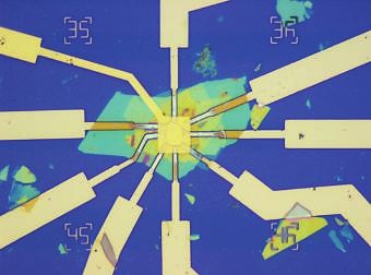
2

                            Kx a                                             graphene, and ΦB is the Berry’s phase. Fig. 2a shows36
     a                        0.00 -0.05
                                                   b                         our measured SdH oscillation in Gxx as a function of

                                                        Energy (meV)
                       0.05
                                                                             B and VBG . The corresponding band structure at zero
                                                                       50    magnetic field is shown in Fig. 2b. Fig. 2c shows an SdH
                     50                                                      oscillation with two distinct frequencies which reveal that
                                                                             two distinct Fermi surfaces are involved in the transport.
                                                                             Fig. 2a is composed of many such SdH oscillation slices
                                                                             at different gate voltages. Theoretically calculated LL di-
      Energy (meV)

                                                                             agram (Fig. 2d) shows that √ the MLG-like and the BLG-
                                                                             like LLs disperse as ∼ B and ∼ B respectively8,9,33 .
                      0                                                      This distinct dispersion of the LLs along with the corre-
                                                                             sponding Hall conductance enable easy identification of
                                                                             the MLG-like and the BLG-like LLs9,34,37,38 .
                                                                                The central result of our study – that of an anomalous
                                                                       -50
                                                                             phase shift in the trivial BLG-like band – is vividly illus-
                                                                             trated in Fig. 2e. It shows three slices of BLG-like SdH
                     -50                            −2π      0     2π
                                                   Berry’s phase             oscillations at different densities away from the crossing
                                                   of the individual         points which correspond to Fermi levels in the valence
                                                   bands                     band, in the gap, and in the conduction band of the
                           0.05
                                                                             MLG-like Dirac cone respectively. We emphasize that
                                   0.00
                                                                             for all these three densities, the Fermi levels lie in the
                                   K ya    -0.05
                                                                             conduction band of the BLG-like band. The SdH oscil-
                                                                             lations above and below the gap clearly show a π phase
FIG. 1. Band diagram of ABA-trilayer graphene. (a) Band                      shift from the SdH oscillation at the gap. This is surpris-
diagram of ABA-stacked trilayer graphene showing one pair of the             ing since the BLG-like band in this energy range has a
conical band (colored red) and another pair of the quadratic band            constant trivial Berry’s phase (see Fig. 1b).
(colored green). Fermi surface at three different energies is overlaid
                                                                                We quantify the anomalous phase shift via a detailed
for which Fermi energy lies in the valence band, band gap and in
the conduction band of the MLG-like band. There is no contour
                                                                             analysis of the SdH oscillations using the standard ex-
from the MLG-like band when Fermi energy is in the band gap. (b)             trapolation method21 . Briefly, this involves fitting a line
Calculated Berry’s phase plot with same color codes for both the             to the LL index (N) corresponding to a minimum in the
bands. Since the bands are gapped, Berry’s phase of the individual           Gxx vs. the corresponding inverse magnetic field ( B1N )
bands goes to zero at the respective band edges.                             plot and examining the intercept at B1 = 0. The method
                                                                             of determining LL indices is described in Supplementary
                                                                             Materials II). From the intercept in the LL index axis
comes from the BLG-like band. Fig. 1b shows that the                         (Fig.3a), we see that the intercept is 0.5 (-0.5) in the
MLG-like Dirac cone has a robust π Berry’s phase which                       valence (conduction) band and is zero in the middle of
only reduces to zero in the vicinity of the MLG-like band                    the band gap. The 0.5 (-0.5) value of the intercept cor-
edge. On the other hand, the BLG-like conduction band                        responds to a π (-π) phase shift of the SdH oscillations
has more-or-less a constant trivial Berry’s phase 2π in                      when the Fermi level lies away from the band gap even
the region of interest (around the Dirac cone gap). In                       though the phase is extracted only from the BLG-like
our experiment, we probe a narrow energy window near                         SdH oscillations. Fig.3b shows fits at several densities
the MLG-like band gap. In the following, we use “band                        away from the gap (firmly in either conduction or valence
gap” to refer to the MLG-like Dirac cone gap.                                band). While possessing different slopes, their intercepts
                                                                             assume only two quantized values: 0.5 or -0.5 depend-
   In the presence of a magnetic field, the continuous band                  ing on the Fermi energy inside the valence or conduction
structure shown in Fig. 1a splits into Landau levels (LLs).                  MLG-like Dirac cone. This reinforces the robustness of
The closed orbits ~k space area takes on quantized values                    the anomalous phase shift.
that depend on the Berry’s phase (and magnetic flux).                           Strikingly, it is only when the Fermi energy is tuned
As the magnetic field is swept and the charge density is                     through the MLG-like band’s gap, that the intercept
varied independently, LLs cross the Fermi surface giv-                       varies continuously from 0.5 to -0.5, see Fig.3c. We note
ing rise to the density of states oscillations that result                   the smooth gate-tuning through the bandgap is possi-
in longitudinal conductance (Gxx ) oscillations35 . At a                     ble due to the gapless nature of the BLG-like conduction
fixed density, the conductance oscillations (SdH) can be                     bands throughout the region of interest. Both the non-
written as ∆Gxx = G cos[2π( BBF + γ)] where G is the                         trivial values and tunable nature of the anomalous phase
oscillation magnitude, BF = nge   Sh
                                     is the SdH oscillation                  shift sharply departs from the traditional understanding
frequency in 1/B parameter space and the phase shift                         of quantum oscillation being purely sensitive to the spe-
γ = Φ2πB − 12 . Here, nS is the density in S sub-band for a                  cific Fermi surface it is sampling – BLG-like band in the
multiband system, g is the LL degeneracy which is 4 for                      present case.
3
0+B 1+B 0-B 1-B
a 4.5
d -4B -3B -2B 2B 3B 4B 5B
4.0 4
νΤ = -6 2 6 14 18 22
−4 −1 2
3.5 2
log( G x x /( e /h) )
MLG-like K+
MLG-like K-
3.0 3 BLG-like K+
BLG-like K-
B (T)
B (T)
2.5
2 -1M
2.0
-2M 0M
1.5 1M
1
-40 -20 0 20 40
1.0
LL energy (meV)
0.5 e
−30 −20 −10 0 10 20 30
V B G (V)
b
G x x ( e 2 /h)
5
V B G (V)
k y a (10− 2 )
e2 16.0
0
h 9.5
6.5
−5
−40 −20 0 20 40 12 16 20 24 28 32
Energy (meV) Filling factor
c VBG = − 44 V
4
R x x ( Ω)
2
0
0.5 1.0 1.5 2.0 2.5 3.0
B − 1 ( T− 1 )
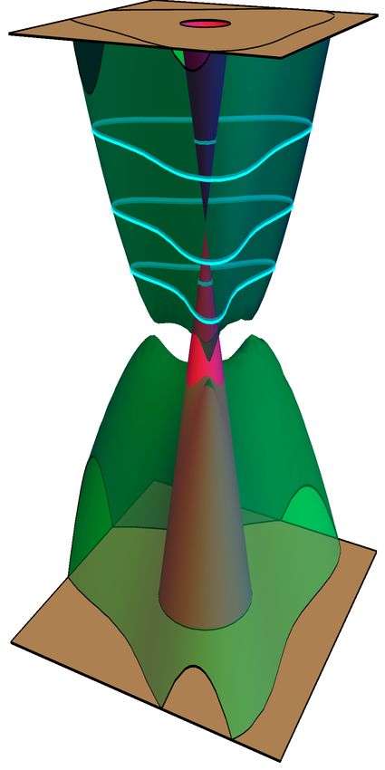
FIG. 2. Magnetotransport of ABA-trilayer graphene. (a) Colour scale plot of Gxx as a function of back gate voltage and
magnetic field. The vertical feature parallel to the magnetic field axis at VBG ∼ 10 V corresponds to the LL crossings of NM =0 LL with
other BLG-like LLs. This VBG also corresponds to the band gap of the MLG-like bands. (b) Energy band diagram shown in the same
energy range as the experimental fan diagram shown in panel (a). (c) An SdH oscillation line slice showing the beating pattern due to
the two bands with different Fermi surface areas. Low and high-frequency oscillations come from the MLG-like and the BLG-like bands
respectively. (d) Theoretically calculated LL energies of the spin degenerate Landau levels as a function of magnetic field. Red and green
lines denote LLs originating from the Dirac and the quadratic bands respectively. Solid and dashed lines denote LLs from K+ and K−
valleys respectively. (e) SdH oscillations (Gxx ) as a function of filling factor below the band gap (green), in the band gap (red) and above
the band gap (blue) which show that the phase of the SdH oscillation in the band gap is π shifted compared to the other two. The curves
are shifted in the vertical direction for clarity. Gate voltage and approximate energy locations of the three SdH oscillation slices are marked
with dashed lines of corresponding color in the fan diagram (a) and in the bandstructure (b) respectively.
We now focus on the origin of the anomalous phase 2 T) even at small magnetic fields. In contrast, the LL
shift. In general, SdH oscillations depend on contribu- spacing of BLG-like LLs is far smaller (∼5 meV at 2 T).
tions from the Fermi surfaces of both the bands: ∆Gxx = This means that multiple BLG-like LLs can be swept
GM cos[2π( BB FM
+ γM )] + GB cos[2π( BBFB + γB )], where M through (over large density and magnetic field windows)
and B subscripts denote MLG-like and BLG-like bands while keeping the filling of the MLG-like LLs constant
respectively. As we explain below, the complex pattern in our experiment, see Fig.2d. This is most prominent
of band fillings across multiple bands of distinct type (en- between the NM = 0 and NM = 1 MLG-like LLs, where
coded in (BFB , BFM )) control the SdH oscillations. we were able to easily resolve and analyze ∼10 BLG-
To unravel the pattern in ABA-trilayer graphene, there like LLs. Even though the filling factor of the BLG-
are two key effects to understand. First, MLG-like LLs like LLs steadily varies over this region, the filling factor
possess large LL separation (first LL gap is ∼50 meV at of the MLG-like band remains pinned to 2 due to the4
a 8.0 2
4.0 1
Landau level index ( N B )
V B G = 16.0 V
-0.5 0
8.0 2
G x x ( e 2 /h)
4.0 1
-0.0 V B G = 9.5 V
0
8.0 2
4.0 1
0.5 V B G = 6.5 V
0
0.0 0.4 0.8 1.2
B − 1 ( T− 1 )
b 10.0
c
8.0
8.0
Landau level index ( N B )
Landau level index ( N B )
6.0
6.0
4.0
4.0 V B G (V)
11.2
V B G (V) 2.0 10.5
2.0
20.0 7.0 9.5
0.5 16.0 6.5 0.5 8.3
12.0 6.0 7.6
−0.5 −0.5
0.0 0.4 0.8 1.2 0.0 0.4 0.8 1.2
B − 1 ( T− 1 ) B − 1 ( T− 1 )
FIG. 3. Anomalous SdH phase shift. (a) SdH oscillations (Gxx ) and the LL index vs inverse magnetic field fit below the band gap
(green), in the band gap (red) and above the band gap (blue). Circles and squares denote the SdH minima and maxima respectively. Inset
of all the panels shows the band diagram and the Fermi energy locations for which the SdH fits are shown. (b) LL index vs inverse magnetic
field fits at different densities away from the band gap. The linear fit produces ± 12 intercept when Fermi level lies in the MLG-like valence
band and MLG-like conduction band respectively. (c) LL index vs inverse magnetic field fits at different densities close to the band gap.
This shows that the intercept varies continuously from 1/2 to -1/2 when the Fermi level goes from the valence to the conduction MLG-like
band by tuning the density. Inset shows the zoomed-in band diagram very close to the band gap.
particularly large first MLG-like LL energy spacing and the MLG-like band. Crucially, for E(0M ) < EF < E(1M )
the non-field-dispersive nature of the NM = 0 LL. As a (above the MLG-like band gap) only NM =0 electron like
result, in between MLG-like LLs [for e.g., that realized in LL is filled, so the filling factor of the MLG-like band
the region E(0M ) < EF < E(1M )] MLG-like oscillations remains pinned to 2. This yields a BLG-like oscilla-
are frozen, and the the SdH oscillations are dominated tion frequency as BBFB = BBFT − 1/2. Similarly, for E(-
by the BLG-like band: ∆Gxx ≈ GB cos[2π( BBFB + γB )]. 1M ) < EF < E(0M ) (below the MLG-like band gap) the
Second, in SdH oscillation measurements, the total filling factor of the MLG-like band remains pinned to -2
density is fixed (set by the gate voltage) while the mag- producing BBFB = BBFT + 1/2. Incorporating both cases
netic field is varied. In ABA-trilayer graphene, the total into the BLG-like SdH oscillations, we obtain
density (nT = nM + nB ) is comprised of the individual
BFT
band densities in each of the MLG-like (nM ) and the ∆Gxx ≈ GB cos[2π( + γB ± 1/2)], (1)
BLG-like (nB ) bands, which may reconfigure with the B
magnetic field while keeping nT constant. This constraint that displays an anomalous, non-trivial, and tunable
strongly influences the BLG-like SdH oscillations. To see phase shift, acquired due to the strong filling-enforced
this we express its oscillation frequency in terms of the constraint above and below the bandgap. This yields
total density via: BFB = n4eBh
= (nT −n
4e
M )h
= BFT − νM4B , an additional π (−π) phase shift in the BLG-like oscil-
nT h nM h
where BFT = 4e and νM = eB is the filling factor of lations due to the fully-emptied (fully-filled) MLG-like5
a 3.0 b 1.25
n = 4 e B FT /h
−4 −1 2 1.20 nT = nM + nB
2.5
log( G x x /( e 2 /h) ) n B = ν B e B /h
n M = ν M e B /h
B (T)
2.0 1.15
Extracted density (1 0 1 2 cm− 2 )
1.10
1.5
1.05
1.0
6 10 14 18 22
V B G (V) 1.00
νM = − 2 − 2 < νM < 2 νM = 2
c (Const) 0 M partially filled (Const) 0.95
12 ( ν B , νM)
π
Phase (Intercept × 2π)
0.90 (16, 2)
Increasing B
(20, 2)
(24, 2)
B FT (T− 1 )
0 8
0.125
Increasing B
0.100
-π
4
0.075
6 10 14 18 15 16 17 18 19 20
VBG (V) V B G (V)
FIG. 4. Comparing the band specific density and the extracted density from the fits. (a) Zoomed in measured LL fan
diagram showing three lines drawn for three filling factors along which we extract the density. (b) MLG-like band density (nM = νM eB/h)
and BLG-like band density (nB = νB eB/h) are marked with filled circle and dash respectively for total filling factor νT =18 (red), 22
(green) and 26 (blue). The unfilled circles of corresponding colors show the total density nT = nM + nB for each total filling factors.
Surprisingly, at a constant gate voltage with increasing magnetic field density of the MLG-like and the BLG-like band increases and
decreases respectively, keeping total density constant at all magnetic fields (filling factors). The black line shows the density calculated
from the SdH frequency (nT = 4e h
× BFT ) which is identical to the combined density for all filling factors. (c) Intercept (blue) and slope
(red) of the BLG-like SdH oscillation fit as a function of VBG . Fitting errors are shown for the intercept. Corresponding band diagram
is overlaid for visualization. Three regions are shaded with three different colors – green shade and blue shade indicate completely empty
and completely filled NM =0 LL respectively whereas the saffron shade indicates partially filled NM =0 LL. This observed phase variation
enables us to directly visualize the population/depopulation of the NM =0 LL.
lowest NM = 0 LL. We have also extracted this phase the bands are νB = 16, 20, 24 whereas νM = 2, obtained
from the theoretically calculated density of states which directly from Hall conductance measurements, see Sup-
supports our experimental finding (see Supplementary plementary Materials. Strikingly, BLG-like band density
Materials III and IV). In general, the filling enforced nB on these lines decrease with the magnetic field (col-
phase of the BLG-like SdH oscillations can be extracted ored dash plots in Fig. 4b); in contrast, MLG-like band
when multiple LLs from the MLG-like bands are filled density in this region increases with the magnetic field
(see Supplementary Materials V). (colored filled circles). These opposite sign variations are
The filling-enforced constraint is further corroborated exactly compensated in their sum nT = nM + nB (see
by the measured quantum oscillation frequency. In par- colored unfilled circles) which is fixed as a function of
ticular, Eq. (1) indicates that the BLG-like quantum os- the magnetic field as evidenced by the collapse of the nT
cillations have 1/B frequency that scale with the com- plots on each other — a demonstration of the intricate re-
bined density of the MLG-like and the BLG-like bands; configuration of density between MLG-like and BLG-like
their sum – the total density – is set globally by the bands.
gate voltage. We will illustrate this by focussing on the Perhaps most dramatic is the precise agreement of the
region between NM = 0 and NM = 1 MLG-like LLs. oscillation frequency BF directly extracted from the mea-
To proceed, we first note that the density in each of the sured SdH oscillations (equivalent density shown as a
bands depends on both filling factor νB,M and B. On Hall solid black line in Fig. 4b) and the sum of densities from
plateaus, the filling factor takes on precise quantized val- the filling factors in each band (colored unfilled circles).
ues, e.g., on the solid lines in Fig. 4a the filling factors in This concordance is expected directly from Eq. (1). To-6
gether with the anomalous phase shift, these empirically and J. C. W. S did the calculations. K.W. and T.T. grew
display the strong effect of the filling-enforced-constraints the hBN crystals. B.D., P.C.A, J. C. W. S and M.M.D.
present in our devices. wrote the manuscript. M.M.D. supervised the project.
Anomalous filling-enforced phases become most pro-
nounced when the quantum oscillations of component 1 D.
Fermi surfaces are resolved simultaneously over a similar Xiao, M.-C. Chang, and Q. Niu, Rev. Mod. Phys. 82, 1959
(2010).
range of magnetic fields. In ABA-trilayer graphene the 2 J. G. Analytis, R. D. McDonald, S. C. Riggs, J.-H. Chu, G. Boe-
BLG-like band has a Fermi surface area that is about binger, and I. R. Fisher, Nature Physics 6, 960 (2010).
3 G. P. Mikitik and Y. V. Sharlai, Physical Review Letters 82, 2147
10 times larger than that of the MLG-like band (at
VBG =-44V), enabling oscillations of both bands to oc- (1999).
4 S. Pancharatnam, in Proc. Indian Acad. Sci. A, Vol. 44 (1956) p.
cur side-by-side (Fig.2c). The anomalous (non-trivial)
247.
phase shifts, that we find in BLG-like bands, amount to 5 M. V. Berry, Proc. R. Soc. Lond. A 392, 45 (1984).
a “proximity”-effect for the phase of quantum oscillations. 6 I. A. Luk’yanchuk and Y. Kopelevich, Phys. Rev. Lett. 93, 166402
To test this, we extracted the phase shift (of the BLG- (2004).
7 T. Taychatanapat, K. Watanabe, T. Taniguchi, and P. Jarillo-
like quantum oscillations) over a fine grid as gate-voltage
Herrero, Nature Physics 7, 621 (2011).
is tuned through the bandgap, see Fig.4c. This displays 8 M. Serbyn and D. A. Abanin, Physical Review B 87, 115422
the smooth evolution of phase shift from π → 0 → −π (2013).
that closely tracks the smooth evolution of Berry’s phase 9 B. Datta, S. Dey, A. Samanta, H. Agarwal, A. Borah, K. Watan-
expected for the gapped MLG-like band in inversion sym- abe, T. Taniguchi, R. Sensarma, and M. M. Deshmukh, Nature
metry broken ABA-trilayer graphene. Given that in typ- Communications 8, 14518 (2017).
10 S. Mühlbauer, B. Binz, F. Jonietz, C. Pfleiderer, A. Rosch,
ical inversion symmetry broken systems, the change of A. Neubauer, R. Georgii, and P. Böni, Science 323, 915 (2009).
Berry’s phase is concentrated close to the band edge 11 N. Nagaosa and Y. Tokura, Nature nanotechnology 8, 899 (2013).
precisely where the number of quantum oscillations is 12 B. A. Bernevig and T. L. Hughes, Topological insulators and
few, “proximity” detection (from a co-existent band with topological superconductors (Princeton university press, 2013).
13 N. H. Lindner, G. Refael, and V. Galitski, Nature Physics 7, 490
more oscillations) can provide a surprising new facility to
(2011).
probe non-trivial quantum geometry. Our studies could 14 D. Xiao, W. Yao, and Q. Niu, Physical Review Letters 99,
shed light also on other topological materials like Weyl 236809 (2007).
semimetals39 that host multiple bands. 15 J. Lee, Z. Wang, H. Xie, K. F. Mak, and J. Shan, Nature mate-
rials 16, 887 (2017).
16 S. Ryu and Y. Hatsugai, Physical Review Letters 89, 077002
(2002).
ACKNOWLEDGEMENTS: 17 F. Haldane, Physical Review Letters 93, 206602 (2004).
18 N. Nagaosa, J. Sinova, S. Onoda, A. H. MacDonald, and N. P.
We thank Jainendra Jain, Allan MacDonald, Sreejith Ong, Rev. Mod. Phys. 82, 1539 (2010).
19 T. Ando, T. Nakanishi, and R. Saito, Journal of the Physical
GJ, Umesh Waghmare, Shamashis Sengupta and Sajal Society of Japan 67, 2857 (1998).
Dhara for helpful discussions. Biswajit Datta is a recip- 20 K. S. Novoselov, A. K. Geim, S. V. Morozov, D. Jiang, M. I.
ient of Prime Minister’s Fellowship Scheme for Doctoral Katsnelson, I. V. Grigorieva, S. V. Dubonos, and A. A. Firsov,
Research, a public-private partnership between Science Nature 438, 197 (2005).
21 Y. Zhang, Y.-W. Tan, H. L. Stormer, and P. Kim, Nature 438,
& Engineering Research Board (SERB), Department of
201 (2005).
Science & Technology, Government of India and Con- 22 M. Koshino and E. McCann, Phys. Rev. B 80, 165409 (2009).
federation of Indian Industry (CII). His host institute 23 L. Zhang, Y. Zhang, J. Camacho, M. Khodas, and I. Zaliznyak,
for research is Tata Institute of Fundamental Research, Nature Physics 7, 953 (2011).
24 B. Büttner, C. Liu, G. Tkachov, E. Novik, C. Brüne, H. Buh-
Mumbai and the partner company is Tata Steel Ltd.
mann, E. Hankiewicz, P. Recher, B. Trauzettel, S. Zhang, et al.,
We acknowledge Swarnajayanti Fellowship of Depart- Nature Physics 7, 418 (2011).
ment of Science and Technology (for MMD), Nanomis- 25 K. S. Novoselov, E. McCann, S. V. Morozov, V. I. Fal’ko, M. I.
sion grant SR/NM/NS-45/2016, ONRG grant N62909- Katsnelson, U. Zeitler, D. Jiang, F. Schedin, and A. K. Geim,
18-1-2058, and Department of Atomic Energy of Gov- Nature Physics 2, 177 (2006).
26 C.-H. Park and N. Marzari, Phys. Rev. B 84, 205440 (2011).
ernment of India for support. Preparation of hBN single 27 G. P. Mikitik and Y. V. Sharlai, Physical Review B 77 (2008).
crystals is supported by the Elemental Strategy Initiative 28 H. Murakawa, M. Bahramy, M. Tokunaga, Y. Kohama, C. Bell,
conducted by the MEXT, Japan and JSPS KAKENHI Y. Kaneko, N. Nagaosa, H. Hwang, and Y. Tokura, Science 342,
Grant Number JP15K21722. J.C.W.S acknowledges the 1490 (2013).
29 P. Wang, B. Cheng, O. Martynov, T. Miao, L. Jing, T. Taniguchi,
support of the Singapore National Research Foundation
(NRF) under NRF fellowship award NRF-NRFF2016-05. K. Watanabe, V. Aji, C. N. Lau, and M. Bockrath, Nano Letters
15, 6395 (2015).
30 R. Akiyama, Y. Takano, Y. Endo, S. Ichinokura, R. Nakan-
ishi, K. Nomura, and S. Hasegawa, Applied Physics Letters 110,
AUTHOR CONTRIBUTIONS: 233106 (2017).
31 F. Ghahari, D. Walkup, C. Gutiérrez, J. F. Rodriguez-Nieva,
Y. Zhao, J. Wyrick, F. D. Natterer, W. G. Cullen, K. Watanabe,
B.D. fabricated the device and did the measurements. T. Taniguchi, L. S. Levitov, N. B. Zhitenev, and J. A. Stroscio,
B.D. and P.C.A analysed the data. B.D., L.S., M.M.D. Science 356, 845 (2017).7
32 J. C. Rode, D. Smirnov, H. Schmidt, and R. J. Haug, 2D Mate-
rials 3, 035005 (2016).
33 M. Koshino and E. McCann, Phys. Rev. B 83, 165443 (2011).
34 B. Datta, H. Agarwal, A. Samanta, A. Ratnakar, K. Watanabe,
T. Taniguchi, R. Sensarma, and M. M. Deshmukh, Phys. Rev.
Lett. 121, 056801 (2018).
35 A. Isihara and L. Smrcka, Journal of Physics C: Solid State
Physics 19, 6777 (1986).
36 Experimental G , Gxy raw data and a mathematica
xx
script for calculation of Berry’s phase are available at
https://doi.org/10.5281/zenodo.1451851.
37 P. Stepanov, Y. Barlas, T. Espiritu, S. Che, K. Watanabe,
T. Taniguchi, D. Smirnov, and C. N. Lau, Physical Review Let-
ters 117, 076807 (2016).
38 L. C. Campos, T. Taychatanapat, M. Serbyn, K. Surakitbovorn,
K. Watanabe, T. Taniguchi, D. A. Abanin, and P. Jarillo-Herrero,
Phys. Rev. Lett. 117, 066601 (2016).
39 C. M. Wang, H.-Z. Lu, and S.-Q. Shen, Phys. Rev. Lett. 117,
077201 (2016).
2 L. Wang, I. Meric, P. Y. Huang, Q. Gao, Y. Gao, H. Tran,
T. Taniguchi, K. Watanabe, L. M. Campos, D. A. Muller, J. Guo,
P. Kim, J. Hone, K. L. Shepard, and C. R. Dean, Science 342,
614 (2013).S1
Supplementary Materials: Non-trivial quantum oscillation geometric phase shift in a
trivial band
I. DEVICE FABRICATION
We use the Polypropylene carbonate (PPC) polymer based dry method to make the hBN-trilayer graphene-hBN
stackS1 . E-beam lithography is used to design the electrodes. Argon-Oxygen (1:1 ratio) plasma etching is used to
define the one-dimensional electrical contacts followed by the metal deposition (3 nm Chromium, 15 nm Palladium,
30 nm Gold)S2 . To design a top gate we transfer one more layer of hBN as the gate insulator. The final step of e-beam
lithography is done to design the metal top gate. Fig. S1 shows the optical micrograph of the completed device.
20 µm
FIG. S1. Optical micrograph of our ABA-trilayer graphene device. The graphene is encapsulated by two layers of hBN. An additional
hBN (for top gate insulator) was transferred on the completed device to make a uniform top gate.
II. DETERMINATION OF THE BLG-LIKE LL INDEX FROM THE EXPERIMENTAL HALL CONDUCTANCE
Following previous theoretical studiesS3 , we calculateS4,S5 the LL energy diagram (Fig. S2a) which shows that the
MLG-like and BLG-like LL origins are shifted. We note that overall charge neutrality of the system is located in
between 0B and 1B electron-like LLs (Fig. S2b) where Hall conductance goes to zero. Total filling factor (counted
from the overall charge neutrality point) can be written as the sum of MLG-like filling factor (νM ) counted from the
MLG-like band origin and BLG-like filling factor (νB ) counted from the BLG-like band origin: νT =νM +νB . If NM is
the LL index of the MLG-like LLs then filling factor of the MLG-like band above and below the band gap is given
by νM =4(NM ±0.5). Similarly, if NB is the LL index of the BLG-like LLs then filling factor of the BLG-like band
(for NB > 0) is given by νB =4NB . We find the total filling factor (νT ) from the experimentally measured quantized
Hall conductance (Gxy ) data. Fig. S2c shows a line slice of the Gxx and Gxy as a function of the magnetic field at
VBG =20 V on the electron side. Total filling factor is given by the integers where the quantum Hall Gxy plateaus
occur. Filling factor of the MLG-like band (νM ) can also be easily counted from the experimental fan diagram since
the MLG-like LLs are very sparse and have a distinct parabolic dispersion. This allows us to calculate NB = 41 (νT −νM ).
Table I shows the calculated BLG-like LL indices at different filling factors marked in Fig. S2a.S2
0+B 1+B 0-B 1-B
a b BLG-like band Overall charge MLG-like band
-4B -3B -2B 2B 3B 4B 5B charge neutrality neutrality charge neutrality
4 4
νΤ = -6 2 6 14 18 22
MLG-like K+ 0-B 1-B
MLG-like K-
3 BLG-like K+ 3
0+B 1+B
BLG-like K-
B (T)
B (T)
2 -1M -1M 2
-2M -2M 0M
1M
1 1
-40 -20 0 20 40 -10 -5 0 5 10 15
LL energy (meV) LL energy (meV)
c
2.5 38
VBG = 20 V
34
2.0
30
G x x ( e 2 /h)
G x y ( e 2 /h)
1.5
26
1.0 22
8 18
0.5 9
7
14
5 6
0.0 NB = 3 4 10
0.2 0.3 0.4 0.5 0.6 0.7
B − 1 ( T− 1 )
FIG. S2. Calculation of the BLG-like LL index from the total filling factor. (a) Different regions in the LL diagram are marked
for which we show the calculation of the LL index. (b) Zoomed-in LL diagram showing the charge neutrality points of the MLG-like
bands, BLG-like bands and the overall charge neutrality point of the system. Band specific filling factors are counted from their band
specific charge neutrality points whereas the total filling factor is counted from the overall charge neutrality point. (c) Experimentally
measured Gxx and Gxy as a function of the magnetic field on the electron side. LL indices at all the minima are marked and are given by
NB = 14 (νT − 2).
TABLE I. Extracted LL index at 4 T for different filling factors
Below the MLG-like band gap
Symbol νT νM =4(NM −0.5) νB =4NB NM NB
-6 -2 -4 0 -1
3 2 -2 4 0 1
F 6 -2 8 0 2
Above the MLG-like band gap
Symbol νT νM =4(NM +0.5) νB =4NB NM NB
# 14 2 12 0 3
7 18 2 16 0 4
4 22 2 20 0 5S3
III. DETERMINATION OF BERRY’S PHASE FROM THE SIMULATED DENSITY OF STATES (DOS) BY TAKING A LINE
SLICE AT A CONSTANT ENERGY
a 4.0
b
15 Energy (meV)
31.4
3.5 14.9
Low High
5.1
Dos (a.u.) 12
3.0
Landau level index ( N B )
9
B (T)
2.5
6
2.0
3
1.5
0
1.0
0 20 40 60 80 0.0 0.2 0.4 0.6 0.8 1.0
Energy (meV) B − 1 ( T− 1 )
FIG. S3. Fitting using the DOS oscillations at a constant energy. (a) Calculated DOS as a function of energy and magnetic
field. (b) BLG-like LL Fits below the band gap (red), in the band gap (green) and above the band gap (yellow).
We extract Berry’s phase also by fitting the theoretical DOS oscillationsS4,S5 . Fig. S3a shows the DOS as a function
of Fermi energy and magnetic field. BLG-like DOS oscillation extrema are fitted at a line of constant energy. Like
the experiment, integer (half-integer) LL indices are assigned at the minima (maxima) of the DOS oscillations. We
note that the DOS maxima positions correspond to the experimental Gxx maxima. All the fits (for the Fermi level
below the MLG-like band gap, in the MLG-like band gap and above the MLG-like band gap) show zero intercepts
– irrespective of the Fermi level position in the MLG-like band (see Fig. S3b). This shows that the BLG-like band
individually retains its 2π Berry’s phase.
IV. DETERMINATION OF THE PHASE FROM THE SIMULATED DOS OSCILLATION BY TAKING A LINE SLICE AT A
CONSTANT DENSITY
We carry out similar LL fits as shown in the main manuscript using the theoretically calculated DOS oscillationsS4,S5
(Fig. S4a) in the density magnetic field space. Like in the experiment, BLG-like DOS oscillation extrema are fitted at a
line of constant density. We see similar anomalous phase: π below the MLG-like band gap and -π above the MLG-like
band gap while it goes to zero in the MLG-like band gap (Fig. S4b). As we have explained in the manuscript, this
additional phase picked up by the trivial BLG-like Fermi surface is because of the constraint on the total density in
a multiband system. This constraint naturally occurs because experimentally the SdH oscillations are measured at
a constant total density controlled by the gate voltage. The comparison between the fits done at a constant energy
(Fig. S3b) and at a constant density (Fig. S4b) clearly shows the role of density constraint to determine the phase of
the quantum oscillations in a multiband system.S4
a 4.0
b 12.0
Density (1 0 1 2 cm− 2 )
1.70
3.5 10.0
Low High 0.84
Dos (a.u.) 0.50
8.0
Landau level index ( N B )
3.0
6.0
B (T)
2.5
4.0
2.0
2.0
1.5
0.5
0.0
−0.5
1.0
0.0 0.5 1.0 1.5 2.0 2.5 3.0 3.5 0.0 0.2 0.4 0.6 0.8 1.0
Density (1 0 1 2 cm− 2 ) B − 1 ( T− 1 )
FIG. S4. Fitting using the DOS oscillations at a constant density. (a) Calculated DOS as a function of density and magnetic
field. (b) BLG-like LL Fits below the band gap (red), in the band gap (green) and above the band gap (yellow).
V. DETERMINATION OF THE PHASE OF THE BLG-LIKE SDH OSCILLATIONS WHEN MULTIPLE MLG-LIKE LLS ARE
FILLED
In general, the SdH oscillations have contributions from both the bands: ∆Gxx = GM cos[2π( BB FM
+ γM )] +
BFB
GB cos[2π( B + γB )]. Since the first few MLG-like LLs have large gaps, it is possible that two successive MLG-like
LLs contain several BLG-like LL oscillations. We fit such BLG-like LL oscillations contained between two successive
MLG-like LLs away from the crossing regions. When the Fermi energy goes through the BLG-like LL oscillations in
between NM and (N + 1)M LLs, the MLG-like filling factor remains constant to νM = 4(NM ± 0.5) because of being in
the LL gap of the MLG-like LLs . Following the arguments presented in the main text for this range of Fermi energy
the SdH oscillations can be captured by
BFT νM
∆Gxx = GB cos[2π( + γB − )]. (S1)
B 4
In the main manuscript, we have shown the LL fits where only the lowest MLG-like LL is filled (νM = ±2). But,
in general, the intercept of the BLG-like LL fitting depends on how many MLG-like LLs are filled.
If N and BN are the LL index of the BLG-like LLs and the corresponding magnetic field at an SdH oscillation
minima, then the equation of the fitting line is given by N = BBFT N
+ Φ2πB - ν4M . Here the slope BFT relates to the
total density (nT = h × BFT ) and the total Fermi surface area (SFT = 2πe
4e
~ × BFT ). Now, only NM =0 and NM = -1
hole like LLs are filled, when the Fermi energy lies below the MLG-like band gap between the -1M and -2M LLs i.e.
E(-2M ) < EF < E(−1M ). In this case the filling factor of the MLG-like band remains pinned to -6 making the equation
of the fitting line N = BBFTN
+ Φ2πB + 23 . Since, Berry’s phase ΦB =0 for BLG-like LLs, this returns 1.5 intercept at
1/B=0 (see the orange line in Fig. S5). Similarly, NM =0, NM = -1 and NM = -2 hole like LLs are filled, when the Fermi
energy lies below the MLG-like band gap between the -2M and -3M LLs i.e. E(-3M ) < EF < E(−2M ). In this case the
filling factor of the MLG-like band remains pinned to -10 making the equation of the fitting line N = BBFT N
+ Φ2πB + 25 .
This results in 2.5 intercept at 1/B=0 (see the green line in Fig. S5).
We also fit the MLG-like LLs at the low field when the BLG-like LLs are not resolved. At very low magnetic field
B < 1 T (i.e. 1S5
5
−24.0 3.0
2.5
0 2 4
log( R x x ( Ω) )
−20.0 2.0
4
B (T)
1.5
−16.0
1.0
Landau level index (N)
3
0.5
−12.0
Rx x ( Ω)
0.0
−50 −40 −30 −20 −10 0
V B G (V)
−8.0 2
−4.0
VBG = − 44 V
1
BLG-like E ( − 3 M ) < E F < E ( − 2 M )
0.5 BLG-like E ( − 2 M ) < E F < E ( − 1 M )
1.5 MLG-like
2.5
0
0 1 2 3
B − 1 (T − 1 )
FIG. S5. Extracting the phase and SdH frequency when multiple MLG-like LLs are filled. The red line is a fit of the MLG-like LLs
when the BLG-like LLs are not resolved. Orange and green lines are the fit of BLG-like LLs when -1M and -2M MLG-like LLs are filled
respectively. Slope of the MLG-like LL fit is almost 10 times smaller than the slope of the BLG-like LL fits because the BLG-like Fermi
surface area is almost 10 times larger than the MLG-like Fermi surface area for this Fermi energy.
If N and BN are the LL index of the MLG-like LLs and the corresponding magnetic field, then the equation of the
fitting line is given by N = BBFM
N
+ Φ2πM . Here the slope BFM relates to the MLG-like band density (nM = 4e
h × BFM )
2πe
and the MLG-like Fermi surface area (SFM = ~ × BFM ). Since, Berry’s phase ΦM =π for MLG-like LLs, this returns
0.5 intercept at 1/B=0. The red line in Fig. S5 shows that indeed the intercept of the MLG-like LLs is close to
0.5 confirming the nontrivial π Berry’s phase. This again confirms that the MLG-like band individually retains its
π Berry’s phase and there is no hybridization between the bands. We note that the slope of the red line is almost
an order of magnitude smaller than the orange and the green lines. This is because the Fermi surface area of the
MLG-like band is roughly an order of magnitude smaller than the BLG-like Fermi surface area.S6
[S1]C. R. Dean, A. F. Young, I. Meric, C. Lee, L. Wang, S. Sorgenfrei, K. Watanabe, T. Taniguchi, P. Kim, K. L. Shepard, et al., Nature
nanotechnology 5, 722 (2010).
[S2]L. Wang, I. Meric, P. Y. Huang, Q. Gao, Y. Gao, H. Tran, T. Taniguchi, K. Watanabe, L. M. Campos, D. A. Muller, J. Guo, P. Kim,
J. Hone, K. L. Shepard, and C. R. Dean, Science 342, 614 (2013).
[S3]M. Serbyn and D. A. Abanin, Physical Review B 87, 115422 (2013).
[S4]B. Datta, H. Agarwal, A. Samanta, A. Ratnakar, K. Watanabe, T. Taniguchi, R. Sensarma, and M. M. Deshmukh, Phys. Rev. Lett.
121, 056801 (2018).
[S5]B. Datta, S. Dey, A. Samanta, H. Agarwal, A. Borah, K. Watanabe, T. Taniguchi, R. Sensarma, and M. M. Deshmukh, Nature
Communications 8, 14518 (2017).You can also read