Fluid Drag Reduction by Magnetic Confinement
←
→
Page content transcription
If your browser does not render page correctly, please read the page content below
This draft was prepared using the LaTeX style file belonging to the Journal of Fluid Mechanics   1

                                                              Fluid Drag Reduction by Magnetic
arXiv:2006.14973v3 [physics.app-ph] 2 Mar 2021

                                                                        Confinement
                                                      Arvind Arun Dev1,2 † , Peter Dunne1 , Thomas M. Hermans2 and
                                                                             Bernard Doudin1 ‡
                                                 1
                                                     Institut de Physique et Chimie des Matériaux de Strasbourg, UMR 7504 CNRS-UdS, 67034
                                                                                          Strasbourg, France
                                                               2
                                                                 Université de Strasbourg, CNRS, UMR 7140, 67000 Strasbourg, France

                                                                               (Received xx; revised xx; accepted xx)

                                                 The frictional forces of a viscous liquid flow are a major energy issue, and reducing this
                                                 drag by more than a few tens of percent remain elusive. Here, we show how cylindrical
                                                 liquid–in–liquid flow leads to drag reduction of 80–99%, irrespective of whether the
                                                 viscosity of the transported liquid is larger or smaller than that of the encapsulating
                                                 one. In contrast to lubrication or sheath flow, we do not require a continuous flow of
                                                 the encapsulating lubricant, made of a ferrofluid held in place by magnetic forces. Our
                                                 findings are explained by a laminar flow model with modified boundary conditions. We
                                                 introduce a modified Reynolds number, with a scaling that depends on geometrical factors
                                                 and viscosity ratio of the two liquids, which can explain our whole measurement data
                                                 and reveal the key design parameters for optimizing the drag reduction values.

                                                 1. Introduction
                                                 Friction is a multifaceted problem existing in most physical processes and accounts for
                                                 almost 25% of energy loss in the world (Sayfidinov et al. 2018; Holmberg & Erdemir 2017).
                                                 Hydrodynamic viscous drag is decisive when designing energy efficient flow systems for
                                                 oil flow, irrigation pipelines and heat transfer systems (Brostow 2008). To limit shear
                                                 damage, aggregation and sedimentation in medically significant flows, like blood through
                                                 tubes and arteries (Reinke et al. 1987), reducing viscous drag is essential. Furthermore,
                                                 enabling drag control is key in studying the response of cancer cells (Mitchell & King
                                                 2013)and viruses (Grein et al. 2019). Reducing drag, therefore, has led to a range of
                                                 technical solutions, like mixing with additives (Lee & Spencer 2008), surface chemical
                                                 treatment (Watanabe et al. 1999), or thermal creation of two-phase systems (Saranadhi
                                                 et al. 2016). Nature’s way, the Lotus effect (Ensikat et al. 2011), has steered research
                                                 towards engineered (super)hydrophobic surfaces with stabilized liquid/gas interfaces (Hu
                                                 et al. 2017; Choi & Kim 2006; Karatay et al. 2013). To overcome the drawback of the
                                                 limited time stability of interstitial gas, oil/liquid infused surfaces have been proposed
                                                 (Wong et al. 2011; Solomon et al. 2014). Establishing liquid walls is of interest for
                                                 microfluidics applications, mostly focusing on static cases (Atencia & Beebe 2005; Walsh
                                                 et al. 2017). However, the risk of draining the lubricating liquid in dynamic cases hinders
                                                 the maximum achievable drag reduction(Wexler et al. 2015). Polymer additives resulting
                                                 in a laminar layer at the tube wall is presented as a method for reducing drag during
                                                 transport of hydrocarbon products (Nesyn et al. 2012). Here due to the addition of a
                                                 polymer, a laminar layer is formed at the walls of the tube which acts as an intermediate
                                                                † Email address for correspondence: arvind.dev@ipcms.unistra.fr
                                                              ‡ Email address for correspondence: bernard.doudin@ipcms.unistra.fr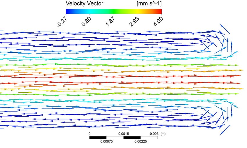
2 A. A. Dev, P. Dunne T. M. Hermans and B. Doudin
P1 L P2
a) b) Mag ne ts
III tf
II n Fe rro fluid
d D Antitube Curve d
I
Outle t
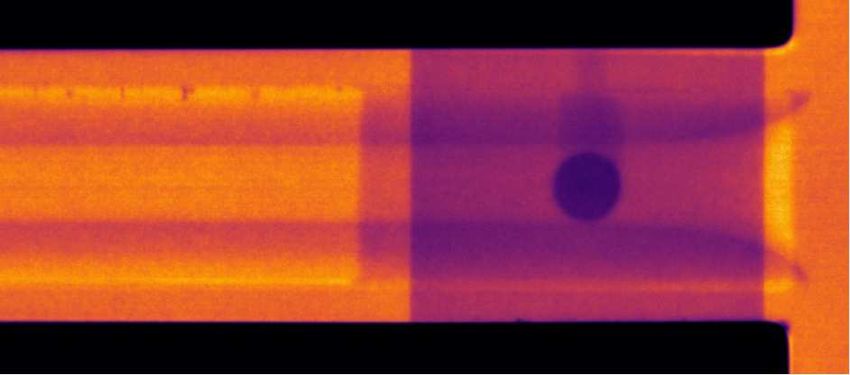
Figure 1. a) Experimental set up for differential pressure measurement (P1 , P2 ). An antitube
of diameter d inside a rigid cavity of diameter D is shown with a velocity profile following
the hypothesis of our 2-fluid, 3-region model. The red line between the ferrofluid and antitube
depicts the liquid-liquid interface. b) X-ray transmission image of the two-fluid system, inside a
cavity (D = 4.4 mm) surrounded by magnets. The brighter central flowing liquid (antitube) is
surrounded by a darker immiscible ferrofluid.
layer between the main turbulent flow and the solid walls promoting drag reduction
(Abubakar et al. 2014). In a laminar flow, the efficacy of an intermediate liquid layer
is limited due to the complications of injecting, stabilizing, and flowing two immiscible
liquids together. Such co-flowing liquid streams lack stable liquid-liquid interfaces during
shear flow (Hooper & Boyd 1983). Moreover, the injected flow tends to break up into
droplets, either immediately termed dripping, or along the flow under the action of
Rayleigh-Plateau instability (Utada et al. 2007).
Furthermore, for marine applications, drag-reduction liquids are considered to be inap-
propriate, as draining should be avoided, and the lubricating liquid should be of lower
viscosity than water to achieve a non-negligible drag reduction (Solomon et al. 2014;
Wexler et al. 2015). The use of ferrofluids as lubricating liquid can mitigate the first
issue, by using magnets to hold them in place. Recent results using ferrofluid-infused
surfaces indeed showed superhydrophobic behaviour of interest (Wang et al. 2018). The
possibility of drag reduction using magnetic fluids as lubricating liquids was pioneered
by Medvedev & Krakov (1983); Medvedev et al. (1987) and further studied by Krakov
et al. (1989) where they investigated how the pressure gradients can be reduced by
means of intermediate ferrofluids. We extend their considerations by clarifying how drag
reduction, defined as the percentage change in friction factor (Watanabe et al. 1999;
Fukuda et al. 2000; Karatay et al. 2013; Mirbod et al. 2017; Liu et al. 2020; Ayegba et al.
2020) is enhanced. Here we experimentally study the flow of viscous liquids separated
from the solid wall by an immiscible ferrofluid, under the condition that the lubricating
liquid does not escape as it is held in place by magnetic forces. Our experimental system
forms an ideal liquid in liquid tube system where the lubricating liquid forms a perfect
cylindrical encapsulation for the flowing liquid, using a magnetic force design best suited
to preserve the cylindrical geometry and providing optimum robustness of the system.
This makes possible comparisons of experiments with the simplest theories, as well as
check of the model for a significant range of hydrodynamic parameters. The study goes
beyond the assumption of unidirectional flow of the involved liquids (ideal for maximum
drag reduction) (Walsh et al. 2017; Solomon et al. 2014) and our approach drastically
reduces the pressure loss of the transported liquid, due to nearly frictionless flow.
2. Experiments
We investigate the flow properties of a diamagnetic cylindrical liquid magnetically con-
fined in a ferrofluid sheath (Dunne et al. 2020), termed an ’antitube’ (Coey et al. 2009).
The diamagnetic liquids are glycerol (Sigma Aldrich) and honey (Famille Michaud), and
the ferrofluids used are APG314 (F1) and APGE32 (F2) (FerroTech). Hence we have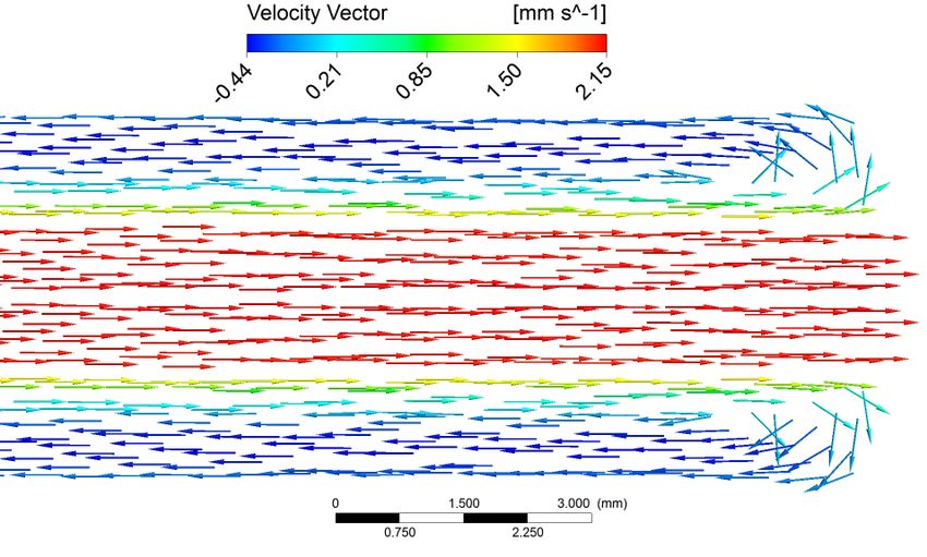
Fluid Drag Reduction by Magnetic Confinement                          3
four combinations of magnetic and non–magnetic liquids. The viscosities of these liquids
were measured using a viscometer (Anton Paar MCR 502); for glycerol it is constant
at 1.1 Pa.s and for honey 11.99 Pa.s under strain rate of 100 s−1 (maximum strain
rate in our experiments with honey in antitube is below 10 s−1 ). For ferrofluids see
SI S1. To perform the flow experiments, the four-magnet assembly was housed in a
3D-printed support as recently shown by Dunne et al. (2020) with additional built-in
fluidic connectors for pressure measurements (cross section Fig. 1a). The 3D printed
cavity (diameter D, Fig. 1a) is first filled with the non-magnetic liquid which is then
slowly replaced by injecting the ferrofluid into the cavity, resulting in the formation of
an antitube. We control the diameter of an antitube by varying the injected volume of
ferrofluid. Drag reduction was measured under flow, set by a syringe pump (Harvard
apparatus; PHD 2000), using the resulting pressure drop between the inlet and outlet of
the antitube measured by pressure sensors (Honeywell; HSCDLND001PG2A3). Fig. 1b)
shows an X-ray absorption image of the system. Near the ends of the magnets, the
antitube diameter increases due to the fringe magnetic fields. This results in curved
inlets and outlets for antitube channels (see SI S2) which will prove essential for trapping
the ferrofluid. Experiments were performed by flowing either honey or glycerol, confined
in either one of two commercial ferrofluids (F1, F2). This allowed measurements that
span a large viscosity ratio between transported and confining liquids, both larger and
smaller than one. Experiments were performed for three different antitube diameters.
For a fluid with density ρ, the measured pressure drop ∆P resulting from a flow rate Q
through a tube of diameter d and length L is related to the experimental friction factor
as (Karatay et al. 2013)

                                               π 2 ∆P d5
                                      fexp =                                            (2.1)
                                                8ρQ2 L
following which the drag reduction factor DR is defined as (Watanabe et al. 1999)

                                          fP − fexp
                                  DR =               × 100                             (2.2)
                                             fP
which is the percentage change of the measured friction factor fexp when compared to
the factor fP under the same flow rate that follows Poiseuille’s law fP = 16πDη/ρQ at a
solid wall boundary. We take D = 4.4 mm, the diameter of cavity in absence of encapsu-
lating ferrofluid (Fig. 1b). Due to the liquid-liquid interface, the zero-velocity boundary
condition at the transported liquid wall (antitube–ferrofluid interface) is not valid, and
the deviation from Poiseuille’s law should result in hydrodynamic drag reduction.
Experiments performed for four different viscosity ratios (ηr ); Honey-F1 with viscosity
ratio ηr = 52 (Fig. 2a), Honey-F2 with viscosity ratio ηr = 7 (Fig. 2b), Glycerol-F1
with viscosity ratio ηr = 4.8 (Fig. 2c) and Glycerol-F2 with viscosity ratio ηr = 0.65
(Fig. 2d) show remarkably high drag reductions ranging from 80 % to 99.8 %. It can be
seen that with increase in viscosity ratio, drag reduction increases. In contrast to prior
expectations (Solomon et al. 2014), large drag reduction can still be achieved, even if
the encapsulating/lubricating ferrofluid has a higher viscosity than the transported one,
such as for Glycerol-F2, where a drag reduction of up to 95% is observed (Fig. 2d).
As one would expect, the drag reduction increases with decreasing antitube diameter
(Fig. 2a,b,c,d).
The large drag reduction can also be expressed as a much reduced pressure drop in the
liquid-in-liquid design, ∆Pexp , compared to a solid-wall interface, ∆PP , of equivalent size
(diameter d) with an improvement ratio αp = ∆PP /∆Pexp . Fig. 3 shows that αp of more
4 A. A. Dev, P. Dunne T. M. Hermans and B. Doudin
Honey-F2 (ηr= 7.0)
a) 100
Honey-F1 (ηr= 52)
2.45
b) 100 2.40
1.77 1.85
99 0.98 98 1.20
DR (%)
DR (%)
96
98
94
97 Line s : Analytical
92
Marke rs : Nume rical
Fille d marke rs : Expe rime ntal
96 90
0 0.5 1 0 0.5 1
Q (ml/min) Q (ml/min)
Glycerol-F1 (ηr= 4.8) Glycerol-F2 (ηr = 0.65)
c) 100 2.30
d) 100 2.30
1.72 1.53
95 1.07 1.05
DR (%)
90
DR (%)
90
85 80
Line s : Analytical
Marke rs : Nume rical
80 Fille d marke rs : Expe rime ntal
70
75
0 0.5 1 1.5 0 0.5 1 1.5
Q (ml/min) Q (ml/min)
Figure 2. Drag reduction, DR, for three antitube diameters as a function of flow rate is plotted
for a) honey as the transported liquid with APG314 ferrofluid (F1) as the confining liquid, b)
honey with APGE32 ferrofluid (F2), c) glycerol with F1 and d) glycerol with F2. ηr is the ratio
between the antitube and ferrofluid viscosities. Legend shows the antitube diameter in mm.
Lines, markers and filled markers compare theory, numerics and experiments.
than two orders of magnitude can be achieved. For ηr =52, the antitube system results
in 157 times less pressure drop than the solid walled tube (red markers in Fig. 3a)).
Interestingly for viscosity ratio ηr =0.65 results in almost 6 times smaller pressure drop
(red markers in Fig. 3d)). As expected the improvement ratio αp increases with decrease
in diameter of antitube (Fig. 3a,b,c,d).
3. Modelling
We explain our results using a two-fluid three-region model, based on the steady-state
one dimensional Navier-Stokes equation with velocity as a function of radius only in a
cylindrical geometry, u = u(r), with modified boundary conditions. A key hypothesis is
the occurrence of a counter flow within the encapsulating ferrofluid (Fig. 1a) resulting
from avoiding drainage of the ferrofluid by using magnetic sources. This suppression is due
to the non-uniform magnetic fields at the inlet and outlet opposing any egress of ferrofluid.
As the ferrofluid cannot escape, but noting that i) flux must be conserved and ii) that the
drag reduction should result from a non-zero velocity at the ferrofluid-antitube interface,
a return path for the ferrofluid flow must exist. The simplest hypothesis is illustrated by
the velocity profile in Fig. 1a, where we define three regions: I inside the antitube, II the
part of the ferrofluid that travels alongside the antitube flow, and III where counter-flow
occurs. The non-dimensional governing equations for the three regions (i = I, II, II) are
given byFluid Drag Reduction by Magnetic Confinement 5
Honey-F1 (ηr= 52) Honey-F2 (ηr= 7.0)
a) 2.45 b)20 2.40
150 1.77 1.85
0.98 1.20
15
100
50 10
0 5
0 0.5 1 0 0.5 1
Q (ml/min) Q (ml/min)
Glycerol-F1 (ηr= 4.8) Glycerol-F2 (ηr= 0.65)
c) 20 d) 6 2.30
2.30 1.53
1.72 1.05
1.07
15 4
10 2
5 0
0 0.5 1 1.5 0 0.5 1 1.5
Q (ml/min) Q (ml/min)
Figure 3. Pressure drop reduction. a) Honey-APG314 (ηr =52), b) Honey-APGE32 (ηr =7.0), c)
∆Pp
Glycerol-APG314 (ηr =4.8), d) Glycerol-APGE32 (ηr =0.65). αp = ∆Pexp is the ratio of pressure
drop for solid wall tube to the antitube with identical diameter. The error bars are smaller than
the size of markers where not visible.
?
∂Pi?
1 ∂ ? ∂ui
? ?
r ?
= (3.1)
Rei r ∂r ∂r ∂z ?
where u?i ,r? ,z ? are dimensionless velocity and coordinates scaled by the average velocity
u0 of the flowing liquid and diameter d of the region I (antitube). The dimensionless
pressure is defined as Pi? = Pi /ρi u20 with the corresponding Reynolds numbers for each
region being Rei = ρi u0 d/ηi . Note that the pressure gradients along the main flow in
both ferrofluid regions are equal, under the hypothesis that these two regions do not mix,
∂P ? ?
∂PIII
resulting in the absence of pressure gradient along r, and therefore ∂zII ? = ∂z ? . Since
the magnetic-nonmagnetic interface is modelled as a non-deforming fixed liquid wall of
infinitesimal thickness, the pressure gradients in region I and II are assumed different.
This hypothesis allows us to consider a diameter d, set experimentally by the amount of
ferrofluid trapped in the cavity, independent of the flow rate. Deviations are only expected
at the tube extremities, over a length that we neglect when compared to the device
length. These governing equations are solved for all velocities (u?I , u?II , u?III ), the pressure
∂P ?
gradient ∂zIII ? and the thickness n of region II, using boundary conditions depicted in
the Fig. 1a): finite velocity at the antitube centre, zero velocity at the solid wall and at
interface of II and III, continuity of velocity and shear stress at interfaces I-II and II-III.
Along with these boundary conditions, the volume conservation of ferrofluid dictates that
Q?II = −Q?III . We present two models, one with no assumption (full model) and another6 A. A. Dev, P. Dunne T. M. Hermans and B. Doudin
∂P ?
with assumption ∂zII
? = 0, which explicitly shows the contribution of geometric and fluid
parameters for drag reduction.
3.1. Full model
In the full model Eq. 3.1 expands to
∂u? ?
∂
1 ∂PIII
r? III = (3.2)
ReIII r ∂r?
? ∂r? ∂z ?
? ?
1
? ∂uII∂ ∂PII
r = (3.3)
ReII r? ∂r?
∂r? ∂z ?
?
∂PI?
1 ∂ ? ∂uI
r = (3.4)
ReI r? ∂r? ∂r? ∂z ?
Solving which with the boundary conditions mentioned above in text gives the analytical
expressions of the velocity profiles as:
? h 2
ReIII ∂PIII i
u?III = r ?
− a1 ln(r ?
) − a2 (3.5)
4 ∂z ?
" 2 ! #
?
ρI ∂PI? ?
2dr?
ReII ∂PIII ?2 d + 2n 1 ∂PIII
u?II = r − + − ln
4 ∂z ? 2d 2 ρII ∂z ? ∂z ? d + 2n
(3.6)
ReI ∂PI? h ?2 i
u?I = r + 4(a3 − a4 − a 5 ) (3.7)
4 ∂z ?
where, a1 ,a2 , a3 ,a4 ,a5 are scalar constants that can be expressed as explicit functions of
d, and the thicknesses n of the region II and tf of the ferrofluid. These constants required
in velocity profiles are
(d + 2tf )2 − (d + 2n)2
1
a1 = (3.8)
4d2 d+2tf
ln d+2n
d+2tf
(d + 2tf ) 2 ln 2d
2
(d + 2n) − (d + 2tf ) 2
a2 = + (3.9)
4d2 d+2t
ln d+2nf 4d2
" 2 #
1 d + 2n 1 1 d + 2n 1 1 1
a3 = ηr − , a4 = ln ηr + , a5 = (3.10)
32a6 2d 4 4 d 2 16a6 16
Since the diameter of antitube (d) increases near the edge of magnet, we use the weighted
average of the diameter along the length and get an average constant diameter as
14
1 i=L/l
L4 X l
= 4
(3.11)
d i=1
di
where, l is the small length over which the diameter is considered constant. We consider
l equals 0.1 mm and L= 51 mm. Note n is unknown and to find that we use the
experimental diameter of antitube d, thickness of ferrofluid tf in the condition of volumeFluid Drag Reduction by Magnetic Confinement 7
conservation of ferrofluid Q?II = −Q?III and continuity of shear stress at the interface II
and III, given by
?
∂PIII 1 ρI ∂PI?
= − (3.12)
∂z ? 8a6 ρII ∂z ?
?
∂PIII 2a8 ρI ∂PI?
?
=− (3.13)
∂z a7 − 2a8 + a9 ρII ∂z ?
The artefact of different pressure gradients in Eq. 3.12 and Eq. 3.13 results from our
simplified hypothesis considering liquid-liquid interface as a non-deformable fixed liquid
wall. This avoids solving a pressure equation including magnetic stress which would
further complicate the model and would result in a non-linear governing equation.
Using Eq. 3.12 and Eq. 3.13, we can write
1 2a8
= (3.14)
8a6 a7 − 2a8 + a9
n can be analytically calculated using Eq. 3.14 because the parameters a6 ,a7 ,a8 ,a9 are
functions of n,d and tf where d and tf are known and fixed by experiments. Where a6
to a9 as
" 2 2 !#
1 d + 2n 1 1 d + 2n a1
a6 = − − 2− (3.15)
2 2d 8 4 2d d+2n 2
2d
(d + 2n)4 (d + 2n)2
1
a7 = − − + (3.16)
64d4 64 32d2
(d + 2n)2
1 1 1 1 1 d + 2n
a8 = − − ln + + ln (3.17)
4 16d2 8 2 16 8 2d
(d + 2tf )4 (d + 2n)4 d + 2tf (d + 2tf )2 (d + 2tf )2
a9 = 4
− 4
− a 1 ln 2
−
64d 64d 2d 8d 16d2
(3.18)
d + 2n (d + 2n)2 (d + 2n)2 (d + 2tf )2 (d + 2n)2
− ln − − a2 −
2d 8d2 16d2 8d2 8d2
The flow rate through antitube is obtained by integrating Eq. 3.7 over the cross section
area of antitube and is given by
πReI ∂PI? 1
Q?I = + a3 − a4 − a5 (3.19)
4 ∂z ? 32
∂PI? −fA
Noting here that ∂z ? = 2 , where fA is the friction factor and using Eq. 3.19 results
in
fA = 64/ReI β (3.20)
where
β = 32(a5 + a4 − a3 ) − 1 (3.21)
3.2. Simplified model (Assuming pure shear driven flow in region II)
The full model is fully analytically solvable, however Eq. 3.20 and Eq. 3.21 together
presents a complex expression where the contribution of fluid and geometric properties
are hidden. To explicitly show the contribution of fluid and geometric properties towards
drag reduction, we neglect the pressure gradient in region II. After neglecting the pressure8 A. A. Dev, P. Dunne T. M. Hermans and B. Doudin
gradient in region II (in Eq. 3.3), and solving the governing equations with the boundary
conditions as used in the full model gives velocity profiles in three regions as
? h 2
ReIII ∂PIII i
u?III = ?
r? − a1 ln(r? ) − a2 (3.22)
4 ∂z
ηr ∂PI? 2dr?
u?II = ReI ln (3.23)
8 ∂z ? d + 2n0
" 2 #
∂PI? r?
ηr d 1
?
uI = ReI ? + ln − (3.24)
∂z 4 8 d + 2n0 16
n0 is again calculated using expressions resulting from condition of volume conservation
of ferrofluid and shear stress continuity at the interface between region II and III. The
flow rate through the antitube is obtained by integrating Eq. 3.24 and is given by
πReI ∂PI? 1
d 1
Q?I = ln ηr − (3.25)
4 ∂z ? 8 d + 2n0 32
And the friction factor is fA = 64/ReI β0 , where
2n0
β0 = 1 + 4 ln 1 + ηr (3.26)
d
4. Numerical visualisation of counter flow
Detailed information on the occurrence of counter flow and the resulting velocity vector
field is obtained by computational fluid dynamics (CFD) simulations using ANSYS CFX
18. In the numerical simulations, we solve the three-dimensional Navier–Stokes equation
by considering the magnetic-nonmagnetic interface as a non-deformable fixed liquid wall
of infinitesimal thickness. The axial velocity and shear stress are equal on both sides of
the wall (continuous across the interface). Since the magnetic field gradient only exists
in the radial direction far from the inlet or outlet, no magnetic body force is considered
on the ferrofluid. The finite curved edges of ferrofluid near inlet and exit of the flow is
modelled as a free slip wall with zero normal velocity (no flow across the curved edges)
(See SI S3 for numerical algorithm). As illustrated in Fig. 4, a counter flow behaviour
occurs in the ferrofluid close to the outer wall for Honey-F1 with d = 1.73 mm (Fig. 4a)
and Glycerol-F2 with d = 1.54 mm (Fig. 4b). Flow rate is fixed at Q = 300 µl min−1 .
A similar velocity profile with counter flow in the ferrrofluid is also presented by Krakov
et al. (1989) as a solution of their two fluid model. Furthermore, good agreement between
numerical and analytical velocity profiles using the full model for both Honey-F1, ηr =52
(Fig. 4c), and Glycerol-F2, ηr =0.65, (Fig. 4d) validates our numerical algorithm. The
simplified model obtained by neglecting pressure gradient term is also compared with
the numerical calculations shown in Fig. 4e and Fig. 4f. The difference between the
two analytical models is apparent on comparing Fig. 4c with Fig. 4e and Fig. 4d with
Fig. 4f. In order to more accurately model the experimental system shown in Fig. 1, we
extended the simulations to consider the finite length of a device, and the effect of fringe
fields on the shape of interface at the inlet and outlet (curved inlet and outlet, Fig. 1b),
beyond the hypothesis of the infinite tube of the analytical model. Numerical simulations
were found to reproduce well the drag reduction data in Fig. 2a) , while systematically
underestimating observed drag reduction for ηr = 0.65 (Fig. 2d). Note that the numerical
drag reduction is calculated using Eq. 2.1 and Eq. 2.2 with ∆P obtained numerically.Fluid Drag Reduction by Magnetic Confinement 9
-0.44 0.21 0.85 1.50 2.15 Velocity -0.27 0.80 1.87 2.93 4.0
[mm s-1]
a) b)
3 mm
Honey-F1 (ηr= 52) Glycerol-F2 (ηr= 0.65)
c) 1 d) 1
0.5 0.5
0.5
0
0 -0.5
0
0.99 1 1.01
-0.5 -0.5
-1 -1
0 0.5 1 0 0.5 1 1.5
e) 1 f)
1
0.5 0.5
0.5
0
0 -0.5 0
0.99 1 1.01
-0.5 -0.5
-1 -1
0 0.5 1 0 0.5 1 1.5
Figure 4. Numerical visualization of counter flow. a) and b) Velocity vectors near the
outlet showing reverse flow for Honey-F1 and Glycerol-F2 respectively. c) and d) comparison
of analytical and numerical non dimensional velocity profile in Fig. 4(a) and Fig. 4(b) using
full model. e) and f) comparison using simplified analytical model neglecting pressure gradient
term. Lines are analytical predictions and markers are numerical calculations. Inset shows the
magnified view of velocity profile in antitube. The antitube diameter for left and right column
is 1.73 mm and 1.54 mm respectively. ηr is viscosity ratio.
5. Discussion
The simple analytical model captures the experimental measurements for the four liquid
combinations, spanning four orders of magnitude of the modified Reynolds number.
Fig. 5 illustrates how the calculated friction factor fA (from Eq. 3.20 and Eq. 3.21)
compares with the experimental one fexp (computed using Eq. 2.1). The friction factor
fA is similar to the fit parameter presented by Krakov et al. (1989). We provide here
full analytical expressions for fA , necessary for the equation of the drag reduction
defined as percentage change in friction factor fA with respect to friction factor for
Poiseuille flow fP . Similar reduction of friction factor (Eq. 3.20) by an additional
factor (here β, Eq. 3.21) is also shown by Watanabe et al. (1999) for a highly water-
repellent wall system. Note that all the experimental data from Fig. 2 are presented
in Fig. 5. Although the model cannot completely account for minor offsets observed at
low viscosity ratio values, Fig. 5 nevertheless illustrates the significant range of fluidic
conditions that the model can apply to. Note that a significant variation of drag reduction10 A. A. Dev, P. Dunne T. M. Hermans and B. Doudin
10 5
Honey
F1 F2
2.45 2.40
1.77 1.85
0.98 1.20
10 4
fA and fexp
10 3
Glycerol
F1 F2
2.30 2.30
1.72 1.53
1.07 1.05
10 2
10 -3 10 -2 10 -1 10 0
Re β
Figure 5. Comparison of experimental fexp (markers) and analytical fA (line) friction factors.
Inset gives the diameter of antitubes (mm) for each case. Re denotes the Reynolds number and
β is the scaling factor (= 1 for solid-walled tube).
Case d (mm) tf (mm) n (mm) β n0 (mm) β0
2.45 0.98 0.34 41.6 0.38 58.68
Honey-APG314 1.77 1.32 0.49 74 0.53 98.3
0.98 1.71 0.67 151.68 0.73 183.35
2.40 1.00 0.36 6.74 0.39 9.12
Honey-APGE32 1.85 1.28 0.47 10.21 0.51 13.39
1.20 1.60 0.61 17.44 0.67 21.49
2.30 1.05 0.38 5.24 0.41 6.95
Glycerol-APG314 1.72 1.34 0.50 7.98 0.54 10.26
1.07 1.67 0.65 13.62 0.70 16.46
2.3 1.05 0.38 1.57 0.41 1.8
Glycerol-APGE32 1.53 1.44 0.54 2.11 0.58 2.44
1.05 1.68 0.65 2.74 0.71 3.12
Table 1. Comparison of the full and simplified models
with flow rate is found for the largest viscosity ratio (ηr = 52). In such cases, the
pressure drop becomes very small at small flow rates, and the experimental difficulties
in neglecting the pressure loss related to the interconnects and pressure indicators limit
the reliability of the data, systematically underestimating the drag reduction values. We
expect that more complicated fluid velocity profiles along z can develop, especially for
high viscosity encapsulating liquids where the magnetic/non-magnetic interface might
deform significantly due to high pressure drop, but taking them into account is beyond
our current model.Fluid Drag Reduction by Magnetic Confinement 11
?
∂PII
A simplified expression for β that suppose pure shear driven flow in region II ( ∂z ? =0)
is given by Eq. 5.1.
2n0
β0 = 1 + 4 ln 1 + ηr (5.1)
d
β0 expresses the deviation from the asymptotic β0 = 1 value for solid walls, and quantifies
the reduction in the friction resulting from a liquid-in-liquid flow. This scaling number
β0 controls the drag reduction magnitude through the viscosity ratio ηr of the involved
liquids, the size of antitube (d), and thickness of the ferrofluid region tf (typically n0 ≈ 0.4
tf ). Note that we take the viscosity of the ferrofluid at saturation in a magnetic field (see
SI S1). Hence this approximation of β underestimates the frictional drag (also apparent
in numerical results, Fig. 4) and becomes more apparent when the thickness of the
ferrofluid decreases (see Table 1). It, however, explicitly reveals the contributions of the
antitube geometry and fluid properties. The drag reduction can be tuned by the choice
of viscosities and the amount of ferrofluid trapped in the device cavity.
6. Conclusions
We have studied the flow of viscous liquids through cylindrical liquid-in-liquid tube
where the encapsulating liquid is held in place by a quadrupolar magnetic field. Our
results indicate that spectacularly large drag reductions (up to 99.8%) can be achieved
by taking advantage of the non-zero velocity of a viscous liquid at its interface with the
encapsulating liquid. The friction reduction is quantified by rescaling of the Reynolds
number with scaling factor β in Eq. 3.21.
The drag reduction impoves when decreasing the diameter of an antitube relative to
its surrounding ferrofluid, or when increasing the ratio of the antitube to ferrofluid
viscosities. The former is relevant for the needs and length-scales of microfluidics,
while the latter indicates that large drag reduction is expected when flowing highly
viscous antitube liquids. Moreover, with antitube diameters as small as 10 µm already
achievable(Dunne et al. 2020), antitube diameter to ferrofluid thickness ratios of order
100 are within reach. Therefore very large drag reduction in microfluidic channels is
possible for a broad range of encapsulating liquid viscosities. Downsizing or designing
magnetic force gradients along the flow direction can also further enhance the stability
of the ferrofluid against shearing, paving the way to both high velocity and low viscosity
fluidic applications in domains ranging from nanofluidics to marine or hydrocarbon
cargo transport.
Acknowledgements. This project has received funding from the European Union’s
Horizon 2020 research and innovation programme under the Marie Skłodowska-Curie
grant agreement No 766007. We also acknowledge the support of the University of
Strasbourg Institute for Advanced Studies (USIAS) Fellowship, and French National
Research Agency (ANR) through the Programme d’Investissement d’Avenir under
contract ANR-11-LABX-0058-NIE within the Investissement d’Avenir program ANR-
10-IDEX-0002-02. We thank A. Zaben, Prof. Cēbers and Dr. Kitenbergs of MMML lab,
Riga, Latvia for ANSYS CFD software facility and magnetoviscosity measurements.
Declaration of interests. The authors report no conflict of interest.12 A. A. Dev, P. Dunne T. M. Hermans and B. Doudin
REFERENCES
Abubakar, A., Al-Wahaibi, T., Al-Wahaibi, Y., Al-Hashmi, A.R. & Al-Ajmi, A. 2014
Roles of drag reducing polymers in single- and multi-phase flows. Chemical Engineering
Research and Design 92 (11), 2153–2181.
Atencia, Javier & Beebe, David 2005 Controlled microfluidic interfaces. Nature 437, 648–55.
Ayegba, Paul O., Edomwonyi-Otu, Lawrence C., Yusuf, Nurudeen & Abubakar,
Abdulkareem 2020 A review of drag reduction by additives in curved pipes for single-
phase liquid and two-phase flows. Engineering Reports p. e12294.
Brostow, W. 2008 Drag reduction in flow: Review of applications, mechanism and prediction.
Journal of Industrial and Engineering Chemistry 14 (4), 409 – 416.
Choi, C-H. & Kim, C-J. 2006 Large slip of aqueous liquid flow over a nanoengineered
superhydrophobic surface. Phys. Rev. Lett. 96, 066001.
Coey, J. Michael D., Aogaki, Ryoichi, Byrne, Fiona & Stamenov, Plamen
2009 Magnetic stabilization and vorticity in submillimeter paramagnetic liquid tubes.
Proceedings of the National Academy of Sciences 106 (22), 8811–8817.
Dunne, P., Adachi, T., Dev, A. A., Sorrenti, A., Giacchetti, L., Bonnin, A.,
Bourdon, C., Mangin, P. H., Coey, J. M. D., Doudin, B. & Hermans, T. M.
2020 Liquid flow and control without solid walls. Nature 581, 58–62.
Ensikat, H.J., Ditsche-Kuru, P., Neinhuis, C. & Barthlott, W. 2011 Superhydropho-
bicity in perfection: the outstanding properties of the lotus leaf. Beilstein Journal of
Nanotechnology 2, 152–161.
Fukuda, Kazuhiro, Tokunaga, Junichiro, Nobunaga, Takashi, Nakatani, Tatsuo,
Iwasaki, Toru & Kunitake, Yoshikuni 2000 Frictional drag reduction with air
lubricant over a super-water repellent surface. Journal of Marine Science and Technology
5, 123–130.
Grein, T. A., Loewe, D., Dieken, H., Weidner, T., Salzig, D. & Czermak, P. 2019
Aeration and shear stress are critical process parameters for the production of oncolytic
measles virus. Frontiers in Bioengineering and Biotechnology 7, 78.
Holmberg, K. & Erdemir, A. 2017 Influence of tribology on global energy consumption,
costs and emissions. Friction 05 (03), 263.
Hooper, A. P. & Boyd, W. G. C. 1983 Shear-flow instability at the interface between two
viscous fluids. Journal of Fluid Mechanics 128, 507–528.
Hu, H., Wen, J., Bao, L., Jia, L., Song, D., Song, B., Pan, G., Scaraggi, M., Dini, D.,
Xue, Q. & Zhou, F. 2017 Significant and stable drag reduction with air rings confined
by alternated superhydrophobic and hydrophilic strips. Science Advances 3 (9).
Karatay, E., Haase, A. S., Visser, C. W., Sun, C., Lohse, D., Tsai, P. A. &
Lammertink, Rob G. H. 2013 Control of slippage with tunable bubble mattresses.
Proceedings of the National Academy of Sciences 110 (21), 8422–8426.
Krakov, M. S., Maskalik, E. S. & Medvedev, V. F. 1989 Hydrodynamic resistance of
pipelines with a magnetic fluid coating. Fluid Dynamics 24 (5), 715–720.
Lee, S. & Spencer, N. D. 2008 Sweet, hairy, soft, and slippery. Science 319 (5863), 575–576.
Liu, Weili, Ni, Hongjian, Wang, Peng & Zhou, Yi 2020 An investigation on the drag
reduction performance of bioinspired pipeline surfaces with transverse microgrooves.
Beilstein Journal of Nanotechnology 11, 24–40.
Medvedev, V.F. & Krakov, M.S. 1983 Flow separation control by means of magnetic fluid.
Journal of Magnetism and Magnetic Materials 39 (1), 119 – 122.
Medvedev, V.F., Krakov, M.S., Mascalik, E.S. & Nikiforov, I.V. 1987 Reducing
resistance by means of magnetic fluid. Journal of Magnetism and Magnetic Materials
65 (2), 339 – 342.
Mirbod, Parisa, Wu, Zhenxing & Ahmadi, Goodarz 2017 Laminar flow drag reduction
on soft porous media. Scientific Reports 7.
Mitchell, M. J. & King, M. R. 2013 Computational and experimental models of cancer cell
response to fluid shear stress. Frontiers in Oncology 3, 44.
Nesyn, G., Manzhai, V., Suleimanova, Yu, Stankevich, V. & Konovalov, K. 2012
Polymer drag-reducing agents for transportation of hydrocarbon liquids: Mechanism of
action, estimation of efficiency, and features of production. Polymer Science Series A 54.
Reinke, W., Gaehtgens, P. & Johnson, P. C. 1987 Blood viscosity in small tubes: effectFluid Drag Reduction by Magnetic Confinement 13
of shear rate, aggregation, and sedimentation. American Journal of Physiology-Heart and
Circulatory Physiology 253 (3), H540–H547.
Saranadhi, Dhananjai, Chen, Dayong, Kleingartner, Justin A., Srinivasan,
Siddarth, Cohen, Robert E. & McKinley, Gareth H. 2016 Sustained drag
reduction in a turbulent flow using a low-temperature leidenfrost surface. Science Advances
2 (10).
Sayfidinov, K., Cezan, S. Doruk, Baytekin, B. & Baytekin, H. Tarik 2018 Minimizing
friction, wear, and energy losses by eliminating contact charging. Science Advances 4 (11).
Solomon, B., Khalil, K. & Varanasi, K. 2014 Drag reduction using lubricant-impregnated
surfaces in viscous laminar flow. Langmuir : the ACS journal of surfaces and colloids 30.
Utada, Andrew S., Fernandez-Nieves, Alberto, Stone, Howard A. & Weitz,
David A. 2007 Dripping to jetting transitions in coflowing liquid streams. Phys. Rev.
Lett. 99, 094502.
Walsh, Edmond, Feuerborn, Alexander, Wheeler, James, Tan, Ann, Durham,
William, Foster, Kevin & Cook, Peter 2017 Microfluidics with fluid walls. Nature
Communications 8.
Wang, W., Timonen, J., Carlson, A., Drotlef, D-M., Zhang, C., Kolle, S.,
Grinthal, A., Wong, T. S., Hatton, B., Kang, S., Kennedy, S., Chi, J., Blough,
R., Sitti, M., Mahadevan, L. & Aizenberg, J. 2018 Multifunctional ferrofluid-infused
surfaces with reconfigurable multiscale topography. Nature 559, 77–82.
Watanabe, K., Udagawa, Y. & Udagawa, H. 1999 Drag reduction of newtonian fluid in a
circular pipe with a highly water-repellent wall. Journal of Fluid Mechanics 381, 225–238.
Wexler, Jason S., Jacobi, Ian & Stone, Howard A. 2015 Shear-driven failure of liquid-
infused surfaces. Phys. Rev. Lett. 114, 168301.
Wong, T-S., Kang, S. H., Tang, K. Y. S., Smythe, E. J., Hatton, B. D., Grinthal, A.
& Aizenberg, J. 2011 Bioinspired self-repairing slippery surfaces with pressure-stable
omniphobicity. Nature 477, 443–447.You can also read