Supplement of Intercomparison of MAX-DOAS vertical profile retrieval algorithms: stud- ies on field data from the CINDI-2 campaign
←
→
Page content transcription
If your browser does not render page correctly, please read the page content below
Supplement of Atmos. Meas. Tech., 14, 1–35, 2021
https://doi.org/10.5194/amt-14-1-2021-supplement
© Author(s) 2021. This work is distributed under
the Creative Commons Attribution 4.0 License.

Supplement of
Intercomparison of MAX-DOAS vertical profile retrieval algorithms: stud-
ies on field data from the CINDI-2 campaign
Jan-Lukas Tirpitz et al.

Correspondence to: Jan-Lukas Tirpitz (jan-lukas.tirpitz@iup.uni-heidelberg.de)

The copyright of individual parts of the supplement might differ from the CC BY 4.0 License.
S1   M3 algorithm description

     The M3 algorithm developed at the Ludwig-Maximilians-University in Munich is an OEM algorithm with Newton Gauss
     optimization. The radiative transfer model LibRadTran (Mayer and Kylling, 2005) serves as forward model for the retrieval.
     LibRadTran provides several radiative transfer equation solvers which can handle both pseudo spherical and full spherical
5    geometry. The Jacobian is calculated numerically using the finite difference method, while the box air mass factors for trace gas
     profile retrievals are calculated using the Monte Carlo module of LibRadTran (MYSTIC). The M3 retrieval used in the CINDI-
     2 campaign is a modified version of the algorithm described in detail in Chan et al. (2019) with the iterative optimization of
     the a priori profile disabled. Aerosol extinction profiles are retrieved in the linear space.

     S2   O4 scaling factor

10   By some groups, the O4 scaling factor SF is applied to the measured dSCDs before the profile inversion. Initial motivation
     for its application are previous MAX-DOAS retrieval studies (e.g Wagner et al., 2009; Clémer et al., 2010) which report on
     a significant mismatch between measured and simulated dSCDs and/ or between MAX-DOAS integrated aerosol extinction
     and simultaneously measured sun photometer AOT that could not yet be explained (Wagner et al., 2019; Ortega et al., 2016).
     Meanwhile a series of studies use an SF , empirically determined to values between 0.75 and 0.9.
15      As described in Sect. 2.1.3, in this study no scaling of O4 measured dSCDs was applied, except for MPIC-mp0.8 (MAPA
     algorithm with SF = 0.8). For CINDI-2, a SF of 0.8 was observed to enhance the number of valid profiles retrieved by
     MAPA and to significantly improve the agreement to the sun photometer total AOT in particularly in the UV (Beirle et al.
     (2019) and within this study). However, as mentioned before, for MAPA (as a parametrized approach without a priori profile
     and AVKs), a PAC as described in Sect. 3.4, cannot be correctly applied and thus deviations to the sun photometer are expected.
20   To further investigate the impact and necessity of the SF for CINDI-2 retrievals, also HEIPRO (as an OEM retrieval) was run
     with different SF s. In Fig. S1 the impacts of the SF and the PAC on the agreement between MAX-DOAS profiling results
     (of HEIPRO and MAPA) and the sun photometer are directly compared. Application of SF = 0.8 or the PAC, respectively,
     lead to a very similar improvement in the agreement (regarding RMS), while the application of both together results in a clear
     overcompensation. This suggests that the PAC and SF = 0.8 are equivalent to a large extent and that in the case of MAPA the
25   SF is a way to at least partly account for high-altitude aerosol when it comes to retrieving total AOTs. On the other hand a
     closer look reveals that if only the PAC is applied, a systematic negative offset of ≈ −0.04 remains in the correlation (for both
     algorithms and also other participants, compare to main text Sect. 3.4). Indeed, the top row of Fig. S3 shows that for HEIPRO
     the best RMSD is observed for SF = 0.92 ± 0.02 (UV). Regarding Aerosol Vis (Figure S2), the impact of high aerosol is
     smaller due to the enhanced vertical sensitivity range (see AVKs in main text Sect. 3.1), such that applying the same scaling
30   factor SF = 0.8 as for the UV (without PAC) should already lead to an overcompensation. Indeed, this is observed for HEIPRO
     as well as MAPA. The bottom row of Fig. S3 shows that, in contrast to the UV spectral range, the best agreement between sun
     photometer and MAX-DOAS in the Vis is observed for an SF > 1.
        The second indicator for the need of a scaling factor is a significant mismatch between modelled and measured dSCDs.
     Figure S4 shows, that for HEIPRO the application of an SF < 1 indeed improves the agreement between measured and
35   modelled O4 UV dSCDs by up to 35 % in RMSD under clear-sky conditions. Modelled dSCDs are systematically lower than
     the measured dSCDs in particular for higher elevation angles. Also, Wagner et al. (2009) reported that, under low aerosol
     conditions, measured dSCDs sometimes even significantly exceed dSCDs modelled within an aerosol free atmosphere, where
     O4 dSCDs are close to the largest possible (regarding clear-sky scenarios only). Therefore, the median measured dSCDs
     during CINDI-2 at low aerosol load (τs < 0.1) were compared to a set of aerosol free modelled dSCDs, showing that this did
40   not happen during CINDI-2 except for the two highest elevation angles α = 15◦ and 30◦ .
        Finally, as already stated by Beirle et al. (2019) applying SF = 0.8 to MAPA leads to an increased number of valid profiles
     (see Sect. S3), which again indicates that scaling brings the RTM closer to reality.
        The conclusions drawn are as follows: Even without O4 dSCD scaling, reasonable results and agreement with supporting
     observations are achieved (if a PAC is applied). In general, a scaling factor of 0.8 seems to be too small but might at least
45   partly be used to account for high-altitude aerosol for algorithms, that cannot quantify their sensitivity or the assimilated a

                                                                    1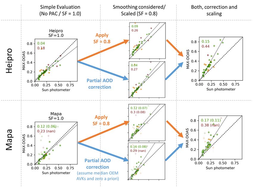
priori information. However, there are indications that a less extreme scaling (0.8 < SF < 1.0) might in general improve the
retrieval. Finally, we think that for this study the prescribed SF = 1.0 is justified. Even though it might not be ideal, it is the
most straightforward approach and yields reasonable and consistent results within the uncertainties introduced by other factors.
To draw more concise conclusions, further studies similar to Wagner et al. (2019) are necessary.

Figure S1. The impact of SF = 0.8 and PAC on the agreement between sun photometer and MAX-DOAS AOT (Aerosol UV) in the case
of HEIPRO (OEM approach, top row) and MAPA (parametrized approach, bottom row) in a direct comparison. Axes limits and labels of
the plots on the left apply for all plots in the figure. Left column: A standard retrieval with SF = 1 yields a clear underestimation of the sun
photometer AOT for both algorithms. Middle column: Applying the PAC or SF = 0.8 leads to a significant improvement. Right column:
Applying both leads to overcompensation. Note, that the PAC for MAPA incorporates vague assumptions (median AVKs from all OEM
algorithms and xa = 0) and is therefore less meaningful.

                                                                       2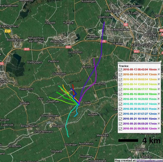
Figure S2. The impact of SF and PAC on Aerosol Vis results. Description of Fig. S1 applies. Due to the extended vertical sensitivity range of
the MAX-DOAS observations (compare to main text Sect. 3.1), the effect of high-altitude aerosol is less significant. While this is accounted
for in the PAC, the application of the same SF = 0.8 as for Aerosol UV leads to an overcompensation here already without additionally
applying the PAC.

                                                                     3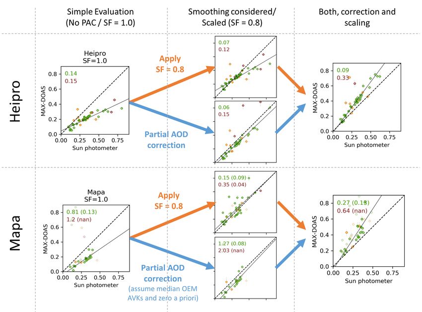
Figure S3. Correlation between the sun photometer AOT (PAC applied) and the HEIPRO algorithms for different SF for Aerosol UV (top
row) and Aerosol Vis (bottom row). Symbol colours differentiate between clear-sky (green), and cloudy conditions (orange, red). Numbers
in the upper left corners show the corresponding RMSD values. Interestingly, the best agreement for the two spectral ranges is found for
different scaling factors, namely for SF = 0.92 ± 0.02 (UV) and SF > 1 ± 0.02 (Vis). The thin line depicts the linear fit for clear-sky data
only.

Figure S4. Agreement between modelled and measured dSCDs (depicted as histograms of the ratio) for HEIPRO with different SF for
Aerosol UV (top row) and Aerosol Vis (bottom row). Here, only clear-sky and valid data are considered. Numbers in the upper left corners
show the corresponding RMSD values. There is a clear tendency, that the agreement improves for SF < 1.

                                                                     4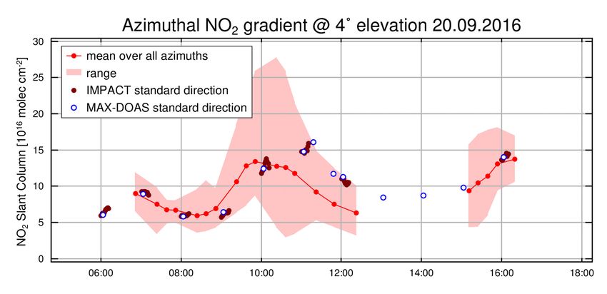
S3     Details on profile flagging

     Participants were allowed to submit flags, giving them the opportunity to mark profiles as invalid. Four participants submitted
     flags based on the following criteria:
          – BIRA/ bePRO: Profiles are considered valid if the retrieved degrees of freedom are > 1 and if the difference between
5           measured and modelled dSCDs is smaller than 30 %.
          – INTA: Profiles are valid if DOFS > 1 and if the RMSD between measured and simulated dSCDs is smaller than 1.5 times
            the daily averaged RMS.
          – KNMI: Profiles are invalid if the spread in the ensemble of solutions for AOT or the NO2 or HCHO tropospheric column
            is larger than 15 % of the retrieved value, or if there are less than 5 out of the ensemble of 20 retrievals for which a
10          solution was found.
          – MAPA: Flagging is based on a row of criteria (e.g. the agreement of modelled and measured dSCDs, implausible results
            or the consistency within the ensemble of possible solutions) with carefully chosen thresholds. A detailed description
            can be found in Beirle et al. (2019).

     Table S1 shows the statistics regarding the number of submitted profiles and the fraction of invalid profiles for all participants
     and species.

     Table S1. Submission and flagging statistics.

                                    HCHO              NO2 UV              NO2 Vis             Aerosol UV         Aerosol Vis
                                    Total Valid [%]   Total Valid [%]     Total Valid [%]     Total Valid [%]    Total Valid [%]
          bePRO       AUTHo         170      100       170         100    -       -           170    100         -       -
                      BIRAo         170      93        170          93    170     87          170    93          170     88
                      INTAo         170      78        170          75    170     71          170    87          170     80
          PRIAM       AIOFMol       170      100       170         100    -       -           170    100         -       -
                      BSUol         170      100       170         100    170     100         170    100         170     100
                      CMAol         169      100       169         100    169     100         169    100         169     100
                      MPICol        170      100       170         100    170     100         170    100         170     100
          HEPRO       IUPHDol       170      100       170         100    170     100         170    100         170     100
                      UTORol        -        -         170         100    170     100         170    100         170     100
          BOREAS      IUPBol        170      100       170         100    170     100         170    100         170     100
          M3          LMUo          170      100       170         100    170     100         170    100         170     100
          MMF         BIRAol        170      100       170         100    170     100         170    100         170     100
          Realtime    NASAa         170      100       170         100    170     100         -      -           170     100
          MARK        KNMIp         107      38        152          61    168     76          107    43          168     77
          MAPA        MPIC-1.0p     170      31        170          32    170     22          170    32          170     33
                      MPIC-0.8p     170      52        170          51    170     37          170    52          170     43

15

     S4     Further details on supporting observations

     S4.1    Aerosol extinction profiles

     The available raw data from the ceilometer are attenuated backscatter coefficient profiles β̃(h). For altitudes below 180 m, data
     are invalid due to insufficient overlap between sending and receiving telescope’s FOVs of the instrument, thus β̃(h < 180 m)

                                                                     5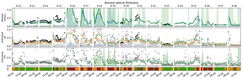
was set to β̃(h = 180 m). For profiles with simultaneously available sun photometer AOTs τs (λ), attenuated backscatter profiles
β̃(h) were converted to approximate backscatter profiles β(h), applying
h
Z
τs (λ = 1064 nm)
β(h) = β̃(h) · exp 2 R dh (1)
β̃(h0 )dh0
0
Extinction coefficient profiles αλ (h) at the MAX-DOAS retrieval wavelengths were then obtained by scaling of β(h) with the
5 sun photometer AOT according to:
τs (λ)
αλ (h) = R · β(h) (2)
β(h0 )dh0
Integrands with no specified limits in Eq. (1) and (2) indicate integration over the entire available profile. Values for τs (λ) at
the desired wavelengths were derived according to Eq. (4) in the main text. In case of missing sun photometer data, for instance
due to clouds, the MAX-DOAS retrieved AOT was used instead of τs . In this case no attenuation correction (Eq. (1)) could be
10 applied and the integration in Eq. (2) was performed over an averaging kernel smoothed profile (see main text Sect. 2.3.2), to
take into account the blindness of MAX-DOAS instruments for higher aerosol layers.
The resulting extinction coefficient profiles at 360 nm could partly be validated with Raman lidar observations at 355 nm
(the CESAR Water Vapor, Aerosol and Cloud lidar “CAELI”, operated within the European Aerosol Research lidar Network
(EARLINET, Bösenberg et al., 2003; Pappalardo et al., 2014) and described in detail in Apituley et al., 2009). Since for the
15 Raman lidar there is not sufficient telescope FOV overlap for altitudes < 1 km to retrieve reliable extinction profiles this
comparison is limited to the altitude range between 1 and 4 km. The average RMSD between scaled ceilometer and Raman
lidar profiles is ≈ 0.03. Table S2 summarizes the instrument’s properties. Figure S5 shows the available Raman lidar profiles in
comparison to the ceilometer derived profiles scaled with the respective sun photometer and MAX-DOAS AOT respectively.
Table S2. Properties of the two lidar instruments.
Instrument Raman lidar Ceilometer
Data product Aerosol extinction profile Elastic backscatter profile
Operational wavelength 355 nm 1064 nm
Altitude range 1 to 10 km 0.2 to 15 km
Vertical resolution 7.5 m 10 m
Temporal resolution 30 s 12 s
Data coverage 5 profiles between 13.9. and 15.9. Whole campaign
S4.2 Radiosonde flights
20 An overview of the radiosonde flights is given in Fig. S6. Example profiles are shown in the course of a comparison between
lidar and radiosonde observations in Supplement S4.5. Another preprocessing step of the sonde profiles shall be mentioned:
data quality was affected by calibrational drifting of the sensor, as it was optimized for low weight and cost rather than
performance. Even though a calibration against the CE-DOAS was performed directly before each launch, most profiles showed
a clear instrumental offset of about (1−2)×1010 molec cm−3 in the free troposphere. The offset was subtracted and the profiles
25 were subsequently rescaled to their initial surface concentration.
S4.3 NO2 lidar
The NO2 lidar provides profiles consisting of a series of altitude intervals or “boxes” with constant gas concentration between
a lower and an upper altitude limit. The conversion to profiles on the MAX-DOAS 200 m grid is demonstrated in Fig. S7. First,
6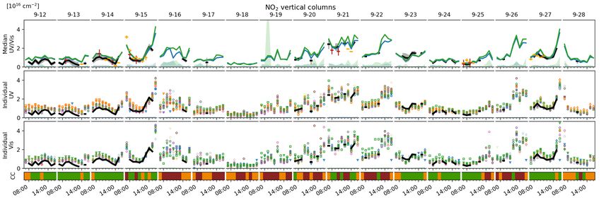
Figure S5. Comparison of the five available aerosol extinction profiles obtained from Raman lidar measurements (in black, with uncertainties
indicated by the grey areas) with AOT scaled ceilometer backscatter profiles. Scaling was performed with AOTs from sun photometer (blue)
and DOAS data (orange). In the last plot, lines show the mean deviation, whereas the borders of the couloured areas mark maximum and
minimum deviation.

Table S3. Overview over the radiosonde sampling flights shown in this study.

                                 Launch date        Flight timea [min]          Travel distancea [km]     Wind direction
                                  9-13 08:42                  10                             7                 SE
                                  9-14 09:03                  12                             5                 SE
                                  9-14 13:06                  14                             4                 SE
                                  9-15 08:04                  10                             8                  E
                                  9-15 10:25                  11                             8                 SE
                                  9-21 07:57                  12                            10                 SE
                                  9-21 10:14                  15                             5                 SE
                                  9-25 06:59                  17                             7                  S
                                  9-25 09:29                  12                            18                  S
                             a
                                 Only considering trajectory through the lowest 4 km of the atmosphere.

the boxes were converted to a continuous profile by linearly interpolating over box overlaps or gaps, which was then averaged
down to the 200 m MAX-DOAS retrieval grid resolution.

S4.4   Long path DOAS

                                                                                7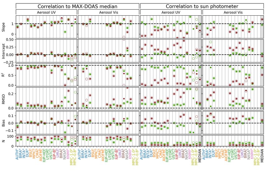
Figure S6. Sonde flight paths in the course of the campaign. Only data of the sonde ascent through the lowest 4 km of the atmosphere are
shown. Some flights shown here are not included in the comparison as they were launched before 6:30 h. The "minute" values in the legend
labels represent the flight time.

Figure S7. Regridding of an example NO2 lidar box profile (27 September 2016, 11:00) to the MAX-DOAS 200 m vertical resolution. In a
first step, gaps and overlaps within the box profile are linearly interpolated. The resulting profile is then averaged within the MAX-DOAS
retrieval layers.

                                                                    8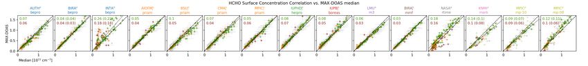
Figure S8. Setup of the LP-DOAS system. As shown on the map (Esri et al., 2018), the light sending and receiving telescope unit (left) was
located at 3.8 km distance to the meteorological tower (right), resulting in a total light path of 7.6 km. There were several retroreflectors
installed on the tower at different altitudes. However for this study, only the one at the very top (207 m altitude) was used to obtain the
average gas in the lowest retrieval layer, extending from 0 to 200 m altitude.

                                                                     9
S4.5 Consistency of supporting observations
The agreement of redundant supporting observations (processed as described in the main text Sect. 2.2) gives an impression
of their reliability and/ or representativeness. In the case of NO2 several observations of total vertical columns and surface
concentration (note again, that throughout this paper “surface concentration” refers to the average concentration in the lowest
5 retrieval layer) are available and compared in the correlation plots in Fig. S9 below. Corresponding time series plots are already
shown in the main text in Fig. 17 and 20, respectively. Tables S4 and S5 show the RMSD (as observed) and σ (the expected
deviation according to the specified measurement uncertainties) between each possible pair of observations. For the VCDs,
the RMSD is close to σ or below. A maximum RMSD of 1.5 σ is found between NO2 lidar and direct-sun DOAS. For the
surface concentrations however, there seem to be systematic deviations which split the observations into two pairs: radiosonde
10 and lidar observations agree well but are both systematically lower than LP-DOAS and tower measurements. MAX-DOAS UV
agrees better with LP-DOAS and tower observations, while MAX-DOAS Vis agrees more with sonde and lidar. Between the
LP-DOAS and the NO2 lidar, an RMSD of more than 4 σ is observed. There are several potential explanations:
1. Biases are introduced due to data processing (temporal and spatial regridding, for instance for the lidar profiles described
in Sect. S4.3).
15 2. Spatio-temporal variability of the real gas abundances
3. Imperfect estimates of the measurement uncertainties (in particular systematic deviations)
For the NO2 lidar and the radiosondes, there are four simultaneously recorded NO2 profiles available over the campaign
(simultaneous in the sense that for a single MAX-DOAS profile timestamp, profiles from both systems are available according
to the definitions in Sect. 2.2.3 in the main text). They are compared in the top row of Fig. S10. For the first situation, where
20 good spatial and temporal overlap is given, there is mostly an agreement within the specified errors. In the case of bad temporal
and/ or spatial overlap, strong deviations occur. For the 2nd and the 4th plot, there are several lidar profiles available, which
are temporally closer to the radiosonde (however further away from the corresponding MAX-DOAS profile), which in contrast
show very good agreement again. This shows that the real NO2 profile varies strongly even on timescales of ≈ 30 minutes
(see also (Peters et al., 2019)) and that improved synchronisation between MAX-DOAS and supporting observations should
25 be considered for future campaigns.
Table S4. Comparison of redundant measurements of the NO2 surface concentration (in 1011 molec cm−3 ). For each pair of observations,
the observed scatter (RMS) is compared to the specified uncertainty (σ).
Tower in-situ (0.56) Radiosonde (0.50) NO2 -Lidar (0.13)
RMSD σ RMSD σ RMSD σ
LP-DOAS (0.06) 0.32 0.56 1.01 0.51 0.57 0.13
NO2 -Lidar (0.13) 0.72 0.57 0.40 0.52 - -
Radiosonde (0.50) 0.99 0.78 - - - -
Table S5. Comparison of redundant measurements of the NO2 total columns (in 1016 molec cm−2 ). For each pair of observation, the
observed scatter (RMS) is compared to the specified uncertainty (σ).
Radiosonde (0.44) NO2 -Lidar (0.15)
RMSD σ RMSD σ
Direct-sun DOAS (0.23) 0.24 0.51 0.40 0.26
NO2 -Lidar (0.15) 0.34 0.48 - -
10Figure S9. Comparison of redundant supporting observations of NO2 VCDs (left panel) and surface concentration (right panel). MAX-
DOAS retrieved values are plotted in the background. To improve visibility, tower measurement uncertainties (vertical error bars of typically
(6.0 ± 0.5) × 1010 molec cm−3 ) are not shown.
11Figure S10. Top row: Comparison of NO2 lidar (orange) and radiosonde (red) profiles, that were assigned to a common MAX-DOAS
profile timestamp according to Sect. 2.2.3 in the main text. Dashed lines represent original instrument resolution while thick lines show
the concentrations averaged to the MAX-DOAS altitude grid. The colour of the dates indicates the cloud conditions. The rectangular little
subplots show a map (4 x 4 km) of the lidar line of sight and the sonde flight path. The dots on the sonde flight path mark the transitions
between the retrieval layers. The polar plot (to be read like a clock) shows the temporal overlap between the two observations, together with
the middle timestamps of each observation. Lower row: For the 2nd and 4th timestamp, there were lidar profiles available with improved
temporal overlap (however, with a worse overlap with the corresponding MAX-DOAS profile).
12S5 MAX-DOAS viewing distance
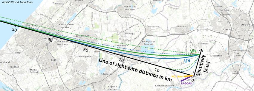
Wagner and Beirle (2016) derived polynomial relationships between the “horizontal sensitivity range” (HSR, defined as the
distance, at which the box airmass factors dropped to 1/e) and O4 differential airmass factors (dAMF). Applying this approach
to the CINDI-2 O4 dAMFs yields the HSRs shown in Fig. S12. A constant vertical O4 column of 1.19 · 1043 molec2 cm−5
5 was assumed. The HSR for the actually retrieved layers is more complicated and not assessed here, as information aspects
(which elevation contributes to information on which layer), geometrical limitations and the atmospheric state (trace gas and
aerosol layer height) would have to be taken into account. Depending on the conditions, HSRs vary between a few and tens
of kilometres (as shown in Fig. S11) defining whether only air masses over rural areas and/or urban areas (Gouda at 15 km
distance, Zoetermeer at 30 km distance and The Hague at 40 km distance. to the measurement site) are sampled. Further,
10 depending on the wind, plumes of Utrecht, Rotterdam or Amsterdam might be sampled.
13Figure S11. Line of sight of the MAX-DOAS instruments on a map (Esri et al., 2018). The coloured curves indicate the sensitivity for the
average (solid), the minimum (dashed) and maximum (dashed) viewing distances encountered during the campaign in the UV (blue) and Vis
(green).
Figure S12. Viewing distance (HSR) of MAX-DOAS instruments during CINDI-2. It was calculated for different elevation angles (1, 2, 3,
4, 5, 6 and 8◦ with increasing transparency of the curves) and the average value for UV and Vis (thick lines).
S6 Spatio-temporal mismatch and variability
Given the MAX-DOAS horizontal sensitivity ranges determined in Sect. S5, approximate values for the spatio-temporal mis-
match of MAX-DOAS and different supporting observations can be derived. They are given in Table S6. The potential impact
Table S6. Estimates for the average spatio-temporal mismatch of different supporting observations w.r.t. to the MAX-DOAS measurements.
For the location of the MAX-DOAS observations the centers of mass of the horizontal sensitivity curves from Sect. S5 were used. For the
location of sun photometer and direct-sun DOAS observations, the center of the lines of sight towards the sun up to 2 km atitude were
considered.
Observation Spatial mismatch [km] Temporal mismatch [min]
Sun photometer 13 8
Ceilometer 11 0
Direct-sun DOAS 13 23
NO2 -Lidar 10 9
Radiosonde 6 13
LP-DOAS 10 6
In-situ in tower 11 0
14of these mismatches can be demonstrated by means of the NO2 surface concentration. The left panel of Fig. S13 shows obser-
vations of the NO2 surface concentrations at their original temporal resolution ∆t and integration time tint . The CE-DOAS as
a point measurement with ∆t = tint = 1 min shows very strong variability on short timescales. However, for the tower mea-
surements (all in situ instruments in the tower vertically integrated as described in main text Sect. 2.2.5 at ∆t = 20 min and
5 tint ≈ 5 min), the LP-DOAS (∆t = 32 min, tint ≈ 100 s) there is already significant smoothing. The 1D-MAX-DOAS data
was recorded by DLR (see Supplement S10), who retrieved profiles in the nominal azimuth direction (287 ◦ ) more or less con-
tinuously (∆t = 15 min, tint ≈ 10 min). In all measurements there is significant variation on the sub-hour timescale. Further,
spatial variability might be observed in the form of disagreement between UV and Vis observations of the 1D-MAX-DOAS as
viewing distance and thus the sampled air volume changes between the two spectral ranges (see Supplement S5). To estimate
10 the order of magnitude, the right panel of Fig. S13 shows a kind of autocorrelation of the total campaign time series of each
observation. The RMSD between the original and a temporally shifted signal is calculated. 1D MAX-DOAS Vis data is not
shown, as multiple gaps in the data complicated the autocorrelation. Comparing this figure with values from Table S6 yields
that spatio-temporal variability causes RMSD values of around 3.5×10¹⁰ molec cm−3 in the NO2 surface concentration, which
is indeed of the order of the observed RMSD values in the NO2 surface concentration comparisons within this study (approx.
15 5 × 10¹⁰ molec cm−3 , compare to main text Fig. 22).
For another demonstration of the spatial variability, we refer to data from the IMPACT instrument (Peters et al., 2019),
an imaging MAX-DOAS operated by IUP-Bremen (IUPB) which allows to perform elevation "scans" in different azimuth
viewing directions in quick succession. During CINDI-2, the IMPACT performed full-azimuthal scans in 10◦ steps every 15
minutes. Figure S14 exemplarily shows the observed NO2 Vis dSCDs at 4◦ elevation on the 20 September 2016 together with
20 dSCDs measured by the IUPB standard MAX-DOAS instrument in the nominal azimuth direction (287◦ , compare main text
Sect. 2.1). The red shaded area depicts the variation of the dSCD with azimuth viewing direction. In particular around local
noon this variation is tremendous, exceeding a factor of five. Further investigation on this issue can be found in Peters et al.
(2019).
Figure S13. Left: Different observations of the NO2 surface concentrations on 14 September 2016, each at its original temporal resolution to
reveal short-term variations. Coloured areas behind the lines indicate the specified uncertainties. Right: RMSD values obtained from a kind
of autocorrelation analysis over the whole campaign (night times excluded). For each observation, the RMSD between the original and a
temporally shifted signal is calculated. The temporal shift (bottom horizontal axis) was varied between 0 and 4 hours. The temporal shift was
roughly converted to its spatial equivalent by multiplication with the average observed wind speed in the surface layer (≈ 5 m/s), yielding
the top horizontal axis.
15Figure S14. Variation in the NO2 Vis dSCDs with different azimuth viewing directions at 4◦ elevation, as observed by the IMPACT imaging
MAX-DOAS (Peters et al., 2019). Around local noon this variation is largest, exceeding a factor of 5. The time is UTC.
S7 Impact of the choice of pressure and temperature profiles for the RTMs
Pressure (p) and temperature (T ) profiles used for the RTMs within this study are averaged sonde measurements performed
in De Bilt by KNMI during September months of the years 2013-2015 (see main text Sect. 2.1.3). To estimate the effect of
this approximation on the results, IUPHD/ HEIPRO retrieved an additional set of profiles, using p and T information from
5 radiosondes launched at KNMI (De Bilt) during the campaign. Between one and three sondes were launched every day except
on 16 September. For each profile inversion, the temporally closest sonde observation was used. Table S7 shows the difference
in RMSD and Bias magnitude between these results and the "standard" results of IUPHD/ HEIPRO (that used the prescribed
averaged p and T profiles from years before) relative to the average RMSDs and average Bias magnitude for all participants.
The impact on the dSCD comparison is less than 5% for both, RMSDs and Bias magnitudes. For AOTs, VCDs and sur-
10 face concentrations, significant improvement (> 10 % in RMSD) is only observed for HCHO surface concentrations (17 %)
that contrasts with a deterioration for UV AOTs by 13%. The average improvement in RMSD for AOTs, VCDs and surface
concentrations is 3.2 %. The overall consistency between MAX-DOAS and supporting observations can thus be considered to
remain similar, despite larger changes in some Bias magnitudes are observed (up to 51 % improvement for NO2 Vis surface
concentrations and up to 20 % deterioration for UV AOTs).
Table S7. The differences in RMSDs and Bias magnitudes for the IUPHD/ HEIPRO results arising from using daily p and T profiles, relative
to the average RMSDs and Bias magnitudes assessed within the main study. Values are given for the comparisons of modelled and measured
dSCDs ("dSCDs") and the comparisons against the supporting observations of AOTs, VCDs and surface concentrations as described in the
main text. Minus signs indicate improvement. Only clear sky conditions were considered.
dSCDs AOT/VCD Surface
∆RMSD [%] ∆Bias [%] ∆RMSD [%] ∆Bias [%] ∆RMSD [%] ∆Bias [%]
HCHO 2.7 3.5 6.8 10.5 -17.4 -22.0
NO2 UV -0.7 -1.1 -2.7 -2.6 -3.5 8.7
NO2 Vis -0.7 -3.3 -0.8 -1.0 -2.8 -50.9
Aerosol UV -0.7 0.7 12.5 20.2 - -
Aerosol Vis -0.2 2.1 -8.7 -40.1 - -
16S8 Further details on the comparison results
S8.1 AVKs of individual participants
Figures S35 to S39 show the averaging kernels (AVKs) and retrieved degrees of freedom of signal (DOFS) of each participant
for aerosol UV. For explanation of colours and symbols please refer to main text Sect. 3.1. The DOFS values in brackets were
5 calculated considering valid data only.
Figure S15. Mean averaging kernels for Aerosol UV for each participant. Coloured values at AVK peaks show the amount of retrieved
information on the respective layer in percent. "DOFS" numbers are given for clear-sky (green) and cloudy (red) conditions. Values in
brackets are DOFS including flagging.
17Figure S16. Mean averaging kernels for Aerosol Vis for each participant. Description of Fig. S35 applies.
18Figure S17. Mean averaging kernels for HCHO for each participant. Description of Fig. S35 applies.
19Figure S18. Mean averaging kernels for NO2 UV for each participant. Description of Fig. S35 applies.
20Figure S19. Mean averaging kernels for NO2 Vis for each participant. Description of Fig. S35 applies.
21S8.2 Profile deviation statistics
Figures S20 to S24 show statistics on the observed differences in the retrieved profiles for all five species. The plots on the
left compare the retrieved profiles of individual participants x to the median MAX-DOAS profiles x̄. While the vertical axes
represent altitude, the horizontal axes depicts the difference x − x̄. The coloured boxes indicate the 25 % − 75 % percentile,
5 whiskers are 5 % − 95 %. Black dots indicate the mean value. For each layer there are boxplots for clear-sky (green) and
cloudy conditions (red). Note that for aerosol there are two different horizontal axes defined for the two cloud conditions: the
green scale at the bottom and the red scale on the top of each plot. Only valid data (flagged) was considered. For aerosol and
NO2 a plot on the very right shows statistics of the difference of supporting measurements xanc (lidar/ radiosonde for NO2 ,
sun photometer scaled ceilometer for aerosol) to the median x̄, hence xanc − x̄. The numbers in all the plots show RMSD
10 deviation of the three lowest (most sensitive) layers. Dashed lines indicate the median retrieval uncertainty as specified by the
participants.
Figure S20. Left: Deviations of Aerosol UV profiles (valid only) of individual participants from the MAX-DOAS median profiles. Dots
show the mean, boxes indicate the (25 %-75 %) percentile, and whiskers show (25 %-75 %) percentile. Green (red) box-whiskers represent
clear (cloudy) conditions. Note, that there are different x-scales (on top and bottom of the plot) for different cloud conditions. The average
standard deviations specified by the participants are indicated by the dashed lines. Right: Deviation of the AOT scaled ceilometer backscatter
signal to the MAX-DOAS median profiles. The numbers in the plots indicate RMSD values for clear sky (green) and cloudy (red) conditions.
Further details are given in the related text in Sect. S8.2
22Figure S21. Deviations of Aerosol Vis profiles (valid only) of individual participants from the MAX-DOAS median profiles. Description of
Fig. S20 applies.
Figure S22. Deviations of HCHO profiles (valid only) of individual participants from the MAX-DOAS median profiles. The description of
Fig. S20 applies but for HCHO, there is no independent reference profile available.
23Figure S23. Deviations of NO2 UV profiles (valid only) of individual participants from the MAX-DOAS median profiles. The description
of Fig. S20 applies. On the right, deviation of the median retrieved profiles from the few available NO2 lidar and sonde profiles are shown.
Figure S24. Deviations of NO2 Vis profiles (valid only) of individual participants from the MAX-DOAS median profiles. The description of
Fig. S23 applies.
24S8.3 Correlation plots for AOTs, VCDs and surface concentrations
Figures S25 to S32 show the individual correlation plots for the comparisons of AOTs, VCDs and surface concentrations as summarized in Sect.
3.4, 3.5 and 3.6 in the main text, respectively. The colours indicate cloud conditions: clear-sky (green) and cloudy conditions (red). Transparent
markers represent data points flagged as invalid. The small grey bars indicate uncertainties in the measurement. For the median values, the bars
5 show the standard deviation among the participants (valid data only). Dashed lines in the correlation plots represent the ideal 1:1 line. Correlations
were performed separately against MAX-DOAS median values and supporting observations. For AOTs a third correlation is shown for the partial
AOT (with PAC applied).
25
Figure S25. Correlation of Aerosol UV AOTs. Complementary to main text Sect. 3.426
Figure S26. Correlation of Aerosol Vis AOTs. Complementary to main text Sect. 3.4
Figure S27. HCHO VCD correlation plots. Complementary to main text Sect. 3.5Figure S28. NO2 UV VCD correlation plots. Complementary to main text Sect. 3.5
27
Figure S29. NO2 Vis VCD correlation plots. Complementary to main text Sect. 3.5
Figure S30. HCHO surface concentration correlation plots. Complementary to main text Sect. 3.6Figure S31. NO2 UV surface concentration correlation plots. Complementary to main text Sect. 3.6
28
Figure S32. NO2 Vis surface concentration correlation plots. Complementary to main text Sect. 3.6S9 Impact of smoothing on surface concentration
For NO2 the impact of smoothing effects on the surface concentration retrieved by OEM algorithms can be estimated from
profiles of the NO2 lidar and radiosondes. Each profile is smoothed according to Eq. (9) in the main text and the difference
in surface concentration between the smoothed and the unsmoothed profile is calculated. Fig. S33 shows histograms of the
5 calculated differences. The standard deviation is about 5 × 10⁹ molec cm−3 which is only about 10 % of the total average
RMSD between MAX-DOAS and LP-DOAS observations. An estimate of the impact of smoothing on the retrieval results is
actually provided by the OEM retrievals themselves as the "smoothing error". The specified smoothing errors are also indicated
in Fig. S33 and are similar to the standard deviation observed in in this test, meaning that for the surface layer they are well
representative for the real impact of smoothing.
Figure S33. Histograms of the observed deviations in surface concentration between raw and smoothed lidar/ radiosonde NO2 profiles. Solid
and dashed lines indicate mean value and standard deviation, respectively. Coloured areas represent the median smoothing errors as specified
by the OEM retrievals, which is in good agreement with the deviations obtained from the supporting NO2 profiles.
10 S10 Participant’s own dSCD comparison results
This section shows the comparison results for the case where each participant uses dSCDs measured with his own instrument.
Evaluation and plots are fully equivalent to Sect. 3 in the main text. With DLR (German Aerospace Center, Oberpfaffenhofen,
Germany, marked by blue squares) and USTC (University of Science and Technology of China, Hefei, China, marked by green
squares), two other participants were included here, retrieving profiles with bePRO and HEIPRO, respectively. Gaps in the data
15 are mostly related to instrument malfunction during the campaign. Further, not all instruments covered the spectral range to
detect all desired species and the corresponding participants therefore do not appear in the respective plots.
S10.1 Information content
Information on the averaging kernels and DOFS. This section is equivalent to Sect. S10.1 in the main text and Sect. S8.1 in
this supplement, respectively.
29Figure S34. Average AVKs for the retrieved species (median over participants, mean over time). Each altitude and corresponding AVK
line are associated with a colour, which is defined by the colour of the corresponding altitude-axis label. The dots mark the AVK diagonal
elements. The number next to the dots show the exact value in percent, which corresponds to the amount of retrieved information on the
respective layer. In the upper right of each panel, the DOFS (median among institutes, average over time) are given for clear-sky (green) and
cloudy conditions (red).
30Figure S35. Mean averaging kernels for Aerosol UV for each participant retrieving from their own dSCDs. Coloured values at AVK peaks
show the amount of retrieved information on the respective layer in percent. "DOFS" numbers are given for clear-sky (green) and cloudy
(red) conditions. Values in brackets are DOFS including flagging.
31Figure S36. Mean averaging kernels for Aerosol Vis for each participant. Description of Fig. S35 applies.
32Figure S37. Mean averaging kernels for HCHO for each participant. Description of Fig. S35 applies.
33Figure S38. Mean averaging kernels for NO2 UV for each participant. Description of Fig. S35 applies.
34Figure S39. Mean averaging kernels for NO2 Vis for each participant. Description of Fig. S35 applies.
35S10.2 Overview plots
This section is equivalent to Sect. 3.2 in the main text.
3637
Figure S40. Aerosol UV extinction profiles retrieved from the participant’s own dSCDs. The lowest row shows AOT scaled ceilometer backscatter profiles, calculated
as described in Sect. S4.1. Backscatter profiles, which were scaled from MAX-DOAS AOTs (and which are therefore not fully independent) are marked by pink
triangles. Maximum extinction values reach 20 km−1 , exceeding the colour scale.38
Figure S41. Aerosol Vis extinction profiles retrieved from the participant’s own dSCDs. The lowest row shows AOT scaled ceilometer backscatter profiles, calculated
as described in Sect. S4.1. Backscatter profiles, which were scaled from MAX-DOAS AOTs (and which are therefore not fully independent) are marked by pink
triangles. Maximum extinction values reach 20 km−1 , exceeding the colour scale.39
Figure S42. HCHO concentration profiles retrieved from the participant’s own dSCDs. The "Surf"-row shows LP-DOAS surface concentrations.40
Figure S43. NO2 UV concentration profiles retrieved from the participant’s own dSCDs. The lowest row shows a combined dataset of NO2 lidar, radiosonde,
LP-DOAS and tower in-situ data. Redundant surface concentration measurements were averaged.41
Figure S44. NO2 Vis concentration profiles retrieved from the participant’s own dSCDs. The lowest row shows a combined dataset of NO2 lidar, radiosonde,
LP-DOAS and tower in-situ data. Redundant surface concentration measurements were averaged.S10.3 Modelled and measured dSCDs
This section is equivalent to Sect. S10.3 in the main text.
Figure S45. O4 UV dSCD correlation when profiles are retrieved from the participant’s own dSCDs. Marker colours and marker shapes
indicate the cloud conditions and viewing elevation angles, respectively. Numbers represent the measurement error weighted RMSD between
measured and modelled dSCDs for clear sky (green) and cloudy (red) conditions. Values in brackets were calculated only considering valid
data.
42Figure S46. O4 Vis dSCD correlation. Legends of Fig. S45 apply.
Figure S47. HCHO dSCD correlation. Legends of Fig. S45 apply.
43Figure S48. NO2 UV dSCD correlation. Legends of Fig. S45 apply.
Figure S49. NO2 Vis dSCD correlation. Legends of Fig. S45 apply.
44S10.4 Aerosol optical thickness (AOT)
This section is equivalent to Sect. S10.4 in the main text.
Figure S50. MAX-DOAS AOTs retrieved from the participant’s own dSCDs in comparison to sun photometer data. Symbol and symbol
colours are chosen according to Table 2 in the main text. Transparent symbols indicate data flagged as invalid. Top row: MAX-DOAS median
results vs. the available supporting observations, according to the legend below the plot. The "institute scatter" areas show the scattering
among the participants in terms of standard deviation with valid data considered only. Two lower rows: Comparison of the individual
participants for the two spectral retrieval ranges. Here the coloured area is the average retrieval error, as specified by the participants.
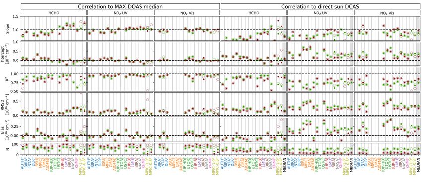
45Figure S51. Correlation statistics for AOTs. The two left columns give an impression on the agreement among the institutes, as they show
the correlation of the individual participant’s retrieved AOT (ordinate of the underlying correlation plot) against the median (abscissa). The
two right columns show the correlation against the sun photometer AOT (partial AOT in the case of OEM retrievals) instead of the median.
Green and red symbols represent cloud-free and cloudy conditions, respectively. Hollow circles represent values for all submitted data, the
dots only consider data points flagged as valid. N is the number of profiles which contributed to the respective data points above. The total
number of submitted profiles per participant and species were 170. On the right also the correlation between the MAX-DOAS median results
and supporting observations are included (grey shaded columns).
S10.5 Trace gas vertical column densities (VCDs)
This section is equivalent to Sect. S10.5 in the main text.
46Figure S52. Comparison of MAX-DOAS HCHO VCDs retrieved from the participant’s own dSCDs vs. direct-sun DOAS, NO2 lidar and
radiosonde. Descriptions of Fig. S50 apply.
Figure S53. Comparison of MAX-DOAS NO2 VCDs retrieved from the participant’s own dSCDs vs. direct-sun DOAS. Descriptions of Fig.
S50 apply.
47Figure S54. Correlation statistics of trace gas VCDs retrieved from the participant’s own dSCDs. Legends and description of Fig. S51 apply.
48S10.6 Trace gas surface concentrations
This section is equivalent to Sect. S10.6 in the main text.
Figure S55. Comparison of MAX-DOAS HCHO surface concentrations retrieved from the participant’s own dSCDs. Description of Fig.
S50 applies.
Figure S56. Comparison of MAX-DOAS NO2 surface concentrations retrieved from the participant’s own dSCDs. Description of Fig. S50
applies.
49Figure S57. Correlation statistics of trace gas surface concentrations retrieved from the participant’s own dSCDs. Basic description of Fig.
S51 applies.
5051
Figure S58. Summary of the comparisons in Sect. S10 for clear-sky conditions. Left panel shows RMSD, right panel shows Bias. Average values of RMSD (Bias)
define the colour scale of each column of the left (right) panel as indicated by the color bars on the top left (top right) of the figure. Values of AOT, VCD and
surface concentration are given with respect to the corresponding supporting observations. White spaces indicate no data. Average observed values (bottom row)
are rounded campaign averages of the supporting observations. Average Bias and Average Bias magnitude values (third last and second last row of right panel)
represent the averages over the signed and the absolute Bias values, respectively. The "data used"-column in the center indicates which fraction of the maximum
number (170) of available profiles has been used. Participants who submitted flags are represented by two rows: one considering all data and one using only those
flagged as valid ("valid only").References
Apituley, A., Wilson, K., Potma, C., Volten, H., and de Graaf, M.: Performance Assessment and Application of Caeli–A highperformance Ra-
man lidar for diurnal profiling of Water Vapour, Aerosols and Clouds, in: Proceedings of the 8th International Symposium on Tropospheric
Profiling, pp. 19–23, S06-O10-1-4, Delft/KNMI/RIVM Delft, Netherlands, 2009.
5 Beirle, S., Dörner, S., Donner, S., Remmers, J., Wang, Y., and Wagner, T.: The Mainz profile algorithm (MAPA), Atmospheric Measurement
Techniques, 12, 1785–1806, https://doi.org/10.5194/amt-12-1785-2019, https://www.atmos-meas-tech.net/12/1785/2019/, 2019.
Bösenberg, J., Matthias, V., Amodeo, A., Amoiridis, V., Ansmann, A., Baldasano, J. M., Balin, I., Balis, D., Böckmann, C., Boselli, A.,
Carlsson, G., Chaikovsky, A., Chourdakis, G., Comeron, A., Tomasi, F. D., Eixmann, R., Freudenthaler, V., Giehl, H., Grigorov, I.,
Hagard, A., Iarlori, M., Kirsche, A., Kolarov, G., Komguem, L., S. Kreipl, W. K., Larcheveque, G., Linné, H., Matthey, R., Mattis, I.,
10 Mekler, A., Mironova, I., Mitev, V., Mona, L., Müller, D., Music, S., Nickovic, S., Pandolfi, M., Papayannis, A., Pappalardo, G., Pelon,
J., Perez, C., Perrone, R., Persson, R., Resendes, D. P., Rizi, V., Rocadenbosch, F., Rodrigues, J. A., Sauvage, L., Schneidenbach, L.,
Schumacher, R., Shcherbakov, V., Simeonov, V., Sobolewski, P., Spinelli, N., Stachlewska, I., Stoyanov, D., Trickl, T., Tsaknakis, G.,
Vaughan, G., Wandinger, U., Wang, X., Wiegner, M., Zavrtanik, M., and Zerefos, C.: EARLINET: A European Aerosol Research Lidar
Network to establish an aerosol climatology, Report 348, ISSN 0937-1060, 192 pp., Max-Planck-Institut für Meteorologie, 2003.
15 Chan, K. L., Wang, Z., Ding, A., Heue, K.-P., Shen, Y., Wang, J., Zhang, F., Hao, N., and Wenig, M.: MAX-DOAS measurements of
tropospheric NO2 and HCHO in Nanjing and the comparison to OMI observations, Atmospheric Chemistry and Physics Discussions,
2019, 1–25, https://doi.org/10.5194/acp-2018-1266, https://www.atmos-chem-phys-discuss.net/acp-2018-1266/, 2019.
Clémer, K., Van Roozendael, M., Fayt, C., Hendrick, F., Hermans, C., Pinardi, G., Spurr, R., Wang, P., and De Mazière, M.: Multiple
wavelength retrieval of tropospheric aerosol optical properties from MAXDOAS measurements in Beijing, Atmospheric Measurement
20 Techniques, 3, 863–878, https://doi.org/10.5194/amt-3-863-2010, https://www.atmos-meas-tech.net/3/863/2010/, 2010.
Esri, EsriNL, Rijkswaterstaat, Intermap, NASA, NGA, Kadaster, U. ., Esri, HERE, Garmin, P, I., and METI: arcGIS World Topo Map, 2018.
Mayer, B. and Kylling, A.: Technical note: The libRadtran software package for radiative transfer calculations - description and examples of
use, Atmospheric Chemistry and Physics, 5, 1855–1877, https://doi.org/10.5194/acp-5-1855-2005, https://www.atmos-chem-phys.net/5/
1855/2005/, 2005.
25 Ortega, I., Berg, L. K., Ferrare, R. A., Hair, J. W., Hostetler, C. A., and Volkamer, R.: Elevated aerosol layers modify the O2–O2
absorption measured by ground-based MAX-DOAS, Journal of Quantitative Spectroscopy and Radiative Transfer, 176, 34 – 49,
https://doi.org/https://doi.org/10.1016/j.jqsrt.2016.02.021, http://www.sciencedirect.com/science/article/pii/S0022407315301746, 2016.
Pappalardo, G., Amodeo, A., Apituley, A., Comeron, A., Freudenthaler, V., Linné, H., Ansmann, A., Bösenberg, J., D’Amico, G., Mattis, I.,
Mona, L., Wandinger, U., Amiridis, V., Alados-Arboledas, L., Nicolae, D., and Wiegner, M.: EARLINET: towards an advanced sustainable
30 European aerosol lidar network, Atmospheric Measurement Techniques, 7, 2389–2409, https://doi.org/10.5194/amt-7-2389-2014, https:
//www.atmos-meas-tech.net/7/2389/2014/, 2014.
Peters, E., Ostendorf, M., Bösch, T., Seyler, A., Schönhardt, A., Schreier, S. F., Henzing, J. S., Wittrock, F., Richter, A., Vrekoussis, M.,
and Burrows, J. P.: Full-azimuthal imaging-DOAS observations of NO2 and O4 during CINDI-2, Atmospheric Measurement Techniques
Discussions, 2019, 1–30, https://doi.org/10.5194/amt-2019-33, 2019.
35 Wagner, T. and Beirle, S.: Estimation of the horizontal sensitivity range from MAX-DOAS O4 observations, Tech. rep., QA4ECV, http:
//www.qa4ecv.eu/sites/default/files, 2016.
Wagner, T., Deutschmann, T., and Platt, U.: Determination of aerosol properties from MAX-DOAS observations of the Ring effect, Atmo-
spheric Measurement Techniques, 2, 495–512, https://doi.org/10.5194/amt-2-495-2009, https://www.atmos-meas-tech.net/2/495/2009/,
2009.
40 Wagner, T., Beirle, S., Benavent, N., Bösch, T., Chan, K. L., Donner, S., Dörner, S., Fayt, C., Frieß, U., García-Nieto, D., Gielen, C.,
González-Bartolome, D., Gomez, L., Hendrick, F., Henzing, B., Jin, J. L., Lampel, J., Ma, J., Mies, K., Navarro, M., Peters, E., Pinardi,
G., Puentedura, O., Puk, ı̄te, J., Remmers, J., Richter, A., Saiz-Lopez, A., Shaiganfar, R., Sihler, H., Van Roozendael, M., Wang, Y., and
Yela, M.: Is a scaling factor required to obtain closure between measured and modelled atmospheric O4 absorptions? An assessment
of uncertainties of measurements and radiative transfer simulations for 2 selected days during the MAD-CAT campaign, Atmospheric
45 Measurement Techniques, 12, 2745–2817, https://doi.org/10.5194/amt-12-2745-2019, https://www.atmos-meas-tech.net/12/2745/2019/,
2019.
52You can also read