Spatial Heterogeneity Analysis: Introducing a New Form of Spatial Entropy
←
→
Page content transcription
If your browser does not render page correctly, please read the page content below
entropy
Article
Spatial Heterogeneity Analysis: Introducing a New
Form of Spatial Entropy
Chaojun Wang and Hongrui Zhao *
 3S Center, Tsinghua University; Institute of Geomatics, Department of Civil Engineering, Tsinghua University,
 Beijing 100084, China; wangcj16@mails.tsinghua.edu.cn
 * Correspondence: zhr@mail.tsinghua.edu.cn; Tel.: +86-010-62794976

 Received: 26 April 2018; Accepted: 18 May 2018; Published: 23 May 2018

 Abstract: Distinguishing and characterizing different landscape patterns have long been the primary
 concerns of quantitative landscape ecology. Information theory and entropy-related metrics have
 provided the deepest insights in complex system analysis, and have high relevance in landscape
 ecology. However, ideal methods to compare different landscape patterns from an entropy view are
 still lacking. The overall aim of this research is to propose a new form of spatial entropy (Hs ) in order
 to distinguish and characterize different landscape patterns. Hs is an entropy-related index based on
 information theory, and integrates proximity as a key spatial component into the measurement of
 spatial diversity. Proximity contains two aspects, i.e., total edge length and distance, and by including
 both aspects gives richer information about spatial pattern than metrics that only consider one aspect.
 Thus, Hs provides a novel way to study the spatial structures of landscape patterns where both
 the edge length and distance relationships are relevant. We compare the performances of Hs and
 other similar approaches through both simulated and real-life landscape patterns. Results show that
 Hs is more flexible and objective in distinguishing and characterizing different landscape patterns.
 We believe that this metric will facilitate the exploration of relationships between landscape patterns
 and ecological processes.

 Keywords: information entropy; landscape configuration; thermodynamics; spatial diversity; proximity

1. Introduction
     Distinguishing and characterizing different landscape patterns are among the primary concerns of
quantitative landscape ecology, since the distributions of energy, material, and species in landscapes are
determined by specific patterns [1–5]. Landscape patterns are characterized by both their composition
and their configuration, which collectively define landscape structure [6,7]. The interplay between
landscape patterns and ecological processes is profoundly important, with patterns constraining
processes and processes creating patterns in a reciprocal feedback [8–10]. Therefore, accurately
capturing and characterizing landscape patterns are the key foundations for most analysis in landscape
ecology [3,9].
     Among all of the fields of natural sciences, the field of information theory and entropy-related
metrics have provided the deepest insights into complex system analysis, and have high relevance
in landscape ecology [10–13]. Descriptions of landscape patterns, dynamics of ecological processes,
and interactions of pattern-process across scales in space and time are all constrained by entropy and the
second law of thermodynamics [10]. The form of the entropy concept that is widely used in landscape
ecology was proposed by Shannon in the 1940s [14]. Shannon entropy (also called information
entropy) is a quantitative measure of the diversity and information content of a signal, and it has
formed the cornerstone of information theory [15]. After its origination, Shannon entropy was rapidly
introduced to the field of landscape ecology (e.g., see literature [16,17]). Several researchers have

Entropy 2018, 20, 398; doi:10.3390/e20060398                                    www.mdpi.com/journal/entropy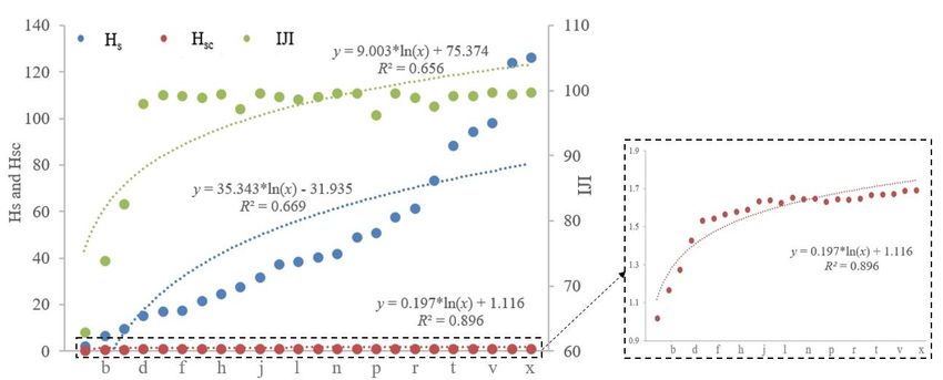
Entropy 2018, 20, 398                                                                                2 of 13

explored how Shannon’s quantitative theory principles can be applied to space (see literature [2,18–22]).
The challenge of this extension of Shannon entropy to spatial analysis is due to the fact that space is
a specific form of multi-dimensional system where the different dimensions are intimately linked [23],
while information systems that were studied by Shannon are made of messages decomposed into
one-dimensional signals [24]. These heuristic studies have clarified some quantitative aspects of
landscape patterns. However, one intriguing question is whether or not the notion of diversity that
is defined in information theory is influenced by some of the fundamental properties that space
generates and conveys [23]. More specifically, when Shannon entropy is applied in space, the problem
of dimension mismatch occurs [25].
      Fortunately, to date, at least two alternative approaches have been developed to solve this
problem. The first was proposed by Claramunt [23]. This approach is extended from Shannon entropy,
and derived from the principles of the Tobler’s First law (TFL) in geography. Claramunt’s seminal
work is thought-provoking, and it differs from conventional methods by modeling distance as a key
factor that influences the way that similar or different entities are interrelated in space [23]. Thus,
this entropy-related measure can effectively distinguish different landscape patterns to some degree.
However, our experience using this approach shows that it is quite complicated since several kinds of
distance need to be calculated. Moreover, as many scholars have argued, distance is not always the
key factor that relates to entities in space (please refer to [26–28]).
      The second approach is based on Boltzmann entropy (also called configuration entropy). Cushman
has proposed that the entropy of a landscape mosaic can be calculated using the Boltzmann
equation, with entropy equals to the natural logarithm of the number of unique configurations of
a landscape (microstates), which has the same total edge length (macrostate) as the focal landscape [3].
This approach can also distinguish different landscape patterns with various macrostates, and it
provides a means to understand the relationships between entropy and landscape configurations.
However, as the dimensionality and number of categories increase (e.g., realistic landscapes), the
number of unique configurations rapidly becomes intractably large, which makes it impossible to
calculate the configuration entropy. At the same time, as the dimensionality and the number of
categories increase, the number of potential macrostates (i.e., total edge length) also increases extremely
rapidly, which makes the calculation more complicated. More importantly, the assumption behind this
approach, that true thermodynamic relationships between landscape configuration and entropy, is
still questionable.
      Thus, methods that effectively describe and distinguish different landscape patterns from
an entropy perspective are still lacking. The overall aim of this paper is to propose a new form
of spatial entropy (Hs ), which can be used to distinguish and characterize different landscape patterns.
Hs is an entropy-related index based on information theory, and it integrates proximity as the key factor
that relates entities in geo-space. Proximity has been recognized as the central organizing principle in
space [27,28], and contains two aspects, including edge length and distance. In this way, Hs provides
a novel way to study spatial structures of landscape patterns where categories and proximity are both
relevant to the analysis. We tested the performance of Hs and other similar approaches based on
both simulated and real-life landscapes, and our results show that Hs is more flexible and sensitive in
characterizing and distinguishing different landscape patterns.

2. Methods
     The central focus on spatial heterogeneity has been widely recognized as the salient characteristics
of landscape ecology [4], and distinguishing different landscape patterns is the first step in the analysis
of spatial heterogeneity. Obviously, Shannon entropy, as discussed above, does not provide sufficient
information in spatial analysis since it only captures the compositional information (i.e., richness and
evenness) of landscapes, and it ignores the configurational information (see Figure 1 as an example).
What would be more useful is to measure the entropy of different landscape patterns at a particular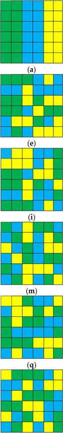
Entropy 2018, 20, 398 3 of 13
number of classes, and proportionality of each class [3]. Thus, a fundamental question needs to be
addressed, is how
Entropy 2018, 20, x to evaluate the role that is played by space? 3 of 13
Figure 1. Eight possible configurations (a–h) of a landscape mosaic with dimensions 3 × 3, two classes,
Figure 1. Eight possible configurations (a–h) of a landscape mosaic with dimensions 3 × 3, two classes,
5 cells of class A, and 4 cells of class B, the length and width of each cell are unit size. Landscapes (a–h)
5 cells of class A, and 4 cells of class B, the length and width of each cell are unit size. Landscapes (a–
show different patterns, however, have the same Shannon entropy since all of them contain the same
h) show different patterns, however, have the same Shannon entropy since all of them contain the
compositional information (based on descriptions and discussions in [3]).
same compositional information (based on descriptions and discussions in [3]).
In
In order
order to to quantitatively
quantitatively measure
measure the the influence
influence of of space,
space, thethe fundamental
fundamental properties
properties thatthat space
space
generates and conveys should be considered. Similarly, to the definition
generates and conveys should be considered. Similarly, to the definition in the context of information in the context of information
theory,
theory,aaspatial
spatialmeasure
measureofofdiversity
diversityshould
should take
takeinfluence
influence of of
space
spaceintointo
account
accountwhen
whenconsidering
considering the
degree of uncertainty in selecting some entities of
the degree of uncertainty in selecting some entities of interest [23]. interest [23].
The
The First
First Law
Law ofof Geography
Geography (also called Tobler’s
(also called Tobler’s FirstFirst Law,
Law, TFL)
TFL) maymay help
help to
to solve
solve this
this problem
problem
and
and to to bridge
bridge thethe gaps
gaps between
between Shannon
Shannon entropyentropy and and aa wayway thatthat diversity
diversity would
would be be evaluated
evaluated in in
space. This law states that “Everything is related to everything else, but
space. This law states that “Everything is related to everything else, but near things are more related near things are more related
than
than distant
distant things”
things” [29],
[29], and
and it has resonated
it has resonated strongly
strongly in in geography
geography since since near
near and related are
and related are useful
useful
concepts
concepts at the core of spatial analysis and modeling [26,28]. However, the concepts of near and
at the core of spatial analysis and modeling [26,28]. However, the concepts of near and
related
related werewerevaguely
vaguelydefined
definedby byTobler,
Tobler, which
which hashasledledto atolot of controversies
a lot of controversies about whatwhat
about is near and
is near
what
and whatis related in practical
is related applications
in practical (see [27]).
applications Recently,
(see [27]). more and
Recently, more more
andscholars, including
more scholars, Tobler
including
himself, tend to use the concept of “proximity” to measure the nearness
Tobler himself, tend to use the concept of “proximity” to measure the nearness between entities between entities in space [30].
in
Proximity contains two factors, including the total edge length (it measures
space [30]. Proximity contains two factors, including the total edge length (it measures the total the total amount of edges
between
amount of different
edges classes
betweenindifferent
a landscape, classessee in
[3])aand distance,see
landscape, and it is
[3]) a more
and flexible
distance, andandit ispowerful
a more
concept in spatial analysis and modeling. Specifically, proximity
flexible and powerful concept in spatial analysis and modeling. Specifically, proximity is proportional to the total edgeis
length between
proportional to the
the different
total edgeclasses
lengthand is inversely
between proportional
the different classestoand theisdistance
inverselybetween different
proportional to
class centers between
the distance in space different
[28]. Taking class Figure
centers 1 as
in an example,
space these eight
[28]. Taking Figure different configurations
1 as an example, have
these eight
the same Shannon entropy, however, their proximity information
different configurations have the same Shannon entropy, however, their proximity information are various (e.g., the total edge
are
length
variousof(e.g.,
landscapes
the total a–c
edgeare 5, 6, 9; and,
length the distance
of landscapes a–cbetween
are 5, 6,different
9; and, the class centersbetween
distance are 1.35, different
0.9, 0.45,
respectively).
class centers are Intuitively,
1.35, 0.9,proximity contains richer
0.45, respectively). information
Intuitively, proximity(bothcontains
edge length
richerand distance), and
information (bothit
seems to be an efficient tool to measure the role that is played by space.
edge length and distance), and it seems to be an efficient tool to measure the role that is played by
space. Thus, through the introduction of proximity, a new form of spatial entropy (Hs ) can be developed
that will
Thus,better quantify
through spatial heterogeneity
the introduction of proximity, (or diversity,
a new form as heterogeneity may be regarded
of spatial entropy (Hs) can be as
an essentialthat
developed cause andbetter
will a consequence of diversity
quantify spatial in the context
heterogeneity (or of landscape
diversity, as ecology, please may
heterogeneity see [9]).
be
This idea rests on two general and objective assumptions: on the one
regarded as an essential cause and a consequence of diversity in the context of landscape ecology, hand, the entropy of a landscape
should
please see not[9]).
only reflect
This idea the
restscompositional
on two generalcharacteristics of entities, but
and objective assumptions: onalso the spatial
the one hand, the structures
entropy
of
of atheir distributions;
landscape should not on the
onlyother
reflecthand, such an extension
the compositional of Shannon
characteristics entropy but
of entities, should
also reflect our
the spatial
structures of their distributions; on the other hand, such an extension of Shannon entropy should
reflect our intuitions when perceiving the configurational properties (i.e., disorder) of a landscape. It
also should be noted that, as TFL implies, in closed spatial systems, interactions between different
entities occur within the represented space. However, there are no such limitations for an open spatial
system, and the evaluation of spatial diversity would be far more complex when compared to closed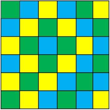
Entropy 2018, 20, 398                                                                                4 of 13

intuitions when perceiving the configurational properties (i.e., disorder) of a landscape. It also should
be noted that, as TFL implies, in closed spatial systems, interactions between different entities occur
within the represented space. However, there are no such limitations for an open spatial system, and the
evaluation of spatial diversity would be far more complex when compared to closed systems [31].
This study focuses on closed spatial systems, and it explores a way that spatial diversity would be
measured given a particular number of classes, and proportionality of each class. Based on these
assumptions, a new form of spatial entropy can be defined, as follows:
                                                     n
                                                           Li
                                         Hs = − ∑             p log2 pi                                 (1)
                                                    i =1
                                                           di i

                                                           n
                                            Li =           ∑    Lik                                     (2)
                                                      k=1
                                                      i 6= k
                                                           n
                                             di =          ∑    dik                                     (3)
                                                      k=1
                                                      i 6= k

where n is the number of different classes and pi denotes the proportionality of class i in a landscape.
Li is the total amount of edges between class i and other different classes (or patch types), and it equals
to the sum of lengths of all edge segments involving the corresponding class [32]. di denotes the sum
of average distances between the different class centers. It should be noted that the distance that is
considered in Hs might be any form that fulfils the metric properties of distance (e.g., Manhattan
distance, Euclidean distance, contextual distance, cognitive distance). In this study, we consider the
Euclidean distance in its application to geographical space. When different class centroids coincide, di
can be taken as a relatively small constant (such as 0.5-unit length) in order to avoid the “noise” effect
of null values in the calculations.
      As mentioned above, Hs explicitly models proximity as a key factor that relates entities in space,
and it builds the bridge between Shannon entropy and a way that diversity (or heterogeneity) would
be evaluated in spatial analysis. Hs is semi bounded by the interval [0, +∞], and it directly reflects our
intuitions that diversity should increase when the total edge length between different classes increases,
as diversity should also increase when the distance between different class centers decreases.

3. Experimental Validation
      In this section, both simulated and real-life landscapes are used for the validation of this new form
of spatial entropy through examining: (1) whether it has the ability to distinguish different landscape
patterns; (2) and, whether it can characterize the degree of spatial heterogeneity of these patterns.
At the same time, we compare the performance of Hs with similar entropy-related metrics. However,
as [3] pointed out, there is an array of landscape indices proposed to measure the configurational
characteristics of landscape patterns. Fortunately, several literatures (for instance, [33,34]) have
presented a critical view of the effectiveness of these configurational metrics. According to the
results of these recent studies, we choose two other similar entropy-related metrics (spatial entropy,
referred to as Hsc , proposed by Claramunt [21]; interspersion and juxtaposition index, referred to as
IJI, as proposed by McGarigal and Marks [35]) for a comparative purpose. The detailed description
of these two metrics can be found in Appendix A. The calculation of these three metrics is based on
MATLAB R2017b [36].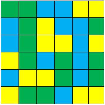
Entropy 2018, 20, 398 5 of 13
3.1. Simulated Landscapes for Validation
Firstly, a set of simulated landscapes is used to evaluate the performances of Hs , Hsc , and IJI.
The fundamental idea behind the simulation strategy is to create a series of increasingly configurational
disordered patterns, and then to examine whether these metrics capture the increasing disorder or
not [25]. In order to obtain a sequence of such landscapes, we followed the discussion by [3,34],
Entropy 2018, 20, x 5 of 13
the mixtures of ideal gases in thermodynamics revisited (see Figure 2). The salient characteristic of
gaseous mixtures is that, as [37] noted, during the mixing process, the disorder of the system increases
logarithmically until the system reaches its thermodynamics equilibrium, i.e., the maximum degree
logarithmically until the system reaches its thermodynamics equilibrium, i.e., the maximum degree
of disorder.
of disorder.
Figure 2. A
Figure 2. A schematic
schematic diagram
diagram ofof ideal
ideal gas
gas mixing
mixing in
in aa closed
closed system.
system. (a)(a) Two
Two kinds
kinds of
of ideal
ideal gases
gases are
are
separated
separated by a partition in a container; (b) The partition is removed and the ideal gases begin to
by a partition in a container; (b) The partition is removed and the ideal gases begin to mix
mix
together;
together; (c)
(c) An
An intermediate
intermediate state
state of
of the
the mixture;
mixture; and
and (d)(d) The
The final
final state,
state, equilibrium,
equilibrium, ofof the
the mixture
mixture
(after [34]).
(after [23]).
Similar to
Similar to the
the process
process of of gaseous
gaseous mixtures,
mixtures, aa set set ofof increasingly
increasingly configurational
configurational disordered
disordered
patterns can
patterns canbe begenerated
generated(see (see[34],
[34],andandthe thesimulation
simulationstrategy
strategyisispresented
presentedininAppendix
Appendix B).B). Figure
Figure 3
3 shows twenty-four different landscape configurations at a dimensionality
shows twenty-four different landscape configurations at a dimensionality of 6 × 6 cells with three of 6 × 6 cells with three
classes and the
classes the same
sameproportion
proportionofofeach eachclass.
class. However,
However, there willwill
there be 36!/(12!
be 36!/(12!× 12! ××12!)12! =× 3.3847e
12!) =+
15 unique
3.3847e + 15 configurations that are generated
unique configurations in this simulation
that are generated strategy. We
in this simulation chooseWe
strategy. them for two
choose them main
for
reasons: on the one hand, these simple landscape patterns
two main reasons: on the one hand, these simple landscape patterns show different configurational show different configurational
information;on
information; onthe
the other
other hand, hand, the increasing
the increasing degree degree of disorder
of disorder (or heterogeneity)
(or heterogeneity) would bewould captured be
captured
by by naked
naked eye. eye. ForFigure
For instance, instance, Figurean
3a shows 3aordered
shows an ordered configuration,
configuration, like the
like the “Initial state”“Initial state”
of gaseous
of gaseousand
mixtures, mixtures,
Figure and Figure 3d
3d presents presents manner
a disorder a disorder manner the
of placing of placing
classes the classes
in space in space
that thatto
is similar is
similar
the to the “Intermediate
“Intermediate state” during state” during the
the mixing, andmixing,
Figure 3x and Figurethe
denotes 3xmost
denotes the most
disordered disordered
arrangement
arrangement
of entities, likeofthe entities, like the “Equilibrium
“Equilibrium state”. In summary, state”. Inthese
summary,
simplethese simple are
landscapes landscapes
useful toare useful
address
to address
the questionthe question
that the rolethatplayedthe role played
by space by space
should should bewhen
be considered considered
entropy when
is usedentropy is usedthe
to evaluate to
evaluate
degree of the degree heterogeneity,
landscape of landscape heterogeneity, in the mostways
in the most perspicuous perspicuous ways [31]. aFurthermore,
[31]. Furthermore, statistical testa
statistical test
(regression (regression
analysis) analysis)
is applied is applied
to evaluate thetovalidation
evaluate the validation
of all of all three
three metrics, that ismetrics, that is to
to say, whether
say, whether
their values oftheir values
these of these
different different
landscape landscape configurations
configurations present a valid present a valid trend
logarithmic logarithmic
[37]. Intrend
this
[37]. Inthe
study, thiscoefficient
study, theofcoefficient
determination (R2 ) values (of the
of determination ) values of the model
regression regression modeltoare
are used usedthe
verify to
2 2
verify theof
goodness goodness
fit, and ifofRfit,isand if than
greater is greater than the
a half, then a half, then themodel
regression regression model be
can usually canregarded
usually as be
aregarded as a good fit [34,38].
good fit [34,38].
Theresults
The resultsof ofthree
threemetrics
metrics(i.e.,(i.e.,HHss,, H
Hscsc, and IJI) are shown in FigureFigure 4. 4. The regression
regression analysis
analysis forfor
each metric
each metric isis also presented, including regression equation and the coefficient of determination ((R2).).
of determination
Thevalues
The valuesof ofthreethree
metricsmetrics for different
for these these different
landscape landscape configurations
configurations exhibit a validexhibit a valid
logarithmic
logarithmic
trend over the trend over of
process themixing
process 2
(Rof ismixing
greater( than is agreater than a half, respectively;
half, respectively; Figure 4).
Figure 4). Statistically
Statistically
speaking, speaking,
these these three
three metrics have metrics
the ability have to the ability todifferent
distinguish distinguish different
landscape landscape
patterns, and patterns,
they can
and they canthe
characterize characterize the degree
degree of disorder of disorder
of these patterns. ofHowever,
these patterns. However,
the results the 4results
in Figure in Figure
also indicate that4
Halso indicate
sc and IJI arethat Hsc andtoIJIthe
insensitive are insensitive
variations amongto the variations
these differentamong
patterns; these
for different
example, patterns;
the valuefor of
Hexample,
sc varies the
from value
1.02 of H
(Figure sc varies
3a) to from
1.69 1.02
(Figure (Figure
3x) among3a) to
the 1.69 (Figure
twenty-four 3x) among
increasingly the twenty-four
configurational
increasingly
disordered configurational
patterns; and, the disordered patterns;from
value of IJI changes and,63.09
the value of IJI
to 98.18 forchanges from 63.09
Figure 3a–d, however, to 98.18 for
ranges
Figure 3a–d, however, ranges from 96.51 (Figure 3p) to 100 (Figure 3v,x) for the following twenty
patterns. In order to make a direct comparison, we further normalize the results of these three metrics
with the same range scope from 0 to 100 (see Figure 5). As Figure 5 shows, the normalized results of
IJI are similar among Figure 3d–x (various from 92.95 to 100); and, the relative values of Hsc for Figure
3j–x change from 91.13 to 100, which also show little variations. In total, when compared with the
performance of Hs, these two metrics are overall less sensitive to the changes in landscape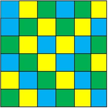
Entropy 2018, 20, 398                                                                                                   6 of 13

from 96.51 (Figure 3p) to 100 (Figure 3v,x) for the following twenty patterns. In order to make a direct
comparison, we further normalize the results of these three metrics with the same range scope from 0
to 100 (see Figure 5). As Figure 5 shows, the normalized results of IJI are similar among Figure 3d–x
(various from 92.95 to 100); and, the relative values of Hsc for Figure 3j–x change from 91.13 to
100, which also show little variations. In total, when compared with the performance of Hs , these
two metrics    are overall less sensitive to the changes in landscape configurations (Figures 64ofand
        Entropy 2018, 20, x                                                                        13
                                                                                                      5).

                           (a)                     (b)                      (c)                      (d)

                           (e)                      (f)                     (g)                      (h)

                           (i)                      (g)                     (k)                      (l)

                           (m)                     (n)                      (o)                      (p)

                           (q)                      (r)                     (s)                      (t)

                           (u)                      (v)                     (w)                      (x)
               Figure 3. Twenty-four different landscape configurations with dimensions 6 × 6, three classes, and the
     Figure 3.   Twenty-four different landscape configurations with dimensions 6 × 6, three classes,
             same proportion of each class. (a) An ordered landscape mosaic, like the “Initial state” of gaseous
     and themixtures;
              same proportion     of each increasingly
                       (b–w) Twenty-two      class. (a) An   ordered landscape
                                                          configurational disorderedmosaic,
                                                                                       patternslike  the “Initial
                                                                                                 similar  to the state”
     of gaseous  mixtures;state”
             “Intermediate (b–w)   Twenty-two
                                 during          increasingly
                                        the mixing; (x) The mostconfigurational
                                                                 disorder manner disordered     patterns
                                                                                 like “Equilibrium   state”.similar to the
     “Intermediate state” during the mixing; (x) The most disorder manner like “Equilibrium state”.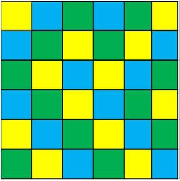
Entropy 2018, 20,
Entropy 2018, 20, 398
x 77 of
of 13
13
Entropy 2018, 20, x 7 of 13
Figure 4. The results
The results of
results of three
of three metrics for twenty-four
three metrics twenty-four increasingly configurational
configurational disordered
Figure
Figure 4.
4. The metrics for
for twenty-four increasingly
increasingly configurational disordered
disordered
landscape
landscape mosaics.
landscape mosaics.
mosaics.
Figure 5. The normalized results of three metrics for twenty-four increasingly configurational
Figure 5.
5. The normalized results of
ofsc’three metrics for
for twenty-four
twenty-four increasingly
increasingly configurational
disordered The
Figure normalized
landscape mosaics. results
Hs’, H three
and IJI’metrics
denote the normalization of metric configurational
Hs, Hsc, and IJI,
disordered
disordered landscape
landscape mosaics. H s’, Hsc ’ and IJI’ denote the normalization of metric Hs, Hsc, and IJI,
respectively. Taking Hmosaics. Hs ’, Hsc ’ and IJI’ denote the normalization of metric Hs , Hsc , and IJI,
s’ for an example, Hs’ = (Hs − Hsmin) × 100/(Hsmax − Hsmin).
respectively. Taking
respectively. TakingHHss’’ for
for an
an example,
example, H Hss’’ =
= (H
(Hss −−HHsmin ) × 100/(Hsmax − Hsmin).
smin ) × 100/(Hsmax − Hsmin ).
3.2. Real-Life Landscapes for Validation
3.2. Real-Life
3.2. Real-Life Landscapes
Landscapes for for Validation
Validation
Secondly, we also use a set of real-life landscapes for the purpose of validation. This set of data
Secondly, we
Secondly, we also
also use
use aa setset ofof real-life
real-life landscapes
landscapes for for the
the purpose
purpose of of validation.
validation. This
This set
set of
of data
data
contains three pairs of different landscape types, including urban, forest, and agriculture landscapes,
contains
contains three pairs of different landscape types, including urban, forest, and agriculture landscapes,
as Figurethree pairsIn
6 shows. of each
differentpair,landscape
the left one, types, including
in fact, urban,offorest,
is a portion and map
land-use agriculture
of Chinalandscapes,
for 2015,
as Figure
as Figure 66 shows.
shows. In In each
each pair,
pair, the left
the left one,
one, in in fact,
fact, is
is aa portion
portion of of land-use
land-use mapmap of
of China
China for
for 2015,
2015,
which are provided by Resource Data Center of Chinese Academy of Sciences (http://www.resdc.cn).
which
which are provided
are provided by Resource Data Center of Chinese Academy of Sciences (http://www.resdc.cn).
This land-use mapby Resource
contains sixData Center classes,
different of Chinese Academy
including of Sciences
forest, water (http://www.resdc.cn).
bodies, built-up area,
This land-use
This land-usemap map contains
contains six six different
different classes,classes,
includingincluding
forest, forest,bodies,
water water built-up
bodies, area,
built-up area,
grassland,
grassland, arable land, and unused land, with a spatial resolution of 1000 m.
grassland,
arableTheland, arable land,
and unused and unused
land,landscape land,
with a spatial with a spatial resolution of 1000 m.
dimension of each type resolution
is 70 × 70, of and1000them. main features of them are shown in
The dimension
The dimension of of each
each landscape
landscape type
type isis7070 ××70,70, andand thethemain
main features
featuresof of
them
them areare
shown in
Table 1. The right landscapes in these pairs are randomly reorganized from the left ones. Thus,shown
when
Table
in 1. The
Table 1. with right
The right landscapes
landscapes in these pairs
in these are randomly reorganized from the left ones. ones. when
Thus,
compared the left landscape type pairs
in each arepair,
randomly the rightreorganized
one has from the left
the same Thus,
compositional
compared
when comparedwith with
the left landscape typetype in each pair, thetheright
rightone
onehas the same
same compositional
information, however,the left landscape
at least by visual observation, in each pair,
is more disordered. has
Thethe
results ofcompositional
three metrics
information,
information, however,
however, at
at least
least by
by visual
visual observation,
observation, is
is more
more disordered.
disordered. The
The results
results of three
of three metrics
metrics
regarding to these landscapes are shown in Table 2.
regarding
regarding to these landscapes are shown in Table 2.
It cantobetheseseenlandscapes
from Table are2 shown
that three in Table 2.
entropy-related metrics can distinguish these different
It
It can
can be
be seen
seen from
from Table
Table 22 that
that three
three entropy-related
entropy-related metrics can
metrics can distinguish
distinguish these
these different
different
landscape patterns, and only Hsc and Hs capture the trend of the configurational disorder of
landscape
landscape patterns, and only H sc and Hs capture the trend of the configurational disorder of
landscapespatterns,
in each pair and only (Figure Hsc6;and Table Hs 2).capture
However,the trendHsc isof less
the sensitive
configurational
to the disorder
changes of in
landscapes
landscapes in each
in each pair
pairvalues(Figure
(Figure 6; Table
6; Table 2). However, H sc is less sensitive to the changes in
configurations, and its among these2).different
However, patternsHsc are is less sensitive
similar to the2).changes
(see Table IJI fails in
to
configurations, and
configurations, and itsits values
values among among these these different patterns patterns are are similar
similar (see
(see Table
Table 2).2). IJI
IJI fails
fails to
to
depict the degree of configurational disorderdifferent
of the last two pairs (Figure 6b1,b2,c1,c2, respectively).
depict
depict the degree of configurational disorder of the last two pairs (Figure 6b1,b2,c1,c2, respectively).
Only Hthe degree of configurational disorder of the last two pairs (Figure 6b1,b2,c1,c2, respectively).
s can distinguish these different patterns effectively and capture the configurational disorder
Only Hs can distinguish these different patterns effectively and capture the configurational disorder
information sensitively.
information sensitively.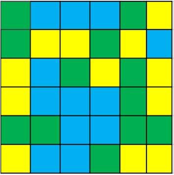
Entropy 2018, 20, 398 8 of 13
Only Hs can distinguish these different patterns effectively and capture the configurational disorder
Entropy 2018, 20,
information x
sensitively. 8 of 13
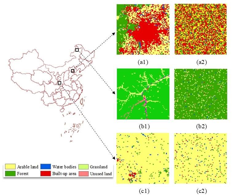
Figure6.6.Three
Figure Three pairs
pairs of different
of different real-life
real-life landscape
landscape types.
types. (a1) Urban(a1)landscape;
Urban landscape;
(b1) Forest(b1) Forest
landscape;
landscape;
and and (c1) Agriculture
(c1) Agriculture landscape. landscape.
The right one The in
right one
each in each
pair pair is randomly
is randomly reorganizedreorganized
from thefrom
left
the left landscape
landscape type, respectively.
type, respectively. Their mainTheir main are
features features
shown areinshown
Table 1.in Table 1.
Table 1. Main features of three different landscape types.
Table 1. Main features of three different landscape types.
Landscapes Latitude Extent Longitude Extent Description
Urban landscape 47.1% built-up area, 29.7% arable land, 19.0% forest
38°50′54″–39°28′04″ 115°47′08″–116°36′54″
(a1) Landscapes Latitude Extent Longitude Extent
land, 1.8% grassland, and Description
2.4% water bodies
89.2% 47.1%
forest land,built-up
0.5% area, 29.7%
arable land, arable land,
7.6% grassland,
Forest Urban
landscape
landscape (a1) 38◦ 500 54”–39◦ 280 04” 115◦ 470 08”–116◦ 360 54” 19.0% forest land, 1.8% grassland, and
51°06′38″–51°43′48″ 121°59′48″–122°49′34″ 0.7% water bodies, 0.2% built-up area, and 1.8%
(b1) 2.4% water bodies
unused land
89.2% forest land, 0.5% arable land,
Agriculture 51◦ 060 38”–51105°44′53″–106°34′39″
Forest landscape38°50′54″–39°37′04″
(b1) ◦ 430 48” 93.2% arable7.6%
121◦ 590 48”–122◦ 490 34”
land, 3.3% forest land, 1.6% built-up
grassland, 0.7% water bodies, 0.2%
landscape (c1) area, 0.5% grassland, 1.4%
built-up area, andwater bodies land
1.8% unused
93.2% arable land, 3.3% forest land,
Agriculture landscape ◦ 0 ◦ 0 ◦ 0 ◦ 0
Table(c1)
2. The 38 50 54”–39
results 37 04”entropy-related
of three 105 44 53”–106 34 39” of real-life
metrics 1.6% built-up area, 0.5% grassland, 1.4%
landscapes.
water bodies
Metrics a1 a2 b1 b2 c1 c2
Table 2. The
Hscresults 1.43
of three entropy-related
1.75 0.53 metrics
0.65 of 0.42
real-life landscapes.
0.47
IJI 62.06 66.18 42.21 39.79 51.91 47.83
Metrics Ha1s 43.43a2 629.34 b16.98 54.93 b2 3.05 c134.07 c2
Note: Hsc, H spatial
sc 1.43 proposed
entropy 1.75 0.53 [21]; IJI,
by Claramunt 0.65 0.42 and juxtaposition
interspersion 0.47 index
IJI 62.06 66.18 42.21 39.79 51.91
proposed by McGarigal and Marks [32]; Hs, the new entropy index proposed in this study. The base 47.83
Hs 43.43 629.34 6.98 54.93 3.05 34.07
of logarithmic in computing each metric is set as 2 in this research, although other bases such as 10
Note: Hsc , spatial entropy proposed by Claramunt [21]; IJI, interspersion and juxtaposition index proposed by
and e are available. The detailed descriptions of these real-life landscapes are shown in Figure 6 and
McGarigal and Marks [32]; Hs , the new entropy index proposed in this study. The base of logarithmic in computing
Table
each 1. is set as 2 in this research, although other bases such as 10 and e are available. The detailed descriptions
metric
of these real-life landscapes are shown in Figure 6 and Table 1.
4. Discussion
Characterizing and distinguishing different landscape patterns have long been the primary
concerns of spatial analysis in landscape ecology. In this study, a new form of spatial entropy (Hs)
has been developed to distinguish and to characterize different landscape configurations. Hs is an
entropy-related index that is based on Shannon entropy, and models proximity as the key factor that
Entropy 2018, 20, 398                                                                                  9 of 13

4. Discussion
      Characterizing and distinguishing different landscape patterns have long been the primary
concerns of spatial analysis in landscape ecology. In this study, a new form of spatial entropy (Hs )
has been developed to distinguish and to characterize different landscape configurations. Hs is
an entropy-related index that is based on Shannon entropy, and models proximity as the key factor
that relates entities in space. Proximity incorporates both the total edge length and distance, and so
it reflects these two important aspects of spatial pattern. In this way, Hs provides a way diversity
(or heterogeneity) should be evaluated in space. Lower values of Hs indicate a landscape pattern
with a weaker degree of spatial heterogeneity, like placing entities in an ordered way in space, i.e.,
entities would be more adjacent to entities of the same class, as TFL describes [29]. In this context,
this new form of spatial entropy is similar to the measure of order and disorder that is proposed by
Bogaert et al. [39]. When compared with the heuristic work by Batty regarding spatial systems analysis
(in [19,21], he developed a derivation of a continuous measure of entropy and applied it to the study
the probability distribution over a progressive distance from a given location), Hs considers the relative
spatial distributions of entities in space.
      Both simulated and real-life landscapes are applied to evaluate the performance of Hs and
similar entropy-related metrics, including Hsc (spatial entropy proposed by Claramunt [23]) and IJI
(interspersion and juxtaposition index that is proposed by McGarigal and Marks [35]). The results of
validation show that all three metrics can distinguish different landscape configurations, and both Hsc
and IJI are overall less sensitive to changes in landscape patterns, and IJI fails to capture the degree
of configurational disorder of these patterns (Figures 3–6; Table 2). However, if a landscape metric
is insensitive to differences in landscape patterns, it is hard (or fails) to detect landscape structural
changes that may be important to understanding ecological processes [40]. The reason why Hsc cannot
effectively distinguish these different landscape patterns lies in that distance is not always the key
factor that relates to entities in space [27,28]. The interspersion and juxtaposition index measures to
which extent patch types (or classes) are interspersed, and is a relative metric that denotes the degree
of interspersion as a percentage of the maximum possible given the total number of patch types [32],
and in fact, it is not a formal entropy metric.
      Since accurately describing and characterizing landscape configuration is a key foundation of
landscape ecology research [8], Hs will help to objectively measure and quantify different landscape
patterns. Furthermore, this new form of spatial entropy may be useful to better explain landscape
patterns, predict ecological process, and understanding the interactions of pattern-process given that
they are all constrained by entropy principles [3,10]. Currently, many scholars concur that landscape
ecologists should pay more attention to the linkages between entropy, complexity theory, and landscape
ecology as a multiple-scale and hierarchical dissipative structures (see [3,12,41]), and we hope that our
new spatial entropy index can contribute to those linkages.
      Another application of Hs , as the experimental results demonstrate, is to measure the degree
of order and disorder of a given spatial pattern at the landscape level. This new entropy index
captures the configurational disorder of both the simulated and real-life landscapes effectively and
sensitively. However, as many scholars’ shrewd observation (e.g., [3,24]), the true thermodynamic
relationship between entropy and landscape configuration still needs to be further investigated, for
instance, the divergent theoretical assumptions between information and thermodynamic entropies,
and the analogy between ideal gases and landscapes. Further research is needed to clarify the true
relationships between spatial patterns and thermodynamic disorder, and at the very least, the Hs
metric that is proposed in this study is highly efficient when compared with similar measures of
landscape configurations.
      It is necessary to note that this research uses Euclidean distance to calculate Hs . However, different
measures of distance (e.g., Manhattan distance, contextual distance, and cognitive distance) can be
considered in the calculation of Hs , which depends on the specific phenomena studied in landscape
ecology [42]. In addition, the simulated landscapes that are presented above are simple landscape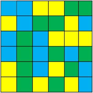
Entropy 2018, 20, 398                                                                                 10 of 13

patterns produced for validation and comparison among the methods in the most perspicuous ways.
The examples (both simulated and real-life ones) that are discussed in this study are regular raster-based
landscapes at a particular level dimensionality, number of classes, and proportionality of each class.
When Hs is applied to more realistic landscapes, higher numbers of classes and proximities make the
interpretation of results more complicated since the definitions of the term entropy and its meanings are
dialectically vague from different perspectives. Also, when Hs is used to irregular and/or vector-based
landscapes, the calculation of proximity would be more complicated, and the complex irregular
patterns (e.g., polygon with holes) would affect the interpretation of results. Thus, this new form of
spatial entropy needs to be further validated on other cases in order to be considered as an efficient
and promising method.

5. Conclusions
     Accurately describing and characterizing landscape patterns are among the core tasks in landscape
ecology research. In this study, we introduce a new form of spatial entropy (Hs ), which is extended
from Shannon entropy, and is derived from the principles of TFL. Hs is an entropy-related index, and it
integrates proximity as the key factor that relates entities in space. It provides a novel way to study
the diversity of spatial structures of landscapes where categories and proximity are relevant to the
analysis. We also tested of the performance of Hs and other similar approaches that are based on both
simulated and real-life landscapes, and found that Hs is more flexible and is sensitive in characterizing
and distinguishing different landscape patterns.
     We believe future research should focus on the following areas: (1) how this new entropy index
would change with dimensionality, number of classes, proportion of each class in the landscape, and
the effects of changing scales on the analysis of landscape patterns; (2) how the spatial entropy of
landscapes that are represented as irregular vector-based patterns can be calculated; (3) the underlying
pattern-process relationships of Hs needs to be further explored, which is a quite important issue in
landscape pattern analysis [43]; and (4) the connections of Hs and other entropy based metrics to true
thermodynamic disorder must be further explored and developed.

Author Contributions: The authors contributed equally in research and experiment design; C.W. performed the
experiment and wrote the paper.
Acknowledgments: The authors greatly appreciate the insightful advice and comments on the manuscript
received from the four reviewers that helped improve the quality of this research. This work was supported by
the Fund of National Natural Science Foundation of China [grant number 41571414].
Conflicts of Interest: The authors declare no conflict of interest.

Appendix A.

(1) Spatial entropy (Hsc , proposed by Claramunt [21])
     Claramunt (2005) introduced the factor of distance and proposed a spatial form entropy based on
information theory. The idea behind his research is to consider the primal role of distance that relates
entities in geo-space. More specifically, he argues that the entropy should augment when distance
between different entities decreases, while the entropy should also augment when the distance between
similar entities increases [27]. Thus, this kind of spatial entropy is defined as follows:

                                                       n  dint
                                            Hsc = − ∑       i
                                                               p log2 pi
                                                            ext i
                                                                                                        (A1)
                                                          d
                                                      i =1 i
Entropy 2018, 20, 398 11 of 13
where dint
i means the average distance between the entities of a given class i (also called intra-distance);
diext denotes the average distance between the entities of a given class i and the entities of the other
classes (also called extra-distance).
Ni Ni
1
dint
i =
Ni ∗ ( Ni − 1) ∑ ∑ d j,k i f Ni > 1, otherwise dint
i =λ (A2)
j=1 k=1
jeCi k 6= j
keCi
Ni N − Ni
1
diext =
Ni ∗ ( N − Ni ) ∑ ∑ d j,k i f Ni 6= N, otherwise diext = λ (A3)
j=1 k=1
jeCi k∈
/ Ci
where Ci denotes the set of entities of a given class i, Ni denotes the number of entities of a given class
i, N the total number of entities, di,j is the distance between two entities i and j, λ is a constant taken
relatively small (such as 0.2 or 0.5-unit length) in order to avoid the “noise” effect of null values in the
calculations of the average distances [21].
Hsc is semi bounded by the interval [0, +∞], and augments when the intra-distance increases, or
the extra-distance decreases [21]. For some given intra- and extra-distance values, Hsc is maximum
when the classes are evenly distributed.
(2) Interspersion and juxtaposition index (IJI, McGarigal and Marks [32])
McGarigal and Marks (1995) introduced the interspersion and juxtaposition index to measure the
extent to which the patch type (or classes) are interspersed (i.e., equally adjacent to each other), and
lower values characterize landscapes in which the patch types are poorly interspersed. This index (IJI)
is computed as follows:
h i
Lik Lik
− ∑in=1 ∑nk=i+1 L ∗ log2 L
IJI = − (100) (A4)
log2 (0.5(n(n − 1)))
where Lik denotes the total length of edge in landscape between patch type (or classes) i and k, L
refers to the total length of edge in landscape excluding background, n refers to number of classes in
the landscape.
IJI increases in value as patch types tend to be more evenly interspersed, and it ranges from 0 to
100 [32]. When all patch types are equally adjacent to all other patch types, IJI reaches its maximum
value (100).
Appendix B.
The simulation strategy of those twenty-four different landscape patterns (Figure 3) is based on
descriptions and discussions in [34], but much simple (only 6 × 6 cells with three classes and the same
proportion of each class are considered). The simulation strategy contains four main steps:
1. set Figure 3a as the “seed” pattern, which is regarded as the initial state of a closed system
(an ordered landscape mosaic).
2. then select three cells from middle to the sides in the “seed” pattern, and exchange the position
of each cell with randomly selected neighboring cell.
3. repeat Step 2 until the pattern is similar to Figure 3x (the most disordered manner like
“Equilibrium state” of gaseous mixtures).
4. then choose twenty-two patterns from the output of Step 2. In this way, we can obtain a set of
increasingly configurational disordered patterns. It should be noted that, the choose of theseEntropy 2018, 20, 398 12 of 13
twenty-two patterns may be affected by subjective factors, however, the most important thing
is that they should present in an increasingly configurational disordered way, which would be
captured by naked eye.
These simulated landscape patterns and related algorithms associated with this research are
available on online at https://pan.baidu.com/s/1jgLF2PBinmtQDyczNFehBA.
References
1. Lausch, A.; Blaschke, T.; Haase, D.; Herzog, F.; Syrbe, R.U.; Tischendorf, L.; Walz, U. Understanding and
quantifying landscape structure—A review on relevant process characteristics, data models and landscape
metrics. Ecol. Model. 2015, 295, 31–41. [CrossRef]
2. O’Neill, R.V.; Krummel, J.R.; Gardner, R.H.; Sugihara, G.; Jackson, B.; Deangelis, D.L.; Milne, B.T.;
Turner, M.G.; Zygmunt, B.; Christensen, S.W. Indices of landscape pattern. Landsc. Ecol. 1988, 1, 153–162.
[CrossRef]
3. Cushman, S.A. Calculating the configurational entropy of a landscape mosaic. Landsc. Ecol. 2016, 31, 481–489.
[CrossRef]
4. Wu, J. Key concepts and research topics in Lands. Ecol. revisited: 30 years after the Allerton Park workshop.
Landsc. Ecol. 2013, 28, 1–11. [CrossRef]
5. Forman, R.T.; Godron, M. Landscapes Ecology Principles and Landscape Function. 1984. Available online:
http://agris.fao.org/agris-search/search.do?recordID=US201301428863 (accessed on 20 May 2018).
6. Li, H.; Reynolds, J.F. A new contagion index to quantify spatial patterns of landscapes. Landsc. Ecol. 1993, 8,
155–162. [CrossRef]
7. Lustig, A.; Stouffer, D.B.; Roigé, M.; Worner, S.P. Towards more predictable and consistent landscape metrics
across spatial scales. Ecol. Indic. 2015, 57, 11–21. [CrossRef]
8. Turner, M.G. The Effect of Pattern on Process. Ann. Rev. Ecol. Syst. 1989, 20, 171–197. [CrossRef]
9. Wu, J. Cross-disciplinarity, and Sustainability Science. Landsc. Ecol. 2006, 21, 1–4. [CrossRef]
10. Cushman, S.A. Thermodynamics in landscape ecology: The importance of integrating measurement and
modeling of landscape entropy. Landsc. Ecol. 2015, 30, 7–10. [CrossRef]
11. Parrott, L. Measuring ecological complexity. Ecol. Indic. 2010, 10, 1069–1076. [CrossRef]
12. Zaccarelli, N.; Li, B.L.; Petrosillo, I.; Zurlini, G. Order and disorder in ecological time-series: Introducing
normalized spectral entropy. Ecol. Indic. 2013, 28, 22–30. [CrossRef]
13. Rodríguez, R.A.; Herrera, A.M.; Quirós, Á.; Fernández-Rodríguez, M.J.; Delgado, J.D.; Jiménez-Rodríguez, A.;
Fernández-Palacios, J.M.; Otto, R.; Escudero, C.G.; Luhrs, T.C. Exploring the spontaneous contribution of
Claude E. Shannon to eco-evolutionary theory. Ecol. Modol. 2016, 327, 57–64. [CrossRef]
14. Shannon, C.E. A mathematical theory of communication. Bell Syst. Tech. J. 1948, 27, 379–423. [CrossRef]
15. Harte, J. Maximum Entropy and Ecology: A Theory of Abundance, Distribution, and Energetics; Oxford University
Press: England, UK, 2011.
16. Macarthur, R. Fluctuations of Animal Populations and a Measure of Community Stability. Ecology 1955, 36,
533–536. [CrossRef]
17. Giliarov, A.M. Information theory in ecology. Comput. Chem. 2001, 25, 393–399.
18. Li, H.; Reynolds, J.F. A Simulation Experiment to Quantify Spatial Heterogeneity in Categorical Maps.
Ecology 1994, 75, 2446–2455. [CrossRef]
19. Batty, M. Spatial entropy. Geogr. Anal. 1974, 6, 1–31. [CrossRef]
20. Wilson, A.G. Entropy in Urban and Regional Modelling; Routledge: Abingdon, UK, 1970.
21. Batty, M. Space, Scale, and Scaling in Entropy Maximizing. Geogr. Anal. 2010, 42, 395–421. [CrossRef]
22. Batty, M.; Morphet, R.; Masucci, P.; Stanilov, K. Entropy, Complexity, and Spatial Information. J. Geogr. Syst.
2014, 16, 363–385. [CrossRef] [PubMed]
23. Claramunt, C. A Spatial Form of Diversity; Springer: Berlin/Heidelberg, Germany, 2005; pp. 218–231.
24. Vranken, I.; Baudry, J.; Aubinet, M.; Visser, M.; Bogaert, J. A review on the use of entropy in Landscape
Ecology: Heterogeneity, unpredictability, scale dependence and their links with thermodynamics.
Landsc. Ecol. 2015, 30, 51–65. [CrossRef]
25. Gao, P.; Zhang, H.; Li, Z. A hierarchy-based solution to calculate the configurational entropy of landscape
gradients. Landsc. Ecol. 2017, 32, 1–14. [CrossRef]Entropy 2018, 20, 398 13 of 13
26. Goodchild, M.F. The Validity and Usefulness of Laws in Geographic Information Science and Geography.
Ann. Assoc. Am. Geogr. 2004, 94, 300–303. [CrossRef]
27. Miller, H.J. Tobler’s First Law and Spatial Analysis. Ann. Assoc. Am. Geogr. 2004, 94, 284–289. [CrossRef]
28. Cao, C.; Li, X.; Yan, J. Geo-spatial Information and Analysis of SARS Spread Trend. J. Remote Sens. 2003, 7,
241–244.
29. Tobler, W.R. A Computer Movie Simulating Urban Growth in the Detroit Region. Ecol. Geogr. 1970, 46,
234–240. [CrossRef]
30. Tobler, W. On the First Law of Geography: A Reply. Ann. Assoc. Am. Geogr. 2004, 94, 304–310. [CrossRef]
31. Claramunt, C. Towards a Spatio-Temporal Form of Entropy; Springer: Berli/Heidelberg, Germany, 2012;
pp. 221–230.
32. McGarigal, K.; Cushman, S.A.; Ene, E. FRAGSTATS v4: Spatial Pattern Analysis Program for Categorical
and Continuous Maps. 2015. Available online: http://www.umass.edu/landeco/research/fragstats/
documents/fragstats.help.4.2.pdf (accessed on 2 November 2016).
33. Wei, X.; Xiao, Z.; Li, Q.; Li, P.; Xiang, C. Evaluating the effectiveness of landscape configuration metrics from
landscape composition metrics. Landsc. Ecol. Eng. 2017, 13, 169–181. [CrossRef]
34. Gao, P.C.; Li, Z.L.; Zhang, H. Thermodynamics-Based Evaluation of Various Improved Shannon Entropies
for Configurational Information of Gray-Level Images. Entropy 2018, 20, 19. [CrossRef]
35. McGarigal, K.; Marks, B.J. Spatial Pattern Analysis Program for Quantifying Landscape Structure. 1995.
Available online: https://pdfs.semanticscholar.org/1cca/4307c5cb70ed82b72b9714bde5d0d32aa646.pdf
(accessed on 18 May 2018).
36. Matlab. MATLAB and Statistics Toolbox Release 2017b; The MathWorks, Inc.: Natick, MA, USA, 2017;
Available online: http://www.mathworks.com/help/matlab/index.html (accessed on 20 May 2018).
37. Vonk, M.E.; Tripodi, T.; Epstein, I. Research Techniques for Clinical Social Workers; Columbia University Press:
New York, NY, USA, 2007.
38. Finkelstein, M.O. Basic Concepts of Probability and Statistics in the Law; Springer: New York, NY, USA, 2009.
39. Bogaert, J.; Farina, A.; Ceulemans, R. Entropy increase of fragmented habitats: A sign of human impact?
Ecol. Indic. 2005, 5, 207–212. [CrossRef]
40. Shao, G.; Wu, J. On the accuracy of landscape pattern analysis using remote sensing data. Landsc. Ecol. 2008,
23, 505–511. [CrossRef]
41. Li, B.L. Why is the holistic approach becoming so important in landscape ecology? Landsc. Urban Plan. 2000,
15, 27–41. [CrossRef]
42. Keersmaecker, W.; Lhermitte, S.; Honnay, O.; Farifteh, J.; Somers, B.; Coppin, P. How to measure ecosystem
stability? An evaluation of the reliability of stability metrics based on remote sensing time series across the
major global ecosystems. Glob. Chang. Biol. 2014, 20, 21–49. [CrossRef] [PubMed]
43. Li, H.; Wu, J. Use and misuse of landscape indices. Landsc. Ecol. 2004, 19, 389–399. [CrossRef]
© 2018 by the authors. Licensee MDPI, Basel, Switzerland. This article is an open access
article distributed under the terms and conditions of the Creative Commons Attribution
(CC BY) license (http://creativecommons.org/licenses/by/4.0/).You can also read