Computers and Mathematics with Applications - Yan ...
←
→
Page content transcription
If your browser does not render page correctly, please read the page content below
Computers and Mathematics with Applications 81 (2021) 532–546

                                                   Contents lists available at ScienceDirect

                           Computers and Mathematics with Applications
                                            journal homepage: www.elsevier.com/locate/camwa

A moving-domain CFD solver in FEniCS with applications to
tidal turbine simulations in turbulent flows
                                      ∗
Qiming Zhu, Jinhui Yan
Department of Civil and Environmental Engineering, University of Illinois at Urbana–Champaign, Urbana, IL, 61801, USA

article             info                           a b s t r a c t

Article history:                                   A moving-domain computational fluid dynamics (CFD) solver is designed by deploying
Available online 12 August 2019                    the Arbitrary Lagrangian Eulerian Variational Multi-scale Formulation (ALE-VMS) en-
                                                   hanced with weak enforcement of essential boundary conditions (weak BC) into the
Keywords:
                                                   open-source finite element automation software FEniCS. The mathematical formulation
Tidal energy
FEniCS                                             of ALE-VMS, which is working as a Large Eddy Simulation (LES) model for turbulent
ALE-VMS                                            flows, and weak BC, which is acting as a wall model, are presented with the imple-
Weak BC                                            mentation details in FEniCS. To validate the CFD solver, simulations of flow past a
                                                   stationary sphere are performed with moving meshes first. Refinement study shows the
                                                   results quickly converge to the reference results with fixed grids. Then, the solver is
                                                   utilized to simulate a tidal turbine rotor with uniform and turbulent inflow conditions.
                                                   Good agreement is achieved between the computational results and experimental
                                                   measurements in terms of thrust and power coefficients for the uniform inflow case. The
                                                   effect of the inflow turbulence intensity on the tidal turbine performance is quantified.
                                                                                                                   Published by Elsevier Ltd.

1. Introduction

    Tidal energy is one of the most promising renewable energy sources in the United States. In the research and develop-
ment of tidal energy, the computational fluid dynamics (CFD) simulation is a powerful tool to quantify the hydrodynamic
loads and predict the performance of tidal turbine design in turbulent flows. Accurate numerical simulations of tidal
turbines are very challenging due to the complexity of turbine geometry and high Reynolds (Re) number turbulent flows
around it. Although a lot of numerical simulations of tidal turbines can be found in the literature, most of them utilize
lumped turbine geometry and reduced order fluid model [1]. The number of high fidelity CFD tools that can enable 3D,
time-dependent, full scale, and full-geometry resolved numerical simulations is still quite few.
    Developing high-fidelity CFD codes for specific applications can be labor-intensive and time-consuming. On the other
hand, open-source simulation platforms can minimize the users’ need for implementation and therefore greatly improve
the efficiency of the analysis workflow. Among many open-source CFD packages, OpenFOAM, which makes use of the
finite volume method, is widely used. The applications of OpenFOAM to wind energy, fluidization, biomass pyrolysis,
and additive manufacturing can be found in [2–7]. However, modification of the OpenFOAM code to generate a specific
application code still requires a relatively deep understanding of numerical analysis of the users. In order to develop
a moving-domain CFD solver that is easy to be modified and upgraded, in this paper, we deploy Arbitrary Lagrangian
Eulerian Variational Multi-scale (ALE-VMS) method enhanced with Weak Enforcement of Essential Boundary Conditions

 ∗ Corresponding author.
    E-mail address: yjh@illinois.edu (J. Yan).

https://doi.org/10.1016/j.camwa.2019.07.034
0898-1221/Published by Elsevier Ltd.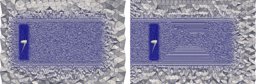
Q. Zhu and J. Yan / Computers and Mathematics with Applications 81 (2021) 532–546         533

in FEniCS, which is an open-source finite element automation software. On the one hand, FEniCS is a convenient open-
source package that is able to automatically transform a variational formulation to a high performance C++ finite element
code [8] in an effective way. FEniCS has many interfaces with many popular numerical analysis packages such as
PETSc [9] and Slepc [10]. It is extremely efficient to implement the finite element code for a partial differential equation
(PDE) as long as the corresponding variational formulation is provided [8]. On the other hand, moving-domain fluid
mechanics formulations, such as ALE-VMS and Space-Time VMS (ST-VMS), are powerful boundary-fitted techniques to
solve engineering problems with moving-domains and moving interfaces [11–19]. In this paper, the solver makes use of
ALE-VMS. ALE-VMS is extended from Residual-based Variational Multi-scale Formulation (RBVMS), which was originally
proposed in [20] to simulate high Re number turbulent flows. Weak enforcement of essential boundary conditions (weak
BC) originally proposed in [21] is aimed to provide a wall model to relax the resolution of boundary layers, which are
impossible to be fully resolved in large spatial engineering CFD calculation. Weak BC is widely used for many CFD and
fluid–structure interaction (FSI) problems, such as wind turbines [22–28]. Instead of strongly setting fluid velocity equal to
the structural velocity, weak BC allows the fluid slightly slip on the fluid–structure interface without losing the accuracy
of fluid load prediction. A comparison of strong BC and weak BC in wind turbine simulations can be found in [29]. It shows
weak BC has superior performance over strong BC with a relatively coarse resolution of the blade boundary layers. Since
their conception, these moving-domain fluid mechanics formulation enhanced weak BC are widely applied to simulate
challenging fundamental flow physics problems [30–37] as well as real-world engineering problems, including renewable
energy [25,26], biomechanics [38–42], vehicle engineering [43,44], gas turbines [45,46], water sport equipment [47,48],
bridge engineering [49], and military applications [50,51,51,52]. Thus, we believe implementing ALE-VMS with weak BC
in FEniCS will not only present an excellent demonstration of the advantages of both the numerical formulation and
FEniCS but also provides a starting point for developing advanced moving-domain CFD code that can be widely used for
fundamental and practical applications.
    The paper is structured as follows. In Section 2, the governing equations and the ALE-VMS with weak BC are presented.
The implementation in FEniCS is also described in detail such that the readers can easily duplicate the solver in FEniCS.
In Section 3, two problems are solved by using the proposed solver. First, flow past a stationary sphere at Re = 400
is simulated with rotating meshes. Drag coefficient Cd is compared with DNS result. Refinement study is performed
to validate the proposed solver. Then tidal turbine simulations using uniform and turbulent inflow conditions are
presented. The method of inflow turbulence generation is presented first. The thrust and power coefficients of the uniform
inflow condition are compared with experimental measurements. Good agreement is achieved. The effect of the inflow
turbulence intensity on the coefficients is quantified as well. In Section 4, conclusions are drawn.

2. Numerical formulation

2.1. Governing equations and semi-discrete formulation

   The Navier–Stokes equations of incompressible flows on moving-domains with ALE technique are defined as
       ∂ u ⏐⏐
            ⏐
               + u − û · ∇x u = ∇x · 2ν∇xs u − pI + f
                (      )             (            )
                                                                                                                           (1)
       ∂ t ⏐x̂
       ∇x · u = 0                                                                                                          (2)

where u, û, p, and f are the fluid velocity, fluid domain velocity, pressure and body force respectively. ν is the kinematic
viscosity, given by ν = µ/ρ , where µ is the dynamical viscosity, and ρ is the density. ∇xs is the symmetric part of the
gradient operator. I is the identity matrix. Note that, in the ALE formulation, the time derivatives are taken with respect
to a referential fluid domain held fixed, while the space derivatives are taken with respect to the current fluid domain.
In ALE, fluid velocity u and fluid domain velocity û are independent, which allows significant flexibility for choosing
appropriate mesh moving schemes.
   To solve Eq. (1) and Eq. (2), the Arbitrary Lagrangian Eulerian Variational Multi-scale formulation (ALE-VMS) is adopted.
ALE-VMS is an extension of the Residual-based Variational Multi-scale Formulation (RBVMS) to simulate turbulent flows
on moving-domains. For the completeness, the semi-discrete formulation of ALE-VMS is presented as follows. Let Ωt
denote the moving fluid domain, Γt denote its boundary, V h denote the discrete trial function space for the velocity
and pressure {uh , ph }, W h denote the discrete testing function space for the linear momentum, continuity equations, the
operator (X1 , X2 )A denote the L2 -inner product of X1 and X2 over the domain A, taken element-wise. With these notations,
the semi-discrete formulation of ALE-VMS reads:
       Find {uh , ph } ∈ Vh s.t. ∀ {vh , qh } ∈ Wh :
                                                                                                                           (3)
       BALE −VMS ({vh , qh }, {uh , ph }) = F ALE −VMS ({vh , qh })

where F ALE −VMS ({vh , qh }) is given as

       F ALE −VMS ({vh , qh }) = (vh , f)Ωt + (vh , h)Γ h                                                                  (4)
                                                        t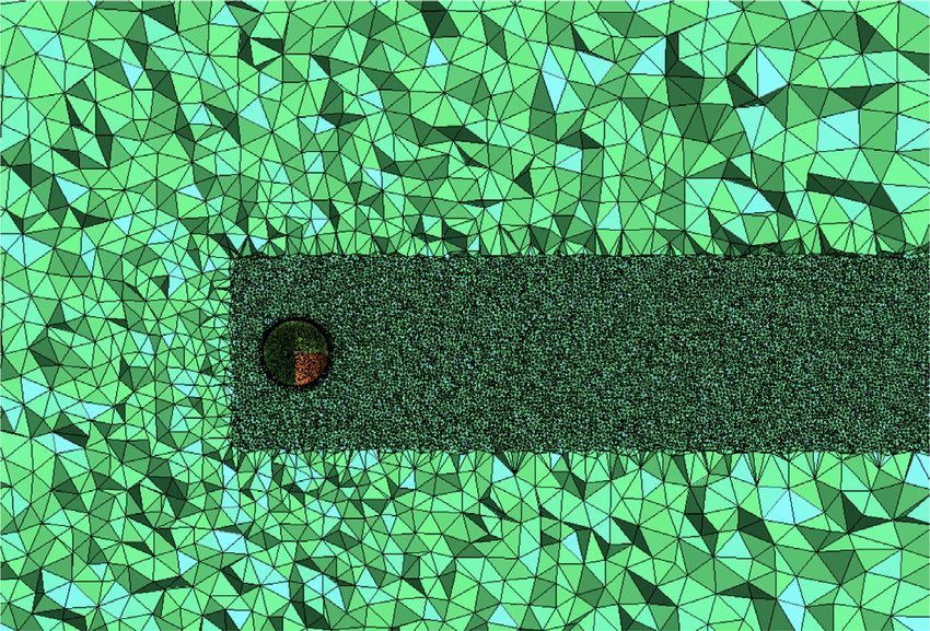
534                                Q. Zhu and J. Yan / Computers and Mathematics with Applications 81 (2021) 532–546

where h is the applied traction on the natural boundary Γth . In Eq. (3), BALE −VMS ({vh , qh }, {uh , ph }) = BG ({vh , qh }, {uh , ph }) +
BFine ({vh , qh }, {uh , ph }), where BG and BFine are the standard Galerkin formulation and the fine-scale terms derived from
ALE-VMS approach, which are given as
                                          ∂ uh ⏐⏐
                                                ⏐
       B ({vh , qh }, {uh , ph }) = (vh ,
         G
                                                   + (uh − ûh ) · ∇x uh )Ωt + (∇xs vh , 2ν∇xs uh − ph I)Ωt
                                           ∂ t ⏐x̂                                                                                      (5)
                                  + (qh , ∇x · uh )Ωt
and
       BFine ({vh , qh }, {uh , ph }) = (uh − ûh ) · ∇x uh , τM rM (uh , ph )          + (∇x · vh , τC rC (uh ))Ωt
                                         (                                     )
                                                                                   Ωt
                                      + (∇x qh , τM rM (uh , ph ))Ωt − (vh · (∇x uh )T , τM rM (uh , ph ))Ωt                            (6)
                                      − (∇x vh , τM rM (uh , ph ) ⊗ τM rM (uh , ph ))Ωt
where rM (uh , ph ) and rC (uh ) are the residuals of strong form momentum and continuity equations, given as
                              ∂ uh ⏐⏐
                                    ⏐
       rM (uh , ph )        =          + (uh − ûh ) · ∇x uh − f − ∇x · (2ν∇xs uh − ph I)
                               ∂ t ⏐x̂                                                                                                  (7)
       rC (uh )             = ∇x · uh
τM and τC are the corresponding stabilization parameters, defined as
                                        )−1/2
                        4∥uh ∥2   16ν 2
               (
                  4
      τM =            +         +
                 ∆t 2     h2       h4
                                                                                                                                        (8)
                       h2
       τC     =
                  12τM
where h is the characteristic element length, h is set to minimum edge length of tetrahedron element in this paper.
The stabilization parameters utilized in this paper are based on the Streamline-Upwind/Petrov–Galerkin (SUPG) [53] and
Pressure Stabilization Petrov–Galerkin (PSPG) [54]. Other possible definitions and more discussions on the stabilization
parameters can be found in [53–57].
    Fully resolving of viscous turbulent boundary layers of large spatial scale CFD simulations with high Re number
turbulent flows is extremely computationally expensive. To relax the resolution requirement of boundary layers without
sacrificing the accuracy of fluid loading prediction, the ALE-VMS formulation is upgraded with the weak enforcement of
essential boundary conditions (weak BC), which was originally developed in [21] and has been successfully applied to
wind turbine simulations [22–27]. For that, the following terms acting on the essential boundary ΓtS are added to the
left-hand side of Eq. (3).

       − (vh , 2ν∇xs (uh ) · n − ph n)Γ S − (2ν∇xs (vh ) · n + qh n, uh − g)Γ S                                                         (9)
                                                 t                                       t

       − (vh · (uh − ûh ) · n, uh − g)Γ S − + (τtan (vh − (vh · n)n), (uh − g) − ((uh − g) · n)n)Γ S
                                                     t                                                                t

       + (τnor vh · n, (uh − g) · n)Γ S
                                             t

where g is the prescribed velocity, the inflow part is defined as ΓtS − = {x | (uh − ûh ) · n < 0 , ∀x ⊂ ΓtS }, τtan and τnor are
small penalty parameters chosen for the balance of accuracy and numerical stability, which, in general, can be different for
the tangential and normal directions. In this paper, the no-slip boundary condition is used on the fluid–structure interface,
and the same penalty parameter is adopted, namely,
                            4ν
       τtan = τnor =                                                                                                                   (10)
                            h
    Other key numerical details are summarized as follows. Generalized-α is adopted for time integration. A two-stage
predictor–multicorrector algorithm based on Newton’s method is used to solve the nonlinear equations. The resulting
linear systems are solved by the linear solver in PETSc [9] embedded in FEniCS, which will be briefly described below. All
the simulations make use of linear elements and are performed in a parallel setting by using the Bluewater supercomputer
at the University of Illinois at Urbana–Champaign.

2.2. FEniCS implementation

   FEniCS is an open-source finite element simulation platform to address this issue. The idea of FEniCS is to enable
automated solutions of partial differential equations (PDEs) based on their variational formulations. In FEniCS, the special
purpose code can be generated automatically from a high-level description of the differential operator by combining
reusable components of finite element algorithms, such as assembling and linear solvers, with automated code generation
for the computation of the discrete operators [8]. These concepts are illustrated in Fig. 1.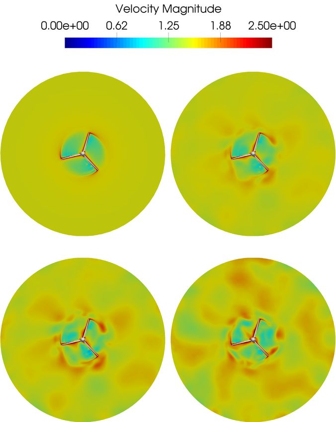
Q. Zhu and J. Yan / Computers and Mathematics with Applications 81 (2021) 532–546             535

                                                       Fig. 1. Concept of FEniCS.

                                                Fig. 2. Trial and testing function space.

                                                      Fig. 3. Variable definitions.

    FEniCS is composed of many core components that include UFL (Unified Form Language) [58], FIAT (Finite element
Automatic Tabulator), FFC (FEniCS Form Compiler) [59], UFC (Unified Form-assembly Code) [60], Instant [61] and
DOLFIN [62]. UFL is a special language for implementing the variational formulation. FFC is a compiler that transforms
the UFL language into the corresponding C++ interface code (UFC). Finite element basis functions and the corresponding
quadrature rules are defined in FIAT. The data structures, assembly routine, linear solvers are defined in DOLFIN. To provide
some details of the CFD solver, the definitions of basis function spaces, variables, residuals of strong form equations,
stabilization parameters, and variational formulation of ALE-VMS based on UFL in the FEniCS code are given step by step
in the following.
    Fig. 2 shows the definition of the trial and testing function space utilized in the FEniCS code. ALE-VMS allows using
equal-order basis functions for both velocity and pressure fields. Thus, tetrahedron elements are used here for both
pressure and velocity fields, although it is easy to change to high order basis functions in FEniCS.
    Fig. 3 shows the variable definitions. du1 and p1 are the acceleration and pressure on n + 1 step, which need to be
solved. du0 and u0 are the acceleration and velocity on n step, which are knowns. ur is the mesh velocity, fx is external
body force, k is the number of time step, idt is the reciprocal of time step, v u is kinematic viscosity and n is face normal
vector. h is the element length.
    Fig. 4 shows the definitions of the stabilization parameters and penalty parameters in Eqs. (8) and (10).
    Fig. 5 shows the quadrature rule in the code. Four quadrature points are used for the volume integration in this paper.
    Fig. 6 shows some predefined functions in the variational formulation. epsilon(u) is the symmetric part of the velocity
gradient tensor, sigma(u, p) is the stress tensor, and Identity is the identity matrix.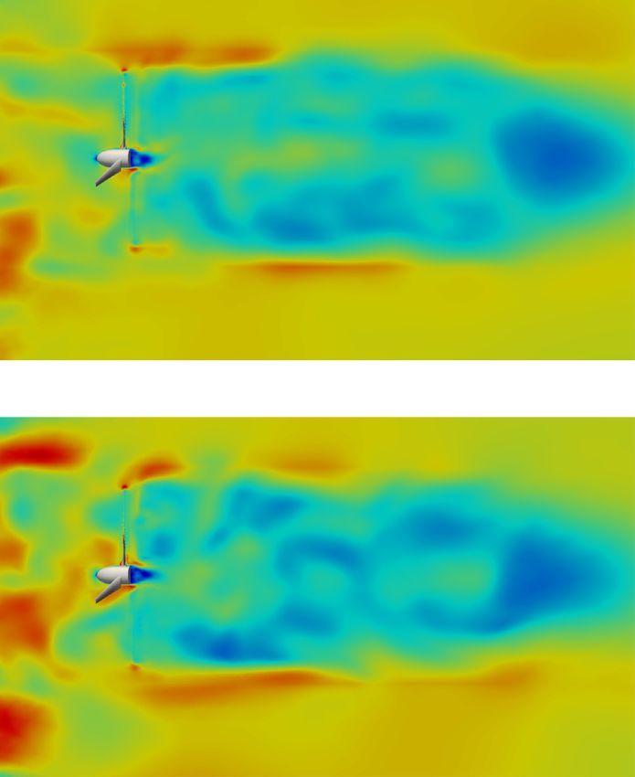
536                        Q. Zhu and J. Yan / Computers and Mathematics with Applications 81 (2021) 532–546

                                             Fig. 4. Stabilization and penalty parameters.

                                                 Fig. 5. Definition of quadrature rule.

                                                     Fig. 6. Predefined functions.

                                       Fig. 7. Residuals of momentum and continuity equations.

                                                   Fig. 8. Galerkin part in the code.

   Fig. 7 shows the definitions of the residuals of momentum and continuity equations in the code. nabla_grad(u) denote
the velocity gradient and nabla_div (T) denote the divergence of a tensor T. Please note that Laplacian operator in the
residual of momentum equations is zero since linear basis functions are used (a L2 projection could be used to approximate
the Laplace operator [63].)
   Figs. 8 and 9 show the Galerkin formulation, the entire ALE-VMS formulation, respectively. Fig. 10 shows the FEniCSs
code after weak BC is added. As can be seen, it is natural to define the complex functions and their derivative of the
variational formulation in a very convenient way by using the powerful UFL language in FEniCS, which will automatically
transfer the variational formulation into a high performance C++ finite element code.

3. Numerical simulations

   To demonstrate the capability of the solver, flow past a stationary sphere at laminar flow region is first simulated with
rotating meshes to validate the CFD solver in FEniCS. Then, the solver is used to simulate a tidal turbine rotor with both
uniform inflow and turbulent inflow conditions with different turbulence intensities.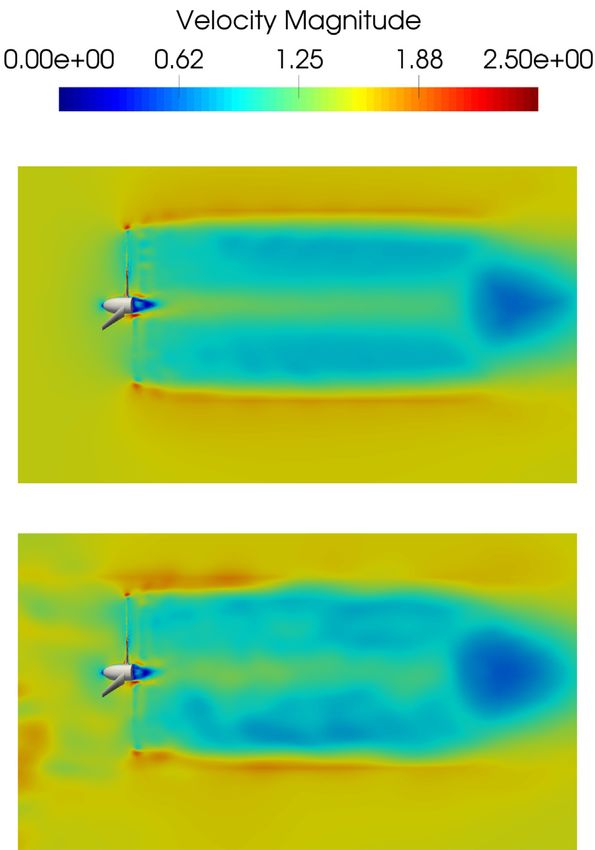
Q. Zhu and J. Yan / Computers and Mathematics with Applications 81 (2021) 532–546               537

                                                     Fig. 9. ALE-VMS part in the code.

                                                     Fig. 10. Weak BC part in the code.

                                      Table 1
                                      Number of nodes and elements.
                                       Mesh                                    Num. of elements
                                       Coarse                                  546,468
                                       Medium                                  1,322,317
                                       Fine                                    4,233,195

                                      Table 2
                                      Element lengths of the meshes.
                                       Mesh              Sphere        Refined box         Out box
                                       Coarse            0.004         0.020               0.20
                                       Medium            0.003         0.015               0.15
                                       Fine              0.002         0.010               0.10

                               Table 3
                               Drag coefficients.
                                            Coarse            Medium           Fine               Reference
                                Cd          0.581             0.585            0.588              0.590 [64]

3.1. Flow past a sphere with rotating meshes

    Flow past a stationary sphere at Re = 400 [64] is widely utilized for validation purpose for CFD solvers, due to rich
experimental or computational results in the literature. Although this problem is typically solved with fixed meshes,
to demonstrate the moving-domain features of the ALE-VMS, a fixed angular speed of 5 rad/s is prescribed for the fluid
domain. Considering the fluid velocity is totally independent of the fluid domain velocity, the ALE-VMS simulations should
produce the same results as that with fixed meshes for this problem.
    Fig. 11 shows the mesh of the problem. The diameter of the sphere is 0.2. The values of inflow velocity and kinematic
viscosity are chosen such that the desired Re number is achieved. A refined region is built around the sphere to resolve
flow physics better. Refinement study of the element length is performed. The mesh statistics of the three meshes is
summarized in Tables 1 and 2. Since the Re is low, strong no-slip boundary condition is used on the sphere.
    Fig. 12 shows the vortex structure based on Q -criterion, which is defined as Q = 12 (|O|2 − |S|2 ), where S =
1
2
  (∇ u + (∇ u)T ) is the rate of strain tensor and O = 12 (∇ u − (∇ u)T ). Classis Hairpin vortex [65] can be observed. Table 3
provides the comparison of the predicted averaged drag coefficients and the reference result from [64]. As the mesh size
is refined, drag coefficients predicted by the present approach gradually converge to the reference result.

3.2. Tidal turbine simulations with uniform and turbulent inflow conditions

    In this section, the FEniCS CFD solver is utilized to simulate a three-blade tidal turbine rotor with both uniform and
turbulent inflow conditions. The tidal turbine rotor has a pitch angle of 20◦ and a radius of 0.4 m, obtained from [66]. This
turbine design is also used in our previous free-surface simulations [67]. For more details about the turbine, the readers
are referred to [66]. The front side and back side of the turbine are shown in Fig. 13. The operation condition is set as
follows: the rotation rate is 28.125 rad/s, and inflow velocity is 1.5 m/s, which defines the tip speed ratio (TSR) as 7.5.
Fig. 14 shows the computational domain, which is a cylinder rotating with the same rotational speed of the rotor during
the simulations. A refined inner cylinder is designed to capture the wake better. As shown in Fig. 15, this refined cylinder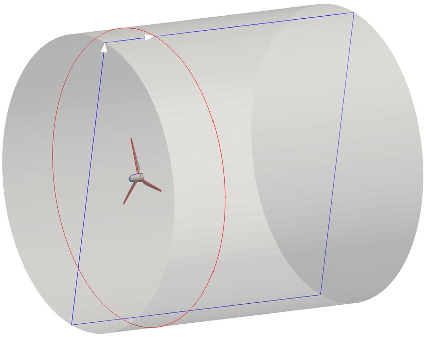
538                              Q. Zhu and J. Yan / Computers and Mathematics with Applications 81 (2021) 532–546

                                                           Fig. 11. Mesh of flow past sphere (fine mesh).

                                                     Fig. 12. Vortex structure colored by velocity magnitude.

                                          Table 4
                                          Number of nodes and elements.
                                          Cases                       Num. of nodes               Num. of elements
                                          Uniform                     989,118                     5,853,413
                                          Turbulent                   1,080,942                   6,398,312

                                                  Table 5
                                                  Element length for different regions (m)
                                                     Outer cylinder           Refined region          Rotor
                                                     0.4                      0.02                    0.0005

is extended to the inlet for the turbulent mesh to capture the inflow turbulence. The mesh statistics are summarized in
Tables 4 and 5. The boundary conditions are set as follows. Strong boundary condition is utilized for the inlet. Traction
free boundary is used for the side wall of cylinder. Zero pressure is used for the outlet. Weak enforcement of no-slip
boundary condition is used for the fluid–turbine interface. Simulation is performed until the flow reach to turbulence
statistical stationary stage with a constant time step ∆t = 10−4 s.

3.2.1. Inflow turbulence generation
   To generate the inflow turbulence for tidal turbine simulation, an offline code using synthetic eddy method (SEM) [68]
is utilized. SEM makes use of Lagrangian treatment for the vortices and assumes the velocity at one point is the
combination of the influence from all the neighboring vortices. The vortices are generated randomly and move with
mean stream velocity. In SEM, the velocity fluctuation u′i (x) that is influenced by N vortices is defined by the following
equation:
                   N
                                              x − xk
                                          (            )
                 1 ∑
      ui (x) = √
        ′
                                σ
                             aij jk fσk                                                                                      (11)
                   N                            sk
                       k=1

where xk is the position of the kth vortex, sk is empirical length scale of the vortex and fσk is the shape function. σjk contains
randomly assigned eddy intensities which obey a Gaussian distribution with zero mean value and a standard deviation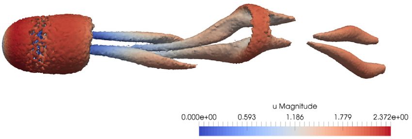
Q. Zhu and J. Yan / Computers and Mathematics with Applications 81 (2021) 532–546 539
Fig. 13. Geometry of the tidal turbine.
of 1. The coefficient aij are defined as
⎡ ⎤
√
⎢ R11 0 0 ⎥
⎢ ⎥
⎢ R21
⎢ √ ⎥
aij = ⎢ R22 − a221 (12)
⎥
0 ⎥
⎢ a11 ⎥
⎢ ⎥
⎣ R R32 − a22 · a31
√ ⎦
31
R33 − a231 − a232
a11 a22
where the Reynolds stress Rij needs to be calibrated. For details on how to calibrate and implement the SEM method, the
readers are referred to [68]. For the tidal turbine simulation, three set of inflow turbulence with a mean of 1.5 m/s are
generated with turbulence intensity I = 5%, 10% and 15%, respectively. The SEM approach is directly applied on the inlet
with unstructured triangular elements of the tidal turbine domain to generate the inflow turbulence.
3.2.2. Numerical results and discussion
Fig. 16 shows the instantaneous velocity magnitude of the cut plane 1 (see Fig. 14 for the location). For the uniform
inflow case, we can see the typical tip velocity profile that is widely observed in wind turbine and tidal turbine simulations
using uniform inflow conditions. As increasing turbulence intensity, the incoming turbulence would not only influence
the tip velocity distribution but also change the velocity profile near the turbine blade chord. The difference between
uniform and turbulent inflow conditions is non-negligible once the turbulence intensity is higher than 5%.
Fig. 17 shows the velocity magnitude on the middle plane (y = 0). For uniform inflow case, the velocity magnitude is
nearly axis-symmetric in the wake region in the fully developed stage, while the profile becomes quite irregular with
turbulent inflow conditions. The incoming turbulence causes higher fluctuations as the turbulent intensity increases.
These velocity fluctuations are important for multiple turbine simulations because the turbulent wake would influence the
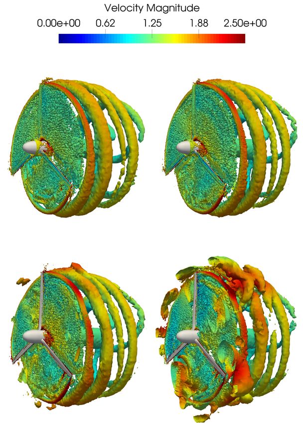
downstream turbine. Fig. 18 shows vorticity iso-surfaces based on Q-criterion. For clarity, vortex in front of the turbine
is clipped off for the turbulent inflow cases. As shown in Fig. 18, a large amount of tip vortex is generated due to the
rotation of the rotor. However, for the case of I = 15.
Thrust coefficient CT and power coefficient CP are the most important quantities for evaluating the tidal turbine
performance. CT and CP are given by
4F
CT = (13)
0.5ρw π D2 U02
4T ω
CP = (14)
0.5ρw π D2 U03
where F is thrust, T is torque, ρw is water density, D is the diameter of the turbine, U0 is the mean inflow water speed,
ω is the rotational speed.
540                        Q. Zhu and J. Yan / Computers and Mathematics with Applications 81 (2021) 532–546

                                          Fig. 14. Computational domain of the tidal turbine.

                                                  Fig. 15. Mesh of the tidal turbine.

   Fig. 19 shows the time history of the thrust and power coefficients for the uniform and turbulent inflow cases. For
the uniform case, the averaged experiment measurement from [66] is also plotted for comparison. The experiment data
we use to compare is the case of deep-tip immersion of 0.55D (D is diameter of the tidal turbine). The distance between
center of tidal turbine and water surface is big enough to neglect the free surface effect. Good agreement is achieved.
Please note that the experiments conducted in [66] only provides mean coefficients with uniform inflow conditions. From
Fig. 19, it is also seen that, the coefficient fluctuation increases as the inflow turbulence intensity increases. Table 6 shows
mean value and standard deviation of the thrust and power coefficients. The mean value of thrust and power coefficient
decreases as the increase of turbulence intensity. Experimental results from [69] also show the same trend for the mean
value of thrust and power coefficients (please note the experiment is performed using another similar three-blade turbine
design). It also shows that the influence of inflow turbulence on the mean thrust coefficient is smaller than that on the
mean power coefficient. Compared with mean values, the standard deviation is more sensitive to the inflow turbulence
intensity. For the thrust and power coefficients, standard deviations scale almost linearly with the turbulence intensity.
Experiment results in [69] show this trend as well.
Q. Zhu and J. Yan / Computers and Mathematics with Applications 81 (2021) 532–546              541

                                         Fig. 16. Instantaneous velocity magnitude of cut plane 1.

                               Table 6
                               Statistics of thrust and power coefficient of tidal turbine.
                                Inflow                   CT           CP            σCT          σCP
                                Uniform                  0.814        0.403         0.0112       0.0120
                                Experiment [66]          0.85         0.42          –            –
                                I=5%                     0.807        0.393         0.0238       0.0255
                                I=10%                    0.802        0.390         0.0396       0.0435
                                I=15%                    0.783        0.368         0.0594       0.0644

4. Conclusion

   A moving-domain CFD solver is developed by deploying ALE-VMS method with weak BC in FEniCS. The implementation
details are presented. Flow past a sphere with Re = 400 is simulated with moving meshes to validate the solver. Refinement
study shows that the results quickly converge to high-resolution DNS results. The solver is utilized to simulate tidal turbine
542 Q. Zhu and J. Yan / Computers and Mathematics with Applications 81 (2021) 532–546
Fig. 17. Instantaneous velocity magnitude of the middle plane (y = 0).Q. Zhu and J. Yan / Computers and Mathematics with Applications 81 (2021) 532–546 543
Fig. 18. Vorticity isosurface colored by velocity magnitude.
in both uniform inflow and turbulent inflow conditions. For the uniform inflow case, good agreement is achieved between
the experiment data and computational results. For the turbulent inflow cases, as the turbulence intensity increases, the
mean thrust coefficient decreases from 0.814 to 0.783 while the mean power coefficient decreases from 0.403 to 0.368. The
standard deviation of thrust coefficient increases from 0.0112 to 0.0594 while the standard deviation of power coefficient
increases from 0.0120 to 0.0644 from uniform inflow case to turbulent inflow case with I = 15%. The solver will be
open-sourced in the near future. Due to the flexibility and easiness of being upgraded, the solver can be widely applied
to offshore, and ocean engineering problems, where CFD calculations play an essential role.
Acknowledgments
The authors gratefully acknowledge the computing resources and startup funds provided by the University of Illinois
at Urbana–Champaign.544 Q. Zhu and J. Yan / Computers and Mathematics with Applications 81 (2021) 532–546
Fig. 19. Time history of thrust and power coefficients.Q. Zhu and J. Yan / Computers and Mathematics with Applications 81 (2021) 532–546 545
References
[1] M. Harrison, W. Batten, A. Bahaj, A blade element actuator disc approach applied to tidal stream turbines, in: OCEANS 2010 MTS/IEEE SEATTLE,
IEEE, 2010, pp. 1–8.
[2] L. Chen, J. Zang, A. Hillis, G. Morgan, A. Plummer, Numerical investigation of wave–structure interaction using OpenFOAM, Ocean Eng. 88 (2014)
91–109.
[3] Q. Xiong, S. Aramideh, A. Passalacqua, S.-C. Kong, Characterizing effects of the shape of screw conveyorsin gas–solid fluidized beds using
advanced numerical models, J. Heat Transfer 137 (6) (2015) 061008.
[4] Q. Xiong, S.-C. Kong, High-resolution particle-scale simulation of biomass pyrolysis, ACS Sustainable Chem. Eng. 4 (10) (2016) 5456–5461.
[5] Q. Xiong, Y. Yang, F. Xu, Y. Pan, J. Zhang, K. Hong, G. Lorenzini, S. Wang, Overview of computational fluid dynamics simulation of reactor-scale
biomass pyrolysis, ACS Sustainable Chem. Eng. 5 (4) (2017) 2783–2798.
[6] K. Hong, Y. Gao, A. Ullah, F. Xu, Q. Xiong, G. Lorenzini, Multi-scale CFD modeling of gas-solid bubbling fluidization accounting for sub-grid
information, Adv. Powder Technol. 29 (3) (2018) 488–498.
[7] Z. Wang, W. Yan, W.K. Liu, M. Liu, Powder-scale multi-physics modeling of multi-layer multi-track selective laser melting with sharp interface
capturing method, Comput. Mech. 63 (4) (2019) 649–661.
[8] A. Logg, K.-A. Mardal, G. Wells, Automated Solution of Differential Equations by the Finite Element Method: The FEniCS Book, vol. 84, Springer
Science & Business Media, 2012.
[9] S. Balay, K. Buschelman, V. Eijkhout, W.D. Gropp, D. Kaushik, M.G. Knepley, L.C. McInnes, B.F. Smith, H. Zhang, PETSC users manual, Technical
Report ANL-95/11-Revision 2.1. 5, Argonne National Laboratory, 2004.
[10] V. Hernandez, J.E. Roman, V. Vidal, SLEPC: A scalable and flexible toolkit for the solution of eigenvalue problems, ACM Trans. Math. Softw. 31
(3) (2005) 351–362.
[11] T.E. Tezduyar, Stabilization parameters and element length scales in SUPG and PSPG formulations, in: Book of Abstracts of an Euro Conference
on Numerical Methods and Computational Mechanics, Miskolc, Hungary, 2002.
[12] T.E. Tezduyar, Computation of moving boundaries and interfaces with interface-tracking and interface-capturing techniques, in: Pre-Conference
Proceedings of the Sixth Japan-US International Symposium on Flow Simulation and Modeling, Fukuoka, Japan, 2002.
[13] T.E. Tezduyar, Finite element methods for fluid dynamics with moving boundaries and interfaces, in: E. Stein, R.D. Borst, T.J.R. Hughes (Eds.),
Encyclopedia of Computational Mechanics, in: Volume 3: Fluids, John Wiley & Sons, 2004.
[14] T.E. Tezduyar, Finite elements in fluids: Stabilized formulations and moving boundaries and interfaces, Comput. & Fluids 36 (2007) 191–206,
http://dx.doi.org/10.1016/j.compfluid.2005.02.011.
[15] T.E. Tezduyar, T.J.R. Hughes, Finite element formulations for convection dominated flows with particular emphasis on the compressible Euler
equations, in: Proceedings of AIAA 21st Aerospace Sciences Meeting, AIAA Paper 83-0125, Reno, Nevada, 1983.
[16] Y. Bazilevs, V.M. Calo, T.J.R. Hughes, Y. Zhang, Isogeometric fluid–structure interaction: theory, algorithms, and computations, Comput. Mech.
43 (2008) 3–37.
[17] Y. Bazilevs, K. Takizawa, T.E. Tezduyar, Computational Fluid-Structure Interaction: Methods and Applications, Wiley, 2013.
[18] T.E. Tezduyar, K. Takizawa, Y. Bazilevs, Fluid–structure interaction and flows with moving boundaries and interfaces, in: Encyclopedia
Computational Mechanics, second ed., Wiley Online Library, 2018, pp. 1–53.
[19] K. Takizawa, T. Yabe, Y. Tsugawa, T.E. Tezduyar, H. Mizoe, Computation of free–surface flows and fluid–object interactions with the CIP method
based on adaptive meshless Soroban grids, Comput. Mech. 40 (2007) 167–183, http://dx.doi.org/10.1007/s00466-006-0093-2.
[20] Y. Bazilevs, V.M. Calo, J.A. Cottrell, T.J.R. Hughes, A. Reali, G. Scovazzi, Variational multiscale residual-based turbulence modeling for large eddy
simulation of incompressible flows, Comput. Methods Appl. Mech. Engrg. 197 (2007) 173–201.
[21] Y. Bazilevs, T.J.R. Hughes, NURBS-based isogeometric analysis for the computation of flows about rotating components, Comput. Mech. 43
(2008) 143–150.
[22] Y. Bazilevs, M.-C. Hsu, I. Akkerman, S. Wright, K. Takizawa, B. Henicke, T. Spielman, T.E. Tezduyar, 3d simulation of wind turbine rotors at full
scale. Part I: geometry modeling and aerodynamics, Internat. J. Numer. Methods Fluids 65 (2011) 207–235, http://dx.doi.org/10.1002/fld.2400.
[23] Y. Bazilevs, M.-C. Hsu, J. Kiendl, R. Wüchner, K.-U. Bletzinger, 3d simulation of wind turbine rotors at full scale. Part II: Fluid–structure interaction
modeling with composite blades, Internat. J. Numer. Methods Fluids 65 (2011) 236–253.
[24] Y. Bazilevs, M.-C. Hsu, K. Takizawa, T.E. Tezduyar, ALE-VMS And ST-VMS methods for computer modeling of wind-turbine rotor aerodynamics
and fluid–structure interaction, Math. Models Methods Appl. Sci. 22 (supp02) (2012) 1230002, http://dx.doi.org/10.1142/S0218202512300025.
[25] M.-C. Hsu, Y. Bazilevs, Fluid–structure interaction modeling of wind turbines: simulating the full machine, Comput. Mech. 50 (2012) 821–833.
[26] J. Yan, A. Korobenko, X. Deng, Y. Bazilevs, Computational free-surface fluid–structure interaction with application to floating offshore wind
turbines, Comput. & Fluids 141 (2016) 155–174.
[27] A. Korobenko, J. Yan, S. Gohari, S. Sarkar, Y. Bazilevs, FSI Simulation of two back-to-back wind turbines in atmospheric boundary layer flow,
Comput. & Fluids 158 (2017) 167–175.
[28] Y. Bazilevs, J. Yan, X. Deng, A. Korobenko, Computer modeling of wind turbines: 2. Free-surface FSI and fatigue-damage, Arch. Comput. Methods
Eng. (2018) 1–15.
[29] M.-C. Hsu, I. Akkerman, Y. Bazilevs, Wind turbine aerodynamics using ALE-VMS: Validation and role of weakly enforced boundary conditions,
Comput. Mech. 50 (2012) 499–511.
[30] T.M. van Opstal, J. Yan, C. Coley, J.A. Evans, T. Kvamsdal, Y. Bazilevs, Isogeometric divergence-conforming variational multiscale formulation of
incompressible turbulent flows, Comput. Methods Appl. Mech. Engrg. 316 (2017) 859–879.
[31] Y. Bazilevs, I. Akkerman, Large eddy simulation of turbulent Taylor–Couette flow using isogeometric analysis and the residual-based variational
multiscale method, J. Comput. Phys. 229 (9) (2010) 3402–3414.
[32] J. Yan, S. Lin, Y. Bazilevs, G.J. Wagner, Isogeometric analysis of multi-phase flows with surface tension and with application to dynamics of
rising bubbles, Comput. & Fluids (2018).
[33] J. Yan, W. Yan, S. Lin, G.J. Wagner, A fully coupled finite element formulation for liquid–solid–gas thermo-fluid flow with melting and
solidification, Comput. Methods Appl. Mech. Engrg. 336 (2018) 444–470.
[34] Y. Bazilevs, A. Korobenko, J. Yan, A. Pal, S.M.I. Gohari, S. Sarkar, ALE–VMS Formulation for stratified turbulent incompressible flows with
applications, Math. Models Methods Appl. Sci. 25 (2015) 1540011.
[35] J. Yan, A. Korobenko, A. Tejada-Martínez, R. Golshan, Y. Bazilevs, A new variational multiscale formulation for stratified incompressible turbulent
flows, Comput. & Fluids 158 (2017) 150–156.
[36] S. Xu, N. Liu, J. Yan, Residual-based variational multi-scale modeling for particle-laden gravity currents over flat and triangular wavy terrains,
Comput. & Fluids (2019).
[37] F. Xu, D. Schillinger, D. Kamensky, V. Varduhn, C. Wang, M.-C. Hsu, The tetrahedral finite cell method for fluids: Immersogeometric analysis
of turbulent flow around complex geometries, Comput. & Fluids (2015).546 Q. Zhu and J. Yan / Computers and Mathematics with Applications 81 (2021) 532–546
[38] M.-C. Hsu, D. Kamensky, Y. Bazilevs, M.S. Sacks, T.J.R. Hughes, Fluid–structure interaction analysis of bioprosthetic heart valves: significance of
arterial wall deformation, Comput. Mech. 54 (2014) 1055–1071, http://dx.doi.org/10.1007/s00466-014-1059-4.
[39] K. Takizawa, T.E. Tezduyar, A. Buscher, S. Asada, Space–time fluid mechanics computation of heart valve models, Comput. Mech. 54 (2014)
973–986, http://dx.doi.org/10.1007/s00466-014-1046-9.
[40] D. Kamensky, M.-C. Hsu, D. Schillinger, J.A. Evans, A. Aggarwal, Y. Bazilevs, M.S. Sacks, T.J. Hughes, An immersogeometric variational framework
for fluid–structure interaction: Application to bioprosthetic heart valves, Comput. Methods Appl. Mech. Engrg. 284 (2015) 1005–1053.
[41] K. Takizawa, T.E. Tezduyar, H. Uchikawa, T. Terahara, T. Sasaki, K. Shiozaki, A. Yoshida, K. Komiya, G. Inoue, Aorta flow analysis and heart valve
flow and structure analysis, in: Frontiers in Computational Fluid-Structure Interaction and Flow Simulation, Springer, 2018, pp. 29–89.
[42] F. Xu, S. Morganti, R. Zakerzadeh, D. Kamensky, F. Auricchio, A. Reali, T.J. Hughes, M.S. Sacks, M.-C. Hsu, A framework for designing patient-
specific bioprosthetic heart valves using immersogeometric fluid–structure interaction analysis, Int. J. Numer. Methods Biomed. Eng. 34 (4)
(2018) e2938.
[43] K. Takizawa, T.E. Tezduyar, T. Kuraishi, Multiscale Space–Time methods for thermo-fluid analysis of a ground vehicle and its tires, Math. Models
Methods Appl. Sci. 25 (12) (2015) 2227–2255.
[44] T. Kuraishi, K. Takizawa, T.E. Tezduyar, Tire aerodynamics with actual tire geometry, road contact and tire deformation, Comput. Mech. 63 (6)
(2019) 1165–1185.
[45] F. Xu, G. Moutsanidis, D. Kamensky, M.-C. Hsu, M. Murugan, A. Ghoshal, Y. Bazilevs, Compressible flows on moving domains: Stabilized
methods, weakly enforced essential boundary conditions, sliding interfaces, and application to gas-turbine modeling, Comput. & Fluids 158
(2017) 201–220.
[46] F. Xu, Y. Bazilevs, M.-C. Hsu, Immersogeometric analysis of compressible flows with application to aerodynamic simulation of rotorcraft, Math.
Models Methods Appl. Sci. 29 (05) (2019) 905–938.
[47] J. Yan, B. Augier, A. Korobenko, J. Czarnowski, G. Ketterman, Y. Bazilevs, FSI modeling of a propulsion system based on compliant hydrofoils
in a tandem configuration, Comput. & Fluids (2015) Published online. http://dx.doi.org/10.1016/j.compfluid.2015.07.013.
[48] B. Augier, J. Yan, A. Korobenko, J. Czarnowski, G. Ketterman, Y. Bazilevs, Experimental and numerical FSI study of compliant hydrofoils, Comput.
Mech. 55 (2015) 1079–1090, http://dx.doi.org/10.1007/s00466-014-1090-5.
[49] T.A. Helgedagsrud, Y. Bazilevs, K.M. Mathisen, J. Yan, O.A. Øseth, Modeling and simulation of bridge-section buffeting response in turbulent
flow, Math. Models Methods Appl. Sci. (2019).
[50] V. Kalro, T.E. Tezduyar, A parallel 3D computational method for fluid–structure interactions in parachute systems, Comput. Methods Appl. Mech.
Engrg. 190 (2000) 321–332, http://dx.doi.org/10.1016/S0045-7825(00)00204-8.
[51] T. Kanai, K. Takizawa, T.E. Tezduyar, T. Tanaka, A. Hartmann, Compressible-flow geometric-porosity modeling and spacecraft parachute
computation with isogeometric discretization, Comput. Mech. 63 (2) (2019) 301–321.
[52] K. Takizawa, T.E. Tezduyar, T. Kanai, Porosity models and computational methods for compressible-flow aerodynamics of parachutes with
geometric porosity, Math. Models Methods Appl. Sci. 27 (04) (2017) 771–806.
[53] T.J. Hughes, Recent progress in the development and understanding of SUPG methods with special reference to the compressible euler and
Navier-Stokes equations, Int. J. Numer. Methods fluids 7 (11) (1987) 1261–1275.
[54] T.E. Tezduyar, Stabilized finite element formulations for incompressible flow computations, in: Advances in Applied Mechanics, vol. 28, Elsevier,
1991, pp. 1–44.
[55] M. Olshanskii, G. Lube, T. Heister, J. Löwe, Grad–div stabilization and subgrid pressure models for the incompressible Navier–Stokes equations,
Comput. Methods Appl. Mech. Engrg. 198 (49–52) (2009) 3975–3988.
[56] T.E. Tezduyar, Y. Osawa, Finite element stabilization parameters computed from element matrices and vectors, Comput. Methods Appl. Mech.
Engrg. 190 (3–4) (2000) 411–430.
[57] O. Colomés, S. Badia, R. Codina, J. Principe, Assessment of variational multiscale models for the large eddy simulation of turbulent incompressible
flows, Comput. Methods Appl. Mech. Engrg. 285 (2015) 32–63.
[58] M.S. Alnæs, UFL: a finite element form language, in: Automated Solution of Differential Equations By the Finite Element Method, Springer,
2012, pp. 303–338.
[59] R.C. Kirby, FIAT: numerical construction of finite element basis functions, in: Automated Solution of Differential Equations By the Finite Element
Method, Springer, 2012, pp. 247–255.
[60] M.S. Alnæs, A. Logg, K.-A. Mardal, UFC: a finite element code generation interface, in: Automated Solution of Differential Equations By the
Finite Element Method, Springer, 2012, pp. 283–302.
[61] I.M. Wilbers, K.-A. Mardal, M.S. Alnæs, Instant: just-in-time compilation of C/C++ in Python, in: Automated Solution of Differential Equations
By the Finite Element Method, Springer, 2012, pp. 257–272.
[62] A. Logg, G.N. Wells, J. Hake, DOLFIN: A C++/Python finite element library, in: Automated Solution of Differential Equations By the Finite Element
Method, Springer, 2012, pp. 173–225.
[63] K.E. Jansen, S.S. Collis, C. Whiting, F. Shaki, A better consistency for low-order stabilized finite element methods, Comput. Methods Appl. Mech.
Engrg. 174 (1–2) (1999) 153–170.
[64] S. Lee, A numerical study of the unsteady wake behind a sphere in a uniform flow at moderate Reynolds numbers, Comput. & Fluids 29 (6)
(2000) 639–667.
[65] V. Gushchin, A. Kostomarov, P. Matyushin, E. Pavlyukova, Direct numerical simulation of the transitional separated fluid flows around a sphere
and a circular cylinder, J. Wind Eng. Ind. Aerodyn. 90 (4–5) (2002) 341–358.
[66] A. Bahaj, W. Batten, G. McCann, Experimental verifications of numerical predictions for the hydrodynamic performance of horizontal axis marine
current turbines, Renew. Energy 32 (15) (2007) 2479–2490.
[67] J. Yan, X. Deng, A. Korobenko, Y. Bazilevs, Free-surface flow modeling and simulation of horizontal-axis tidal-stream turbines, Comput. & Fluids
158 (2017) 157–166.
[68] N. Jarrin, R. Prosser, J.-C. Uribe, S. Benhamadouche, D. Laurence, Reconstruction of turbulent fluctuations for hybrid RANS/LES simulations using
a synthetic-eddy method, Int. J. Heat Fluid Flow 30 (3) (2009) 435–442.
[69] P. Mycek, B. Gaurier, G. Germain, G. Pinon, E. Rivoalen, Experimental study of the turbulence intensity effects on marine current turbines
behaviour. Part I: One single turbine, Renew. Energy 66 (2014) 729–746.You can also read