Two-layer Thermally Driven Turbulence: Mechanisms for Interface Breakup
←
→
Page content transcription
If your browser does not render page correctly, please read the page content below
This draft was prepared using the LaTeX style file belonging to the Journal of Fluid Mechanics   1
arXiv:2005.05633v2 [physics.flu-dyn] 17 Nov 2020

                                                          Two-layer Thermally Driven Turbulence:
                                                            Mechanisms for Interface Breakup
                                                      Hao-Ran Liu1 , Kai Leong Chong1 , Qi Wang1,2 , Chong Shen Ng1 ,
                                                               Roberto Verzicco3,4,1 and Detlef Lohse1,5, †
                                                      1
                                                        Physics of Fluids Group and Max Planck Center Twente for Complex Fluid Dynamics,
                                                        MESA+Institute and J. M. Burgers Centre for Fluid Dynamics, University of Twente,
                                                                          P.O. Box 217, 7500AE Enschede, The Netherlands
                                                      2
                                                        Department of Modern Mechanics, University of Science and Technology of China, Hefei
                                                                                             230027, China
                                                         3
                                                           Dipartimento di Ingegneria Industriale, University of Rome “Tor Vergata”, Via del
                                                                                   Politecnico 1, Roma 00133, Italy
                                                                4
                                                                  Gran Sasso Science Institute - Viale F. Crispi, 7 67100 L’Aquila, Italy
                                                   5
                                                     Max Planck Institute for Dynamics and Self-Organization, Am Fassberg 17, 37077 Göttingen,
                                                                                                Germany

                                                                                 (Received xx; revised xx; accepted xx)

                                                   It is commonly accepted that the breakup criteria of drops or bubbles in turbulence is
                                                   governed by surface tension and inertia. However, also buoyancy can play an important
                                                   role at breakup. In order to better understand this role, here we numerically study
                                                   two-dimensional Rayleigh-Bénard convection for two immiscible fluid layers, in order to
                                                   identify the effects of buoyancy on interface breakup. We explore the parameter space
                                                   spanned by the Weber number 5 6 W e 6 5000 (the ratio of inertia to surface tension)
                                                   and the density ratio between the two fluids 0.001 6 Λ 6 1, at fixed Rayleigh number
                                                   Ra = 108 and Prandtl number P r = 1. At low W e, the interface undulates due to plumes.
                                                   When W e is larger than a critical value, the interface eventually breaks up. Depending on
                                                   Λ, two breakup types are observed: The first type occurs at small Λ ≪ 1 (e.g. air-water
                                                   systems) when local filament thicknesses exceed the Hinze length scale. The second,
                                                   strikingly different, type occurs at large Λ with roughly 0.5 < Λ 6 1 (e.g. oil-water
                                                   systems): The layers undergo a periodic overturning caused by buoyancy overwhelming
                                                   surface tension. For both types the breakup, criteria can be derived from force balance
                                                   arguments and show good agreement with the numerical results.

                                                   Key words:

                                                   1. Introduction
                                                      Liquid can break up or fragment in multiphase turbulence (Deane & Stokes 2002;
                                                   Villermaux 2007; Wang et al. 2019; Villermaux 2020). This physical phenomenon is
                                                   very important for raindrops (Villermaux & Bossa 2009; Josserand & Zaleski 2003),
                                                   for ocean waves and the resulting spray (Veron 2015), and even for the transmis-
                                                   sion of virus-laden droplets during coughing or sneezing (Bourouiba 2020; Chong et al.
                                                   2020). Once the physical mechanisms governing this important phenomenon are un-
                                                                       † Email address for correspondence: d.lohse@utwente.nl
2 H.-R. Liu, K. L. Chong, Q. Wang, C. S. Chong, R. Verzicco and D. Lohse derstood, one can deduce quantitative criteria for the breakup to occur. In turbu- lence, for drops or bubbles the breakup criteria can be deduced from the balance of inertial and surface tension forces, as developed in the Kolmogorov-Hinze theory (Kolmogorov 1949; Hinze 1955). This theory well predicts the breakup criteria in experi- mental and numerical results in various flow systems, e.g., homogeneous isotropic turbu- lence (Martı́nez-Bazán et al. 1999; Perlekar et al. 2012; MuKolmogorov-Hinzeerjee et al. 2019), shear flows (Rosti et al. 2019), pipe flows (Hesketh et al. 1991) and ocean waves (Deane & Stokes 2002; Deike et al. 2016). Whilst the classical Kolmogorov-Hinze theory considers only surface tension and inertial forces, in many multiphase turbulent flows also buoyancy can play an important role. Examples of multiphase buoyant turbulence include the hotspots and superswells in Earth’s mantle (Davaille 1999; Tackley 2000) and even flows during sneezing and exhalation (Bourouiba et al. 2014). In such flows, the breakup of the interface between the fluids is the key phenomenon. Yet, the exact mechanisms that drives interface breakup when buoyancy is crucial is unknown. The objective of the present work is to shed light on this mechanism. As examples for turbulent flow where buoyancy is important and at the same time can easily be tuned, we take thermal convection, namely Rayleigh-Bénard (RB) convection (Ahlers et al. 2009; Lohse & Xia 2010; Chillà & Schumacher 2012) of two immiscible fluids. We numerically investigate the breakup mechanisms of the interface between the two immiscible fluids. The immiscible fluids are first arranged in two layers according to their densities and then heated from below and cooled from above. Most previous studies of such two- layer RB convection were conducted in the non-turbulent regime (Nataf et al. 1988; Prakash & Koster 1994; Busse & Petry 2009; Diwakar et al. 2014). Experimental studies in the turbulent regime were reported by Xie & Xia (2013), who focused on the flow struc- tures in each layer and the coupling modes between the flows in the two layers, including viscous coupling and thermal coupling. Besides the classical rectangular/cylindrical con- figuration, the two-layer RB convection in spherical-shell geometry was also numerically studied by Yoshida & Hamano (2016). However, these previous studies only considered the case for strong surface tension, where the interface between the layers does not break up. In this study we will for the first time explore the case with interface breakup, which happens when surface tension is sufficiently small. The control parameters of two-layer RB convection are the density ratio Λ between two fluids and the Weber number W e, which is the ratio of inertia to surface tension. We will keep the Prandtl number P r (a material property) and the Rayleigh number Ra (the dimensionless temperature difference between the plates) fixed, at values allowing for considerable turbulence. Our main result will be the phase diagram in the parameter space (W e, Λ), in which we identify the non-breakup and breakup regimes. At increasing W e, we observe two distinct types of interface breakup. At small Λ ≪ 1, the mechanism is well-described by the Kolmogorov-Hinze theory. However, at large 0.5 < Λ 6 1, the breakup is dominated by a balance between buoyancy and surface tension forces, leading to a periodic overturning-type breakup. The organization of this paper is as follows. The numerical methodology is introduced in Section 2. Then in Section 3, we validate our code by studying droplet fragmentation in thermal turbulence and favourably compare the results to the Kolmogorov-Hinze theory. The main results on the interface breakup in two-layer RB turbulence are presented in Section 4, including a discussion of the first and second types of interface breakup in Section 4.1 and Section 4.2, respectively, and the analysis of the critical Weber number for interface breakup in Section 4.3. We finalise and further discuss our findings in Section 5.
Two-layer Thermally Driven Turbulence: Mechanisms for Interface Breakup             3
2. Methodology: Cahn-Hilliard approach coupled to finite difference
   scheme
   In this study, we performed the simulations in a two-dimensional (2D) rectangular
domain with aspect ratio Γ = 2 (width divided by height). Although 2D RB convection is
different from 3D one, it still captures many essential features thereof (van der Poel et al.
2013). The direct numerical simulations solver for the Navier-Stokes equations is a second-
order finite-difference open source solver (Verzicco & Orlandi 1996; van der Poel et al.
2015), namely AFiD, which has been well validated and used to study various turbulent
flows (Stevens et al. 2018; Zhu et al. 2018b; Blass et al. 2020; Wang et al. 2020a,b). To
simulate multiphase turbulent flows, we combine AFiD with the phase-field method
(Jacqmin 1999; Ding et al. 2007; Liu & Ding 2015), which has also been successfully
applied to the interfacial (Liu et al. 2018; Zhu et al. 2017; Chen et al. 2018, 2020) and
turbulent flows (Soligo et al. 2019a; Roccon et al. 2019).
   We consider two immiscible fluid layers of the same volume placed in the domain,
named fluid H for the heavier fluid initially at the bottom and fluid L for the lighter fluid
initially at the top. The mathematically sharp interface between two fluids is modeled
by a diffuse interface with finite thickness, and can be represented by contours of the
volume fraction C of fluid H. The corresponding volume fraction of fluid L is 1 − C. The
evolution of C is governed by the Cahn-Hilliard equations,
                                    ∂C              1 2
                                       + ∇ · (uC) =    ∇ ψ,                             (2.1)
                                    ∂t              Pe
where u is the flow velocity, and ψ = C 3 − 1.5C 2 + 0.5C − Cn2 ∇2 C is the chemical
potential. The Cahn number Cn = 0.75h/D, where h is the mesh size and D the domain
height, and the Péclet number P e = 0.9/Cn are set the same as in Liu et al. (2017);
Li et al. (2020). To overcome the mass loss in the phase-field method, a correction method
as proposed by Wang et al. (2015) is used. This correction method resembles that used
in Soligo et al. (2019b) and exhibits good performance (see Section 3).
  The motion of the fluids is governed by the Navier-Stokes equation, heat transfer
equation and continuity,

                                     r
           ∂u                              Pr                                 ρ
   ρ          + u · ∇u       = −∇P +          ∇ · [µ(∇u + ∇uT )] + Fst + ρ θ −     j,   (2.2)
           ∂t                              Ra                                  Fr
                                               r
                               ∂θ                     1   1
                                  + u · ∇θ =                 ∇ · (k∇θ),                 (2.3)
                               ∂t                  P rRa ρCp

                                               ∇ · u = 0,                               (2.4)
here given in non-dimensionalized form. We have used the material properties of fluid
H, the domain height√ D, the temperature difference ∆ between plates, and the free-
fall velocity U = αgD∆ to make these equations dimensionless, where α is the
thermal expansion coefficient of fluid H and g the gravitational acceleration. Then we
define ρ = C + Λ(1 − C) as the dimensionless density, P the dimensionless pressure, µ
the dimensionless dynamic viscosity, Cp the√dimensionless specific heat capacity, k the
dimensionless thermal conductivity, Fst = 6 2ψ∇C/(Cn We) the dimensionless surface
tension force, θ the dimensionless temperature, j the unit vector in vertical direction.
The superscript T stands for the transpose. Note that ρ, µ, Cp and k in general vary in
space.
   In thermal flows, the density also depends on the temperature, so the dimensional
4 H.-R. Liu, K. L. Chong, Q. Wang, C. S. Chong, R. Verzicco and D. Lohse Figure 1. Snapshot with the advecting drops in Rayleigh-Bénard convection at density ratio Λ = 1 and the system Weber number W e = 16000. Drops are in gray, and the red and blue lines denote the plates with non-dimensional temperature θ = 1 and 0, respectively. The corresponding movie is shown as Supplementary Material. density is defined as ρ̂ = ρ̂H (T )C + ρ̂L (T )(1−C), where the subscripts H and L represent fluid H and fluid L, respectively, and ρ̂i (T ) = [1 − α(T − Tc )]ρ̂i (Tc ) with Tc being the temperature on the top cold plate. Then we rewrite the dimensional density as ρ̂ = [ρ− α(T − Tc )ρ]ρ̂H (Tc ). Further considering the Oberbeck-Boussinesq approximation in the Navier-Stokes equation (2.2), we have the dimensionless density ρ in the inertia term, ρθ, as the buoyancy term, and ρ/F r as the gravity term, which cannot be ignored as in the single phase simulation, due to the different densities of the fluids. Furthermore, we only consider the case without phase transition. The properties of fluid H and fluid L are set as follows: Their density ratio is Λ = ρL /ρH 6 1. Except for the density ρ, all other properties of the two fluids are the same. The other dimensionless parameters are W e = ρH U 2 D/σ, Ra = αgD3 ∆/(νκ), P r = ν/κ, the Froude number F r = U 2 /(gD) (the ratio of inertia to gravity). Here σ is the surface tension coefficient, ν = µ/ρ the kinematic viscosity, and κ = k/(ρCp ) the thermal diffusivity. We fix Ra = 108 , P r = 1, F r = 1 and Γ = 2 (these values chosen to both ensure flows in the turbulent regime and simplify the simulations), and only vary W e from 5 to 5000 and Λ from 0.001 (e.g. air-water system) to 1 (e.g. oil-water system). The boundary conditions at the top and bottom plates are set as ∂C/∂j = 0, j·∇ψ = 0, no-slip velocities and fixed temperature θ = 0 (top) and 1 (bottom). Periodic conditions are used in the horizontal direction. All the simulations begin with the same initial velocity and temperature fields, which originates from a well developed turbulent flow at W e = 5 and Λ = 1. Uniform grids with 1000 × 500 gridpoints are used, which are sufficient for Ra = 108 and P r = 1, consistent with the grid resolution checks in Zhang et al. (2017). The details of the discretizations can be found in Ding et al. (2007); Verzicco & Orlandi (1996); M. S. Dodd (2014). 3. Droplet fragmentation in turbulent flow We have verified our code against the existing theory from the literature. In this section RB convection with drops are simulated. Initially, the temperature field has a linear profile, the velocity field is set to 0, and a big drop of fluid H with a diameter of 0.5D is placed at the center of the domain. The plates are superhydrophobic for fluid H, i.e. C = 0 is used on both plates in the verification cases. We set Λ = 1 and W e from 2000 to 16000, and use uniform grids with 2000 × 1000 gridpoints. Note that the value of W e is large because it is a system Weber number, and the local Weber number of drops calculated from simulations is of the order of 1.
Two-layer Thermally Driven Turbulence: Mechanisms for Interface Breakup 5
-4 -1
(a) 10 (b) 10 (c)
X X XX
X
0.4
XXXX
XXX -10/3 -3/5
10-2
XXXXX
XXXX
(S/D) We
10-5
XX
XX
X
XXX
XX
X X
Smax /D
X XX
XXX
PDF
XXX
XXXX
XXXX
X
Emass
XXXX
XX
XXXX XXX
XXXX
X
XXXXXX
XX X
10-3
XXXX
X
X X XXXX
XXXX
X XXX
10-6 X X
XX
XXXX XX
X X XX X
X XXX X
XX
X
XX XXX
X
X XX 0.1
10-4
XXXX
-7 X
XXX X
10
0 100 200 0.01 0.1 103 104
t S/D We
Figure 2. (a) Temporal evolution of Mass error Emass and (b) probability density function
p
(PDF) of the drop size S/D at W e = 16000, where D is the domain height and S = 2 A/π
with A being the drop area. (c) Maximal drop size Smax /D as function of W e, where Smax
is measured in the same way as in Hinze (1955), that is the diameter of the equivalent drop
occupying 95% of the total dispersed area.
From the snapshot with the advecting drops in figure 1, we observe the large scale
circulation, which is well known from single phase convection (Krishnamurti & Howard
1981; Xi et al. 2004; Zhu et al. 2018a; Xie et al. 2018). Figure 2(b) displays the distri-
bution of the drop size S, which follows the scaling law (S/D)−10/3 (Garrett et al. 2000;
Yu et al. 2020) valid for large drops. This scaling is consistent with experimental and
other numerical results where the breakup of waves (Deane & Stokes 2002; Deike et al.
2016) or of a big drop (MuKolmogorov-Hinzeerjee et al. 2019) was studied. Moreover,
the maximal size of drops Smax (see figure 2c) well agrees with the Kolmogorov-Hinze
scaling law Smax /D ∼ W e−3/5 , which originates from Hinze (1955),
53
σ 2
SHinze ∼ ǫ− 5 , (3.1)
ρ
where SHinze is the Hinze length scale and ǫ the energy dissipation rate of the turbulent
flow. In the Kolmogorov-Hinze theory, one assumption is that the local Weber number
defined by the size and velocity of the drops adjusts such that it is W elocal ∼ O(1).
Indeed, in our simulations the local drop size adjusts correspondingly, so this assumption
is fulfilled. The second assumption is that the flow exhibits inertial subrange scaling
in the region of wave lengths comparable to the size of the largest drops. The spatial
location where this assumption holds in RB convection is in the bulk region of convection
(Lohse & Xia 2010). Therefore, the Kolmogorov-Hinze theory can indeed also be reason-
ably applied to 2D RB convection. At the same time the results show that the code and
the approach give consistent results. Besides, figure 2(a) shows the temporal evolution of
mass error Emass = |Mt − M0 |/M0 , where Mt is the mass of fluid H at time t and and
M0 the initial mass. The results indicate good mass conservation.
4. Interfacial breakup in two-layer turbulent thermal convection
In two-layer RB convection with an initially smooth interface between the two fluids
(Xie & Xia 2013), the densities of the fluids depend on both Λ and the local temperature.
At small Λ, for example, the air-water system with Λ = 0.001, fluid H (water) is always
heavier than fluid L (air) even if fluid H, as the bottom layer, is hotter. In contrast, at
large Λ, e.g., an oil-water system with Λ ≈ 1, fluid H (water) is hotter than fluid L (oil),
so it can be lighter. So depending on the value of Λ two distinct types of flow phenomena
emerge.6 H.-R. Liu, K. L. Chong, Q. Wang, C. S. Chong, R. Verzicco and D. Lohse
0 0.5 1
(a) θ
1 1
We=5
Fluid L
0.5
0.5 0.5
y
Fluid H
0 0
(b) 1 1
We=600
0.5
0.5 0.5
y
0 0
(c) 1 1
We=2000
0.5
0.5 0.5
y
0 0
0 1 2 0 0.25 0.5 0.75 1
x θ
Figure 3. First type of interface breakup occurring for small Λ ≪ 1: Temperature field and
average temperature profile of two-layer Rayleigh-Bénard convection at Λ = 0.3 for (a) W e = 5,
(b) W e = 600 and (c) W e = 2000. The corresponding movies are shown as Supplementary
Material.
(a) 0.70 (b) 2
∗
Sfila SHinze ∗
N aver
0.25 1
∗∗
0.70
0
∗
0.25 0 1000 2000 3000
0.70 1.42 We
Figure 4. (a) Detachment process of a drop at W e = 2000. (b) Time-averaged number of
the drops of fluid L emerged in fluid H for various W e, where the empty circles denote the
non-breakup regime and stars the breakup regime.
4.1. First type of interface breakup occurring for small Λ ≪ 1
At small Λ, fluid H forms the bottom layer and fluid L the top one and large scale
circulations are observed in each layer between the interface and the respective plate, as
seen in figure 3(a). With increasing W e, i.e. decreasing effects of surface tension compared
to inertia, the interface becomes more unstable. At low W e (figure 3a), the interface only
slightly deforms because the surface tension is large enough to resist the inertia, such
that the convection rolls are well-ordered. The temperature profile is similar to thatTwo-layer Thermally Driven Turbulence: Mechanisms for Interface Breakup 7
(a) 1 (b) 1
We=20 We=30 t1
Fluid L
Fluid H
0 0
0 1 2 0 1 2
(c) 1
Fluid H t2 t3 t4 t5
Fluid L
0
0 2 0 2 0 2 0 2
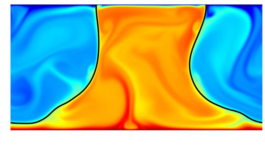
Figure 5. Second type of interface breakup occurring for large 0.5 < Λ 6 1: Snapshots at
Λ = 0.8 for two different W e. (a) Wavy interface for W e = 20. (b) Breakup and (c) overturning
of interface for W e = 30 at different times t1 = 617, t2 = 640, t3 = 661, t4 = 730 and t5 = 803.
ti are also marked in figure 6. The color map is the same as in figure 3. The corresponding
movies are shown as Supplementary Material.
obtained from two-layer RB convection experiments (Davaille 1999). As W e increases
(figure 3b), the interface undulates due to the plumes. Each crest and trough on the
interface is caused by a rising, or respectively settling plume in the heavier fluid H.
In this situation, inertia is resisted by gravity together with surface tension. When W e
keeps increasing (figure 3c), the interface eventually breaks up and drops detach from
the interface between two layers.
This “first type of interface breakup” (as we call it) occurs at small Λ. The process
of the breakup begins from a settling plume in fluid H thanks to which the interface
is pulled downwards, leading to a filament (or trough) on the interface (see figure 4a).
If the filament length Sf ila (defined in figure 4a) grows larger than the Hinze length
scale SHinze , the filament will pinch off from the interface. Within the Kolmogrov-Hinze
theory (Hinze 1955), the Hinze length scale SHinze in (3.1) is determined by the energy
dissipation rate ǫ of the turbulent flow. As seen from figure 3(c), more drops of fluid L
exist in fluid H than of fluid H in fluid L. This finding resembles the breakup of the
ocean waves (Deane & Stokes 2002), leading to more bubbles in water than drops in air.
The reason is that SHinze is smaller in fluid H than in fluid L as ρH > ρL .
4.2. Second type of interface breakup occurring for large 0.5 < Λ 6 1
We now come to the large Λ ≈ 1 case: Since fluid H carries hotter fluid than fluid
L, due to thermal expansion it can become lighter than fluid L, inverting the original
density contrast at equal temperature. In this situation, buoyancy drives fluid H upwards
and fluid L downwards. This leads to wave crests and troughs, as shown in figure 5. If
W e is low (figure 5a), the surface tension can maintain a stable interface, though it is
wobbling. However, if W e increases (figure 5b), the wobbling wave on the interface can
amplify more and more until it finally touches the upper and/or lower plate and breaks
up. We call this type of interface breakup the “second type of breakup”.
For this second type of interface breakup, the breakup process is strikingly different
from the first type. A periodic overturning is observed both in the fluid dynamics and
in the heat transfer (see figure 5c and figure 6): After interface breakup at t1 , fluid H
initially at the bottom gradually rises above fluid L and finally contacts the upper cold
plate. The increased wetted area of the hotter fluid on the upper cold plate causes a8 H.-R. Liu, K. L. Chong, Q. Wang, C. S. Chong, R. Verzicco and D. Lohse
80 50 2
W/D
Nu
60 10 0
600 700
Nu
40 t2
t1 t4 t5
20
0
t3
200 400 600 800 1000
t
Figure 6. Temporal evolution of the Nusselt number N u at the bottom plate for W e = 20
(black) and W e = 30 (blue). The inset shows a zoom of the temporal evolution of N u for
W e = 30 and the corresponding wetted length function W/D of fluid H at the top plate.
strong enhancement of the Nusselt number N u, in the shown case 5 times of N u without
breakup, as shown in figure 6. Then, fluid H on the top gets cooler and thus heavier,
while fluid L at the bottom warmer and thus lighter. Once again, the breakup occurs
after t3 and the fluids swap their positions (see figure 5c). Since fluid L is lighter than
fluid H at the same temperature, it is easier to rise and touch the cold plate. Thus, with
fluid L as the bottom layer, the temperature of the bottom layer during the breakup
is lower than that when fluid H is the bottom layer. This is also reflected in the heat
transfer. The peak of N u after t3 is smaller, only 3 times of N u without breakup, and
the preparation time for breakup from t2 to t3 is shorter than that from t4 to t5 .
4.3. Critical Weber number for interface breakup
The full phase diagram in the parameter space (W e, Λ) – revealing when and what
regime occurs – is plotted in figure 7. When W e is larger than a certain critical value W ec ,
which depends on Λ, the interface breaks up. It is noteworthy that the transition between
the non-breakup and breakup regimes show two distinct trends, which correspond to the
two above identified types of interface breakup, respectively. The natural question that
arises here is then: What sets the critical value W ec at given Λ?
In the first type of interface breakup (small Λ ≪ 1), detaching drops are generated
from the initial interface when the filament length Sf ila is of the order of the Hinze length
scale SHinze . Sf ila is estimated by analyzing the force balance: the sum of gravity and
surface tension force counteracts the inertial force,
σ 2
δρ gSf ila + ∼ ρH U H , (4.1)
Sf ila
p
where UH = αg(D/2)(∆/2) and δρ is the density difference from the bottom (fluid
H) to the top (fluid L) of the filament. We define δρ = ρH (TH ) − ρL (TL ), where Ti is
the temperature of fluid i. We further found that the value of gravity is one order of
magnitude greater than surface tension based on the data of cases near the transition
region in the first type. This indicates that the generation of the filament is dominated by
gravity and inertia. Therefore we neglect the term σ/Sf ila in (4.1). Note however that theTwo-layer Thermally Driven Turbulence: Mechanisms for Interface Breakup 9
1 ∗∗ ∗ ∗ ∗
∗ ∗ ∗ ∗
0.8 ∗ ∗∗ ∗ ∗
∗ ∗ ∗
0.6 ∗ ∗∗ ∗
Λ ∗ ∗
0.4 ∗∗ ∗
∗
∗∗∗∗∗
0.2 ∗∗∗∗∗ ∗
∗∗∗∗∗
0 0 ∗∗∗
∗ ∗∗∗∗
10 101 102 103 104
We
Figure 7. Phase diagram in the W e−Λ parameter space. Empty circles denote the non-breakup
regime and stars the interface breakup regime. Symbols with boldface are the cases shown in
figure 3 and 5. The gray shadow is a guide to the eye. The red and green lines denote the criteria,
(4.3) with prefactor 1590 and (4.6) with prefactor 13.3, for the first and second type of interface
breakup, respectively. The solid parts of the lines, where the theory is supposed to hold, indeed
nicely agree with the numerical results.
surface tension force still plays an important role to determine SHinze in (3.1). Combining
(4.1), (3.1) and the exact relation ǫ = ν 3 /D4 (N u − 1)RaP r−2 (Shraiman & Siggia 1990;
Ahlers et al. 2009), the dimensionless form of Sf ila ∼ SHinze yields
−1 − 25
1 1 − 53 Nu − 1
− θH −Λ − θL ∼ W ec √ , (4.2)
Fr Fr RaP r
with the non-dimensional temperatures θi = (Ti − Tc )/∆ with i being H and L. θH and
θL are both taken as 0.5 given that the filament is generated near the interface, where
the temperature is 0.5. To further simplify (4.2), N u is regarded as constant because the
simulation data show that N u varies only within 15% in the non-breakup regime. Given
that the N u, Ra, P r and F r are all constant, the criteria for the first type of interface
breakup simplifies to
5
W ec ∼ (1 − Λ) 3 . (4.3)
In the second type of interface breakup (large Λ ≈ 1), the hot fluid H is lighter than
the cold fluid L, so the buoyancy caused by the unstable temperature stratification can
overcome the surface tension, leading to waves on the interface. The buoyancy acting on
the wave originates from the density difference between the fluid above and below the
wobbling interface (see figure 5). The balance is described by
σ
[ρL (TL ) − ρH (TH )]gD ∼ , (4.4)
D
where Ti is the average temperature in the bulk of fluid i, and the interface deformation
is of the order of D because the breakup occurs when the wave amplitude is larger than
half of the plate distance D, thus that the interface touches the plates (see figure 5b).10 H.-R. Liu, K. L. Chong, Q. Wang, C. S. Chong, R. Verzicco and D. Lohse
The dimensionless form of (4.4) reads
1 1 1
Λ − θL − − θH ∼ . (4.5)
Fr Fr W ec
From the temperature profile in figure 3, we estimate θH = 0.75 and θL = 0.25. Then
(4.5) simplifies to
−1
1
W ec ∼ Λ − . (4.6)
3
Figure 7 shows that (4.3) and (4.6) indeed well describe the scaling relations of transitions
between the non-breakup and breakup regimes.
In the breakup regimes at large Λ ∼ 1, as W e increases, the periodically overturning
of fluid layers gradually becomes chaotic with more and more drops generated from the
breakup of the interface. Eventually, the flow pattern is determined by the advection of
the small drops (figure 1). There is no clear boundary in the parameter space for this
transition and it happens over a considerable range in parameter space. Therefore, in
this study, we only focus on when and how the breakup occurs.
5. Conclusions
In summary, we have numerically shown two distinct types of interface breakup in
two-layer RB convection, which result from different dominant forces. At small Λ ≪ 1,
a filament is generated on the interface due to the competition of inertial force and
buoyancy. The interface breaks up in the form of filament detachment when the local
filament thicknesses exceed the Hinze length scale. At large Λ with roughly 0.5 < Λ 6
1, the periodic overturning-type breakup is caused by buoyancy overwhelming surface
tension. From the force balance arguments above, we derive the breakup criteria for two
types, respectively. Our approaches show good agreements with the numerical results.
The threshold of regimes in this work is derived from a force balance argument, which
is not limited to 2D. For 3D, of course, some expressions need to be modified, for example,
surface tension force from Fst = σ/R in 2D to Fst = σ(1/R1 + 1/R2 ) in 3D. Besides, we
also note that previous studies also showed that 2D and 3D Rayleigh-Bénard convection
have similar features for P r > 1, see van der Poel et al. (2013). Therefore, we expect our
results from 2D flow could be directly extended to 3D flow.
Our findings clearly demonstrate that interface breakup in multilayer thermally driven
turbulence cannot be solely described by the Kolmogorov-Hinze theory, which is only
applicable when the lower layer is much denser than the upper layer or when thermal
expansion effects do not play a role. Interestingly, when the lower layer is less dense
than the upper layer, the system is unstably stratified, leading to the new breakup type
described in this paper where buoyancy and surface tension are the dominant forces. It
would be interesting to test our predictions of (4.2) and (4.5) for the transitions between
the different regimes in a larger range of the control parameters Ra, P r, and F r, which
were kept fixed here. More generally, our findings emphasize the role of buoyancy in
interfacial breakup. Clearly, buoyancy will also play a prominent role in the interfacial
breakup in other turbulent flows, such as Bénard-Marangoni convection, and horizontal
and vertical convection. All these phenomena add to the richness of physicochemical
hydrodynamics of droplets far from equilibrium (Lohse & Zhang 2020).Two-layer Thermally Driven Turbulence: Mechanisms for Interface Breakup 11
Acknowledgments
The work was financially supported by ERC-Advanced Grant under the project
no. 740479. We acknowledge PRACE for awarding us access to MareNostrum in Spain
at the Barcelona Computing Center (BSC) under the project 2018194742. This work
was also carried out on the national e-infrastructure of SURFsara, a subsidiary of SURF
cooperation, the collaborative ICT organization for Dutch education and research.
Declaration of interests
The authors report no conflict of interest.
Supplementary movies
Supplementary movies are available at URL
REFERENCES
Ahlers, G., Grossmann, S. & Lohse, D. 2009 Heat transfer and large scale dynamics in
turbulent Rayleigh-Bénard convection. Rev. Mod. Phys. 81, 503.
Blass, A., Zhu, X., Verzicco, R., Lohse, D. & Stevens, R. J.A.M. 2020 Flow organization
and heat transfer in turbulent wall sheared thermal convection. J. Fluid Mech. 897, A22.
Bourouiba, L. 2020 Turbulent gas clouds and respiratory pathogen emissions: Potential
implications for reducing transmission of covid-19. JAMA .
Bourouiba, L., Dehandschoewercker, E. & Bush, J. W. M. 2014 Violent expiratory
events: on coughing and sneezing. J. Fluid Mech. 745, 537–563.
Busse, F. H. & Petry, M. 2009 Homologous onset of double layer convection. Phys. Rev. E
80, 046316.
Chen, H., Liu, H.-R., Gao, P. & Ding, H. 2020 Submersion of impacting spheres at low Bond
and Weber numbers owing to a confined pool. J. Fluid Mech. 884, A13.
Chen, H., Liu, H.-R., Lu, X.-Y. & Ding, H. 2018 Entrapping an impacting particle at a
liquid-gas interface. J. Fluid Mech. 841, 1073–1084.
Chillà, F. & Schumacher, J. 2012 New perspectives in turbulent Rayleigh-Bénard convection.
Eur. Phys. J. E 35, 58.
Chong, K. L., Ng, C. S., Hori, N., Yang, R., Verzicco, R. & Lohse, D. 2020 Extended
lifetime of respiratory droplets in a turbulent vapour puff and its implications on airborne
disease transmission. arXiv preprint arXiv:2008.01841 .
Davaille, A. 1999 Simultaneous generation of hotspots and superswells by convection in a
heterogeneous planetary mantle. Nature 402, 756–760.
Deane, G. B. & Stokes, M. D. 2002 Scale dependence of bubble creation mechanisms in
breaking waves. Nature 418, 839–844.
Deike, L., Melville, W. K. & Popinet, S. 2016 Air entrainment and bubble statistics in
breaking waves. J. Fluid Mech. 801, 91–129.
Ding, H., Spelt, P. D. M. & Shu, C. 2007 Diffuse interface model for incompressible two-phase
flows with large density ratios. J. Comput. Phys. 226, 2078–2095.
Diwakar, S. V., Tiwari, S., Das, S. K. & Sundararajan, T. 2014 Stability and resonant
wave interactions of confined two-layer Rayleigh–Bénard systems. J. Fluid Mech. 754,
415–455.
Garrett, C., Li, M. & Farmer, D. 2000 The connection between bubble size spectra and
energy dissipation rates in the upper ocean. J. Phys. Oceanogr. 30 (9), 2163–2171.
Hesketh, R. P., Etchells, A. W. & Russell, T. W. F. 1991 Bubble breakage in pipeline
flow. Chem. Eng. Sci. 46 (1), 1–9.
Hinze, J. O. 1955 Fundamentals of the hydrodynamic mechanism of splitting in dispersion
processes. AIChE J. 1 (3), 289–295.
Jacqmin, D. 1999 Calculation of two-phase Navier–Stokes flows using Phase-Field modeling. J.
Comput. Phys. 155, 96–127.12 H.-R. Liu, K. L. Chong, Q. Wang, C. S. Chong, R. Verzicco and D. Lohse
Josserand, C. & Zaleski, S. 2003 Droplet splashing on a thin liquid film. Phys. Fluids 15,
1650.
Kolmogorov, A. N. 1949 On the disintegration of drops in a turbulent flow. Dokl. Akad. Navk.
SSSR 66, 825–828.
Krishnamurti, R. & Howard, L. N. 1981 Large-scale flow generation in turbulent convection.
Proc. Natl. Acad. Sci. USA 78 (4), 1981–1985.
Li, H.-L., Liu, H.-R. & Ding, H. 2020 A fully 3d simulation of fluid-structure interaction with
dynamic wetting and contact angle hysteresis. J. Comput. Phys. 420, 109709.
Liu, H.-R. & Ding, H. 2015 A diffuse-interface immersed-boundary method for two-dimensional
simulation of flows with moving contact lines on curved substrates. J. Comput. Phys. 294,
484–502.
Liu, H.-R., Gao, P. & Ding, H. 2017 Fluid-structure interaction involving dynamic wetting:
2D modeling and simulations. J. Comput. Phys. 348, 45–65.
Liu, H.-R., Zhang, C.-Y., Gao, P., Lu, X.-Y. & Ding, H. 2018 On the maximal spreading
of impacting compound drops. J. Fluid Mech 854, R6.
Lohse, D. & Xia, K.-Q. 2010 Small-scale properties of turbulent Rayleigh-Bénard convection.
Annu. Rev. Fluid Mech. 42, 335.
Lohse, D. & Zhang, X. 2020 Physicochemical hydrodynamics of droplets out of equilibrium.
Nat. Rev. Phys. 2, 426–443.
M. S. Dodd, A. Ferrante 2014 A fast pressure-correction method for incompressible two-fluid
flows. J. Comput. Phys. 273, 416–434.
Martı́nez-Bazán, C., Montañés, J. L. & Lasheras, J. C. 1999 On the breakup of an air
bubble injected into a fully developed turbulent flow. Part 2. Size PDF of the resulting
daughter bubbles. J. Fluid Mech. 401, 183–207.
MuKolmogorov-Hinzeerjee, S., Safdari, A., Shardt, O., Kenjereš, S. & Van den
Akker, H. E. A. 2019 Droplet-turbulence interactions and quasi-equilibrium dynamics
in turbulent emulsions. J. Fluid Mech. 878, 221–276.
Nataf, H. C., Moreno, S. & Cardin, P. 1988 What is responsible for thermal coupling in
layered convection? J. Phys. (Paris) 49, 1707–1714.
Perlekar, P., Biferale, L., Sbragaglia, M., Srivastava, S. & Toschi, F. 2012 Droplet
size distribution in homogeneous isotropic turbulence. Phys. Fluids 24, 065101.
Prakash, A. & Koster, J. N. 1994 Convection in multiple layers of immiscible liquids in a
shallow cavity I. steady natural convection. Intl J. Multiphase Flow 20 (2), 383–396.
Roccon, A., Zonta, F. & Soldati, A. 2019 Turbulent drag reduction by compliant lubricating
layer. J. Fluid Mech. 863, R1.
Rosti, M. E., Ge, Z., Jain, S. S., Dodd, M. S. & Brandt, L. 2019 Droplets in homogeneous
shear turbulence. J. Fluid Mech. 876, 962–984.
Shraiman, B. I. & Siggia, E. D. 1990 Heat transport in high rayleigh number convection.
Phys. Rev. A 42, 3650–3653.
Soligo, G., Roccon, A. & Soldati, A. 2019a Breakage, coalescence and size distribution of
surfactant-laden droplets in turbulent flow. J. Fluid Mech. 881, 244–282.
Soligo, G., Roccon, A. & Soldati, A. 2019b Mass-conservation-improved phase field
methods for turbulent multiphase flow simulation. Acta Mech. 230, 683–696.
Stevens, R. J. A. M., Blass, A., Zhu, X., Verzicco, R. & Lohse, D. 2018 Turbulent
thermal superstructures in Rayleigh-Bénard convection. Phys. Rev. Fluids 3, 041501.
Tackley, P. J. 2000 Mantle convection and plate tectonics: Toward an integrated physical and
chemical theory. Science 288, 2002–2007.
van der Poel, E. P., Ostilla-Mónico, R., Donners, J. & Verzicco, R. 2015 A pencil
distributed finite difference code for strongly turbulent wall-bounded flows. Comput.
Fluids 116, 10.
van der Poel, E. P., Stevens, R. J. A. M. & Lohse, D. 2013 Comparison between two-
and three-dimensional Rayleigh-Bénard convection. J. Fluid Mech. 736, 177–194.
Veron, F. 2015 Ocean spray. Annu. Rev. Fluid Mech. 47, 507–38.
Verzicco, R. & Orlandi, P. 1996 A finite-difference scheme for three-dimensional
incompressible flows in cylindrical coordinates. J. Comput. Phys. 123, 402.
Villermaux, E. 2007 Fragmentation. Annu. Rev. Fluid Mech. 39, 419–46.
Villermaux, E. 2020 Fragmentation versus cohesion. J. Fluid Mech. 898, P1.Two-layer Thermally Driven Turbulence: Mechanisms for Interface Breakup 13
Villermaux, E. & Bossa, B. 2009 Single-drop fragmentation determines size distribution of
raindrops. Nature Phys. 5, 697–702.
Wang, Q., Chong, K. L., Stevens, R. J. A. M., Verzicco, R. & Lohse, D. 2020a From
zonal flow to convection rolls in Rayleigh-Bénard convection with free-slip plates. J. Fluid
Mech. 905, A21.
Wang, Q., Verzicco, R., Lohse, D. & Shishkina, O. 2020b Multiple states in turbulent
large-aspect ratio thermal convection: What determines the number of convection rolls?
Phys. Rev. Lett. 125, 074501.
Wang, Y., Shu, C., Shao, J.-Y., Wu, J. & Niu, X.-D. 2015 A mass-conserved diffuse interface
method and its application for incompressible multiphase flows with large density ratio.
J. Comput. Phys. 290, 336–351.
Wang, Z., Mathai, V. & Sun, C. 2019 Self-sustained biphasic catalytic turbulence. Nat.
Commun. 10, 3333.
Xi, H.-D., Lam, S. & Xia, K.-Q. 2004 From laminar plumes to organized flows: the onset of
large-scale circulation in turbulent thermal convection. J. Fluid Mech. 503, 47–56.
Xie, Y.-C., Ding, G. Y. & Xia, K.-Q. 2018 Flow topology transition via global bifurcation in
thermally driven turbulence. Phys. Rev. Lett. 120, 214501.
Xie, Y.-C. & Xia, K.-Q. 2013 Dynamics and flow coupling in two-layer turbulent thermal
convection. J. Fluid Mech. 728, R1.
Yoshida, M. & Hamano, Y. 2016 Numerical studies on the dynamics of two-layer Rayleigh-
Bénard convection with an infinite Prandtl number and large viscosity contrasts. Phys.
Fluids 28, 116601.
Yu, X., Hendrickson, K. & Yue, D. K. P. 2020 Scale separation and dependence of
entrainment bubble-size distribution in free-surface turbulence. J. Fluid Mech. 885, R2.
Zhang, Y., Zhou, Q. & Sun, C. 2017 Statistics of kinetic and thermal energy dissipation rates
in two-dimensional turbulent Rayleigh–Bénard convection. J. Fluid Mech. 814, 165–184.
Zhu, X., Mathai, V., Stevens, R. J. A. M., Verzicco, R. & Lohse, D. 2018a Transition
to the ultimate regime in two-dimensional Rayleigh-Bénard convection. Phys. Rev. Lett.
120, 144502.
Zhu, X., Verschoof, R., BaKolmogorov-Hinzeuis, D., Huisman, S. G., Verzicco, R.,
Sun, C. & Lohse, D. 2018b Wall roughness induces asymptotic ultimate turbulence.
Nature Phys. 14, 417–423.
Zhu, Y., Liu, H.-R., Mu, K., Gao, P. & Ding, H. 2017 Dynamics of drop impact onto a solid
sphere: spreading and retraction. J. Fluid Mech. 824, R3.-4
10
-5
10
Emass
-6
10
(a)
-7
10
(b) 10-1
X X X XX
XXXX -10/3
(c) 0.4
0 -3/5
100 20
t
XXXX
XXXXXXXX
(D/H) We
Dmax /H
10-2 XX
XX
X
XXX
PDF
XXX
XX
X XX
XXXXX
XXX
XX
X X
XXX
X XX
XX
X XX
XXXXXXX
XX X
XXXX
X
XXX
X
XXXXX
10-3 X XX
X
XXX
XX
X X XXX
X
XX
XXXX XX
X X XXXX
XX X
XXX
X
XX XXX
X
X XX 0.1
10-4 XXXX
X
XXX X
0.01 0.1 103 104
D/H WeYou can also read