Do Crash Barriers and Fences Have an Impact on Wildlife-Vehicle Collisions?-An Artificial Intelligence and GIS-Based Analysis - MDPI
←
→
Page content transcription
If your browser does not render page correctly, please read the page content below
International Journal of
           Geo-Information

Article
Do Crash Barriers and Fences Have an Impact on
Wildlife–Vehicle Collisions?—An Artificial
Intelligence and GIS-Based Analysis
Raphaela Pagany 1,2, *           and Wolfgang Dorner 1
 1    Institute for Applied Informatics, Technologie Campus Freyung, Deggendorf Institute of Technology,
      Grafenauer Straße 22, 94078 Freyung, Germany; wolfgang.dorner@th-deg.de
 2    Interfaculty Department of Geoinformatics Z_GIS, University of Salzburg, Schillerstraße 50,
      5020 Salzburg, Austria
 *    Correspondence: raphaela.pagany@th-deg.de; Tel.: +49-8551-91764-27

 Received: 15 December 2018; Accepted: 27 January 2019; Published: 30 January 2019

 Abstract: Wildlife–vehicle collisions (WVCs) cause significant road mortality of wildlife and have led
 to the installation of protective measures along streets. Until now, it has been difficult to determine
 the impact of roadside infrastructure that might act as a barrier for animals. The main deficits are the
 lack of geodata for roadside infrastructure and georeferenced accidents recorded for a larger area.
 We analyzed 113 km of road network of the district Freyung-Grafenau, Germany, and 1571 WVCs,
 examining correlations between the appearance of WVCs, the presence or absence of roadside
 infrastructure, particularly crash barriers and fences, and the relevance of the blocking effect for
 individual species. To receive infrastructure data on a larger scale, we analyzed 5596 road inspection
 images with a neural network for barrier recognition and a GIS for a complete spatial inventory. This
 data was combined with the data of WVCs in GIS to evaluate the infrastructure’s impact on accidents.
 The results show that crash barriers have an effect on WVCs, as collisions are lower on roads with
 crash barriers. In particular, smaller animals have a lower collision share. The risk reduction at
 fenced sections could not be proven as fenced sections are only available at 3% of the analyzed roads.
 Thus, especially the fence dataset must be validated by a larger sample number. However, these
 preliminary results indicate that the combination of artificial intelligence and GIS may be used to
 analyze and better allocate protective barriers or to apply it in alternative measures, such as dynamic
 WVC risk-warning.

 Keywords: wildlife–vehicle collision; traffic accident; fence; crash barrier; GIS; risk analysis; spatial
 traffic analysis

1. Introduction
     Heterogeneous parameters of the road environment contribute, to a greater or lesser extent, to the
cause of wildlife–vehicle collisions (WVCs). Land use, road structure, as well as traffic volume and
speed are already explored parameters with a significant impact on WVCs [1–3]. One aspect which
has been marginally researched is the road accompanying structure. This opens the question up as to
what extent the roadside infrastructure, such as crash barriers and fences, affect the local occurrence of
WVCs. Analyses in this context have been restricted in the past by data availability for WVCs, on the
one hand, and georeferenced and digital documentation of roadside infrastructures on the other hand.
     For road documentation, camera-based inspections are made on a regular basis for most roads in
Germany, using a car as a carrier for up to four cameras (for the front, rear, left, and right side
of the driving direction). While camera data is georeferenced, we posed the question whether

ISPRS Int. J. Geo-Inf. 2019, 8, 66; doi:10.3390/ijgi8020066                         www.mdpi.com/journal/ijgi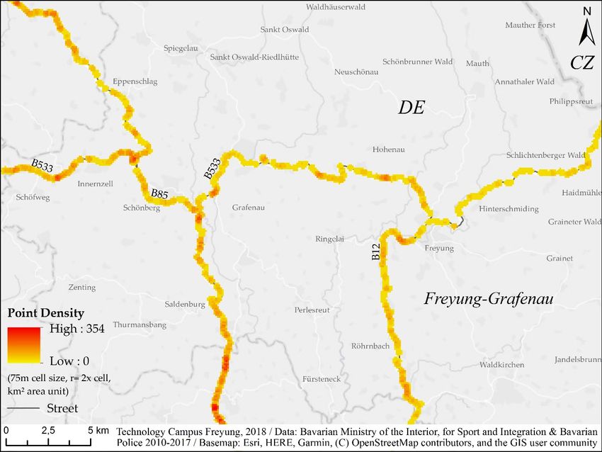
ISPRS Int. J. Geo-Inf. 2019, 8, 66                                                                     2 of 13

computer vision, in combination with GIS-based approaches, would be able to derive a georeferenced
infrastructure inventory from these images. This information could provide knowledge about different
risk types in the road environment, e.g., factors influencing the risk for wildlife crossings.
      Relying on experiences on automatic extraction of road signs from images, (e.g. [4,5]) using artificial
intelligence and machine learning, (e.g. [6,7]), we based our research on the following hypothesis:

(1)    Crash barriers and fences can be identified in a series of inspection images by an artificial neural
       network (ANN).
(2)    Using GIS, a georeferenced inventory of fences and barriers can be built.
(3)    The barriers have a preventive measure while influencing animals’ behavior and, hence,
       reduce accidents.

In this context, we want to especially consider the effect on different species. We restricted the study to
crash barriers and fences, which we will refer to as barriers in the following text.
      At this preliminary research stage, the objective was to test individual steps, which could be
later combined to build an automated process chain from updating the inventory on basis of camera
data through machine learning and GIS-based documentation and analysis. As the majority of
German building authorities only have individual road construction plans with crash barriers and
fences, but not any comprehensive spatial barriers’ documentation available, we propose the machine
learning and GIS-driven approach for automatic identification and georeferencing using existing photo
material from official road inspections. The project is driven by the idea that a better understanding
of animals’ behavior and resulting accidents could help to better plan and place protective measures.
Also, a better warning for car drivers, e.g., through mobile applications, may be a potential opportunity
to increase road security with this combined GIS and machine learning approach.
      In the first part of this paper, we introduce the state of the art in GIS-based WVC analysis,
considering, especially, the aspect of infrastructural effects. Additionally, potential approaches were
analyzed, such as how to integrate ANN for feature detection and GIS to build an infrastructure
inventory. Based on the material of WVCs and images of camera-based road inspections, we developed
a methodology, how to use barriers, derived from computer vision and artificial intelligence in
geospatial modelling. Afterwards, the relation of the occurred WVCs and the presence or absence
of both barrier types is evaluated statistically. After the presentation of our results showing the
species-specific effect, we draw conclusions and propose the next steps to include the abovementioned
results in a larger framework for WVC analysis and prediction.

2. State of Art of GIS-Based WVC Analysis
      Thus far, GIS methods have been utilized by several studies about WVCs to compare the
accident occurrence with environmental, infrastructural, and traffic parameters (e.g., [8]). In order to
contribute to road safety efforts, the GIS studies analyzed WVC development and changes in landscape
structures [9], the placement of warning signs [10], delineating wildlife movement [11], or the impact
of landscape on WVCs [12]. Even though some studies ascertained that infrastructure has an impact
on WVCs [1,13], the number of studies dealing with specific infrastructure types is limited, and those
available are spatially restricted and have not been able to substantially quantify the effect of different
structures, such as barriers and fences, on WVCs [2,14–16]. To the best knowledge of the authors,
until now, no research on the impact of crash barriers has been undertaken at such a scale [14,15].
      For fences, Seiler found out that “Traffic volume, vehicle speed and the occurrence of fences
were dominant factors determining MVC risks” [13] (MVC—moose vehicle collision). While fences
reduce the risk of WVCs, they also seem to shift parts of the risk to the end of the fence [13] and do not
exclude accidents inside the fenced area. As deer, for example, circumvent the fence [17], the collision
risk increases the fence endings by a higher concentration of crossing numbers. Colino-Rabanal et al.
identified in their data that “roadkill was proportionally higher along fenced highways than on similar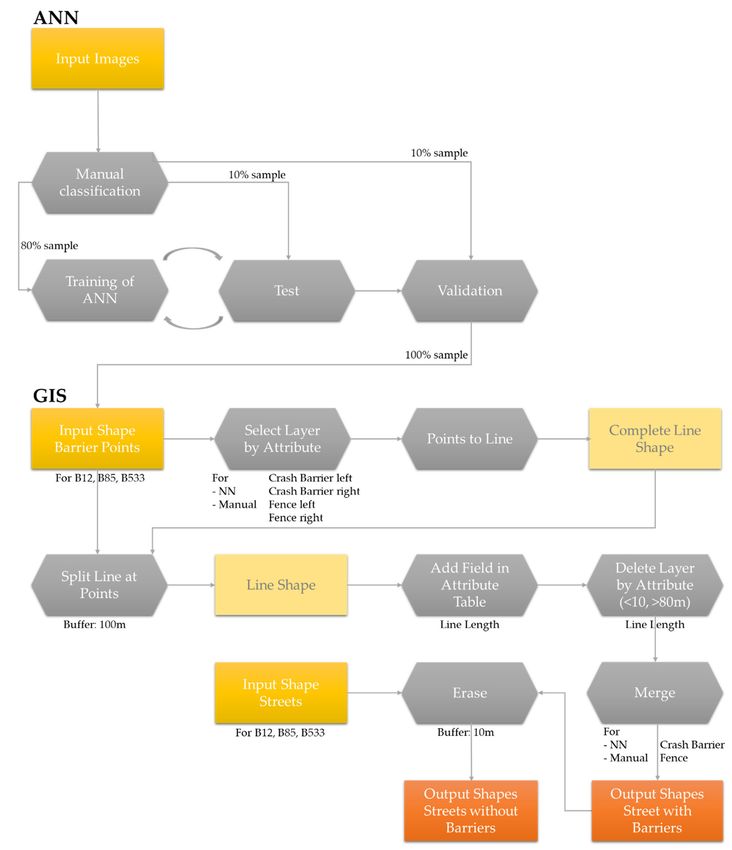
ISPRS Int. J. Geo-Inf. 2019, 8, 66                                                                   3 of 13

major roads that lacked fences” [18], but they mainly see low traffic volumes along these unfenced
roads as the reason for the low numbers of WVCs.
      So far, the availability of data has been restricted and has limited studies from drawing conclusions
about the connection between WVC and infrastructure. Now, camera-based road inspections provide a
huge amount of data to derive inventories from, offering data for the aforementioned limited research
efforts. Therefore, de Frutos et al. suggested to use smartphone-based cameras and apps for video
inspections [19], an alternative option to the more expensive terrestrial laser scanning [20]. Besides,
process chains to collect and evaluate image data using GIS-based handling of camera-based material
and frames have been recommended [21]. The extraction of infrastructure data can be achieved using
computer vision, which was already recommended for camera-based road inspections, but mainly
applied for pavement analysis and road sign detection [22]. The predominant applied example is,
in general, road sign detection [7,23,24], resulting in a vast number of approaches from classical
computer vision [7], via support vector machine [24] and neural networks [6]. The use of artificial
intelligence and neural networks have especially contributed to this domain. While transfer learning
improves the ability to rely on existing nets and focus the learning on specific aspects of a type of
images [25], image databases, such as ImageNet [26,27] and competitions [27,28], contribute to making
the approaches transferrable, systems comparable, and to provide a solid basis for transfer learning.

3. Material and Method
     During the past eight years, Bavarian police recorded all reported WVCs, georeferenced the
location of the accidents, and documented the species of the animal involved in the accident. We used
an excerpt of this dataset for the district of Freyung-Grafenau, a rural accident hotspot in the Bavarian
Forest, Germany (Figure 1). The dataset contains 1571 accidents within the period of 2010–2017 at
secondary roads. As a lot of WVCs occur at overland roads of the secondary street class, we have
chosen a dataset with all three secondary roads B 12, B 85, and B 533 (national roads—Bundesstrasse)
for the analysis. To identify the relevant roadside infrastructure, we used 5596 images recorded
by camera-based inspections along the road, data from official road inspections from the Bavarian
Ministry of the Interior, for Building and Transport of the year 2015. While WVC data covers a period
of the past eight years, the barrier information is, due to the photo material, only a snapshot of the
situation in 2015. However, we assume that the changes in this type of infrastructure are minor and
will not have significant impact on the analysis.
     For the investigation, we used information about animal- and human-preserving barriers (crash
barriers and fences) derived from an automatized image classification with the TensorFlow framework
and a GIS analysis (see Figure 2 for the concept and Figure 3 for the process chain). First, we manually
classified all images of the camera inspection. The basic ANN was constructed by using Inception V3
architecture. For the training, the transfer learning approach was used because the set of available data
was too small to train an own network. A pre-trained network, based on the ImageNet dataset [27],
was taken to support the training work. The output layers were removed, and the network was trained
again, using a set of roughly 800 inspection images.
     Input data to the Inception V3 model are images with a size of 299 × 299 pixels. All input data
was automatically scaled by the TensorFlow framework. Monitoring of the training process showed
that 6000 training steps were sufficient, and further training steps did not increase the classification
quality. Two separate ANNs were used to classify fences and crash barriers. A total of 398 images
was split for fence detection. Manually pre-classified data from the left (211 images) and the right
camera (187 images) were taken, showing fences in comparison to 418 images without fences. For crash
barriers, we used 835 manually pre-classified images with 455 images showing a barrier, and 380
without a barrier. Eighty percent of images were used for training, 10% for validation, and 10% for
testing in the ANN. We shuffled training data to use left and right images alternately.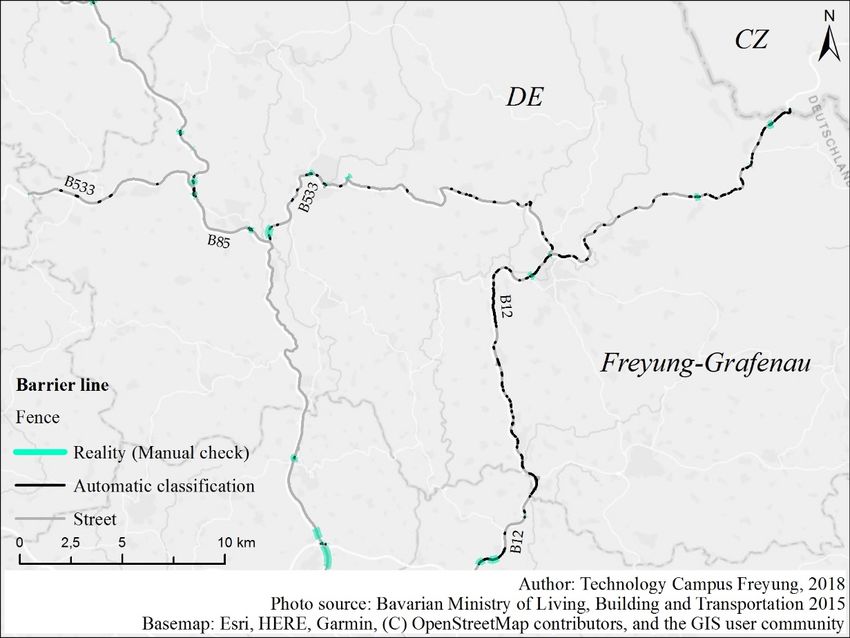
ISPRS Int. J. Geo-Inf. 2019, 8, 66                                                                               4 of 13
   ISPRS Int. J. Geo-Inf. 2018, 7, x FOR PEER REVIEW                                                            4 of 14

ISPRS Int. J. Geo-Inf. 2018, 7, x 1.
                         Figure
                        Figure    FOR PEER REVIEW collision (WVC) density map
                                  1. Wildlife–vehicle
                                     Wildlife–vehicle                     map of
                                                                              of the
                                                                                 the research
                                                                                     research area.
                                                                                              area.            5 of 14

        For the investigation, we used information about animal- and human-preserving barriers (crash
   barriers and fences) derived from an automatized image classification with the TensorFlow
   framework and a GIS analysis (see Figure 2 for the concept and Figure 3 for the process chain). First,
   we manually classified all images of the camera inspection. The basic ANN was constructed by using
   Inception V3 architecture. For the training, the transfer learning approach was used because the set
   of available data was too small to train an own network. A pre-trained network, based on the
   ImageNet dataset [27], was taken to support the training work. The output layers were removed, and
   the network was trained again, using a set of roughly 800 inspection images.

                          Figure 2. 2.
                            Figure  Concept  ofof
                                       Concept  the intersecting
                                                  the            process
                                                      intersecting       forfor
                                                                   process    barriers and
                                                                                barriers   WVC.
                                                                                         and WVC.

      Input   datafirst
        For the     to the  Inception
                        training  of theV3ANN,
                                           model  we are images
                                                       used       withdata
                                                             camera    a size
                                                                           fromof 299
                                                                                  the ×left
                                                                                         299and
                                                                                              pixels.
                                                                                                 rightAll input
                                                                                                       side       data
                                                                                                             of the  car.
was   automatically
  Cameras               scaled by
              were directed     in the
                                   the TensorFlow
                                        front right andframework.
                                                           front leftMonitoring
                                                                      direction. of  the training
                                                                                  While             process
                                                                                           the car was       showed
                                                                                                         permanently
that  6000 at
  driving   training   steps
               the right  sidewere  sufficient,
                               of the            and
                                       street, the     further training
                                                   consequence          steps
                                                                   was that    did
                                                                             the    not increase
                                                                                 distance   betweenthecamera
                                                                                                       classification
                                                                                                               and the
quality.  Two    separate   ANNs    were   used   to  classify fences and  crash  barriers.
  border of the street, where fences are mainly located, was a minimum of 2 to 2.5 m on the  A  total of 398right
                                                                                                              imagesside
was   split for  fence   detection. Manually     pre-classified   data from   the left (211  images)
  (strip of the street plus embankment and drainage system), but at a minimum 5.5 to 6 m at the left  and   the  right
camera (187 images) were taken, showing fences in comparison to 418 images without fences. For
crash barriers, we used 835 manually pre-classified images with 455 images showing a barrier, and
380 without a barrier. Eighty percent of images were used for training, 10% for validation, and 10%
for testing in the ANN. We shuffled training data to use left and right images alternately.
      For the first training of the ANN, we used camera data from the left and right side of the car.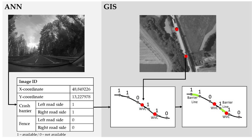
ISPRS Int. J. Geo-Inf. 2019, 8, 66                                                                             5 of 13

 hand side (left lane of the street roughly 3.5 m plus embankment and drainage system). Consequently,
 the images, especially those displaying fences, have different resolutions, due to the distance to the
 camera. Thus, we adapted the methodology later on by only using images from the right side camera
 with a higher resolution of depicted objects for training, resulting in a significantly higher classification
ISPRS Int. J.
 quality,  asGeo-Inf.
              shown   2018,
                        in 7, x FOR PEER
                            Chapter  4. REVIEW                                                         6 of 14

     Figure
      Figure3.3.The
                 Theartificial
                     artificialneural
                                neuralnetwork
                                       network(ANN)
                                               (ANN)and
                                                     andGIS-based
                                                         GIS-basedprocess
                                                                   processtotobuild
                                                                               buildaageoreferenced
                                                                                       georeferencedbarrier
                                                                                                     barrier
      inventoryalong
     inventory    alongroads.
                        roads.

      For further GIS-based
     Approximately             analysis,
                        20 meters   is thethe  image classification
                                           distance    between tworesults
                                                                        imageare   imported
                                                                                points  givinginto ArcGIS (Desktop
                                                                                                information    about
 ArcMap)
the absenceusing  csv format.
              or presence        The result
                            of a fence  and afor   eachbarrier.
                                                crash    image To (identified
                                                                     get linearbyinformation
                                                                                   ID and x and    y coordinates)
                                                                                               about  the length ofis
 separated
both        in four
      barrier       values:
               types,        fence
                       features     present
                                  with   the (1) on the crash
                                              attribute   left road  side, (2)
                                                                  barrier  = 1on(“available”)
                                                                                  the right road  side;
                                                                                                and     crash= barrier
                                                                                                     fence      1 are
 present (3)selected
separately   on the left
                      androad  side, (4)into
                           converted      on the  right
                                             lines.     road points
                                                     Feature    side (see
                                                                       or,Figure
                                                                           rather,2).
                                                                                    image information, which are
classified as non-barrier location, are not considered further. The coordinates of each image point
belong to the original record point, indeed, and not the next few meters visible in the image, where
the barrier may be identified. Nevertheless, the approach is an easy approximation about where a
barrier starts and ends, with a minor uncertainty about the exact start and end point.
     Lines with distances smaller than 10 meters between two single image points were eliminated.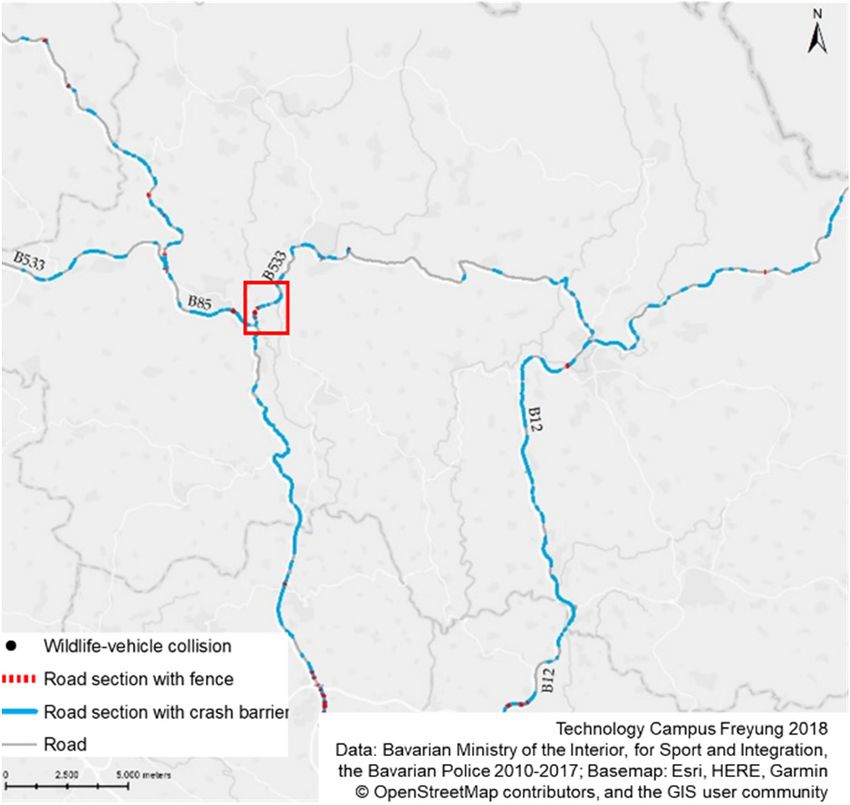
ISPRS Int. J. Geo-Inf. 2019, 8, 66 6 of 13
Approximately 20 m is the distance between two image points giving information about the
absence or presence of a fence and a crash barrier. To get linear information about the length of both
barrier types, features with the attribute crash barrier = 1 (“available”) and fence = 1 are separately
selected and converted into lines. Feature points or, rather, image information, which are classified as
non-barrier location, are not considered further. The coordinates of each image point belong to the
original record point, indeed, and not the next few meters visible in the image, where the barrier may
be identified. Nevertheless, the approach is an easy approximation about where a barrier starts and
ends, with a minor uncertainty about the exact start and end point.
ISPRSLines with 2018,
Int. J. Geo-Inf. distances
7, x FORsmaller than 10 m between two single image points were eliminated.
PEER REVIEW 7 of 14
By testing and comparing with the point information, we found out that 10 m was the minimum for a
(see the casebarrier
reasonable of Figureline,6,deleting
zoom-in map). Instead,
artefacts and veryonly barriers
short lines ofwith more
single thanclassified
wrong two points (longer
images (seethan
the
10
case of Figure 6, zoom-in map). Instead, only barriers with more than two points (longer thanas
meters) were identified. We calculated the Euclidean distance between the points an
10 m)
approximation
were identified.to Wethe road network,
calculated and very
the Euclidean similarbetween
distance to the road line because
the points of the small image
as an approximation to the
points
road network, and very similar to the road line because of the small image points (see also Figurethe
(see also Figure 6). If the distance between two image points was larger than 80 meters, 6).
line
If thewas also eliminated,
distance between two as we assumed
image pointsthat
wasthere is athan
larger gap80in m,
thethe
barrier between
line was also the two points,
eliminated, as weor
two discontinuous
assumed that therepointsis a gap have been
in the connected
barrier by the
between thepoint-in-line
two points, or calculation. As there was
two discontinuous no other
points have
study available for comparison, this threshold is an assumption which was
been connected by the point-in-line calculation. As there was no other study available for comparison, approximated to the real
situation
this thresholdto getisaan realistic
assumption barrier line. was
which Then, the individual
approximated to files for situation
the real left and right
to getside barriersbarrier
a realistic were
merged,
line. Then, the individual files for left and right side barriers were merged, and a new file for the
and a new file for the remaining road sections without barriers was calculated using the
erase function
remaining road(including a 10 m buffer
sections without forwas
barriers lines not lyingusing
calculated exactlytheonerase
the road line (including
function due to inaccurate
a 10 m
GPS
buffer point data).
for lines not Finally, the number
lying exactly on theofroad
WVCslinethat
dueoccurred
to inaccurateon roads with and
GPS point data).without
Finally,barrier lines,
the number
was summed up separately.
of WVCs that occurred on roads with and without barrier lines, was summed up separately.
4. Results
To better discuss
discuss the
the individual
individualparts
partsofofthe
theresearch,
research,we wesplit the
split presentation
the presentationof of
thethe
results in
results
three segments:
in three segments:First, presenting
First, the the
presenting underlying
underlying analysis of WVC
analysis of WVCdata,data,
second, looking
second, at theatGIS-
looking the
based results
GIS-based of barrier
results impact
of barrier on WVCs,
impact andand
on WVCs, third, critically
third, reflect
critically thethe
reflect ANNANNandand
its its
contribution to
contribution
provide the basic infrastructural data.
to provide the basic infrastructural data.
4.1. WVC
WVC Statistics
Statistics
In the district of Freyung-Grafenau,
Freyung-Grafenau, a total of 1571 WVCs occurred on secondary roads in the
years 2010–2017.
2010–2017. The
Theincrease
increaseofofaccidents
accidentsover
overthe past
the eight
past years
eight correlates
years with
correlates the the
with increase of this
increase of
accident
this typetype
accident in Bavaria and and
in Bavaria Germany (Figure
Germany 4). 4).
(Figure
Figure 4. Annual distribution of WVCs (2010–2017).
The WVC distribution by species for the three secondary road sections shows that the vast
majority of accidents is caused by deer, followed by rabbits and foxes (Table 1).
Table 1. The annual distribution of WVCs per species.
Species 2010 2011 2012 2013 2014 2015 2016 2017
Rabbit 8 22 20 15 20 11 20 18ISPRS Int. J. Geo-Inf. 2019, 8, 66 7 of 13
The WVC distribution by species for the three secondary road sections shows that the vast majority
of accidents is caused by deer, followed by rabbits and foxes (Table 1).
Table 1. The annual distribution of WVCs per species.
Species 2010 2011 2012 2013 2014 2015 2016 2017
Rabbit 8 22 20 15 20 11 20 18
Deer 57 151 172 158 136 158 156 182
Other 2 3 3 11 5 8 10 15
Wild Boar 2 0 6 5 1 5 2 9
Fox 3 13
ISPRS Int. J. Geo-Inf. 2018, 7, x FOR PEER REVIEW 13 12 21 17 16 20 8 of 14
Badger 1 7 3 4 2 6 9 11
Wild Bird 2 3 3 1 1 7 2 3
4.2. GIS
4.2. GIS Results
Results
Sixty-four percent
Sixty-four percent ofofroad
roadsegments
segmentsare areaccompanied
accompaniedby bycrash
crashbarriers,
barriers,andandnearly three
nearly three percent
percent of
roads
of areare
roads protected
protected by by
fences, as Figure
fences, 5 shows
as Figure 5 shows forfor
thethe
whole research
whole areaarea
research (a),(a),
andand
for for
oneone section (b).
section
In Tables 2 and 3, we compared the dependencies between WVCs, barriers,
(b). In Table 2 and 3, we compared the dependencies between WVCs, barriers, and fences for the and fences for the manual
and ANN-based
manual classification.
and ANN-based The comparison
classification. of WVCs with
The comparison of areas
WVCsprotected
with areas by crash barriers
protected byresults
crash
in an equal number of the total 1571 accidents that happened in sections with
barriers results in an equal number of the total 1571 accidents that happened in sections with barriersbarriers (776) versus
the accidents
(776) versus the in areas without
accidents barriers
in areas (795).
without Due to(795).
barriers the high
Dueclassification quality, the manual
to the high classification quality,and the
automatic
manual andclassification
automatic provided similar
classification results.similar
provided By considering
results. the
By length of the the
considering sections
length withof and
the
without barriers,
sections with andthe number
without of WVCs
barriers, theper lengthof
number is WVCs
2.11 times
per higher
lengthin is sections
2.11 times without
highercrash barrier
in sections
(3.30 times higher using ANN classification) in comparison to sections without
without crash barrier (3.30 times higher using ANN classification) in comparison to sections without barriers or, the other
way around,
barriers or, thethe street
other waysection where
around, one when
the street WVC
section occurs
where one is 2.11WVC
when timesoccurs
longerison average
2.11 (WVC
times longer
proportion to street length).
on average (WVC proportion to street length).
(a) (b)
Figure 5. Spatial distribution of barriers in the research area (a) and in a subsection (b).
Figure 5. Spatial distribution of barriers in the research area (a) and in a subsection (b).
The distribution of WVCs shows that barriers have an impact on accidents. Especially crash
The distribution of WVCs shows that barriers have an impact on accidents. Especially crash
barriers seem to significantly influence the accident situation for all animals, particularly on special
barriers seem to significantly influence the accident situation for all animals, particularly on special
species (see also Table 4). The impact of fences on WVCs needs to be discussed because current data
species (see also Table 4). The impact of fences on WVCs needs to be discussed because current data
would support the hypothesis that fences would increase the risk of WVCs by the factor 3.08, or areas
would support the hypothesis that fences would increase the risk of WVCs by the factor 3.08, or areas
without fences would have 0.32 times lower risk of accidents. For a total of 113 km, we identified less
than 3 km of fenced road segments.ISPRS Int. J. Geo-Inf. 2019, 8, 66 8 of 13
without fences would have 0.32 times lower risk of accidents. For a total of 113 km, we identified less
than 3 km of fenced road segments.
Table 2. Results of WVC numbers at roads with and without crash barriers for the road segments
identified by ANN in comparison to the manual classification.
Total Number
Crash Barriers Neural Network Manual Check
of WVC
With Without With Without
Barrier Barrier Barrier Barrier
Number of WVC 1571 776 795 720 851
(%) (100%) (49.40%) (50.60%) (45.83%) (54.17%)
Street length (km) 86.257 26.746 72.489 40.514
Street Length / WVC 111.16 33.64 100.68 47.61
WVC Proportion to Street Length 3.30 0.30 2.11 0.47
Table 3. Results of WVC numbers at roads with and without fences for the road segments identified by
ANN in comparison to the manual classification.
Total Number
Fences Neural Network Manual Check
of WVC
With Without With Without
Fence Fence Fence Fence
Number of WVC 1571 211 1360 109 1462
(%) (100%) (13.43%) (86.57%) (6.94%) (93.06%)
Street length (km) 5.429 107.574 2.668 110.335
Street Length/ WVC 25.73 79.10 24.48 75.47
WVC Proportion to Street Length 0.33 3.07 0.32 3.08
The hypothesis that animals will circumvent the fence and the number of WVCs will increase at
the end of a fenced section is supported by literature [17], and would help to better understand the
statistical result. For short fenced sections, also, the inaccuracies in fence positions as well as accident
positions may support this theory, because some of the accidents, marked as inside the fenced road
section, may have been located near the end of the fence, and could be explained by circumventing.
The effect of crash barriers and fences also depends on the species. Crash barriers seem to have an
even stronger retaining effect on badgers and foxes but, also, for the predominant deer population in
the area, street segments without crash barriers have a two-times higher (2.16) probability for accidents
in comparison to segments with crash barrier (Table 4). The numbers for rabbits indicate that especially
smaller animals, such as rabbits and “others”, seem not to be retained by fences at all. The two-times
higher probability for wild birds may explain that the effect on other species might affect the behavior
to search for carcasses.
Table 4. WVC per species proportional to street length for road segments with crash barriers and fences.
WVC Proportion to Street Length
Species Crash Barrier Fence
Rabbit 2.57 0.25
Deer 2.16 0.34
Other 1.61 0.21
Wild Boar 2.68 0.34
Fox 3.35 0.32
Badger 4.13 0.50
Wild Bird 2.15 0.51
All species 2.11 0.32ISPRS Int. J. Geo-Inf. 2019, 8, 66 9 of 13
We did not distinguish between different fence types (game fence, non-permanent pasture fence,
smaller barriers, and garden fences). Different types might retain some species and may have no effect
on others.
ISPRS Also, 2018,
Int. J. Geo-Inf. the length
7, x FORofPEER
fenced segments should be further analyzed as circumventing may
REVIEW play
10 of 14
a role for wildlife crossings and for the WVC risk. For further research, even larger datasets and a
better classification of fences will be Deer
necessary. 2.16 0.34
The large dataset of WVCs is Other 1.61monitoring
a result of a long 0.21
period (eight years), while barrier
data only represents a temporal Wild Boar from 2015.
snapshot 2.68 As a consequence,
0.34 also, more time frames of
Fox 3.35
infrastructure are necessary to analyze changes of constructions. 0.32
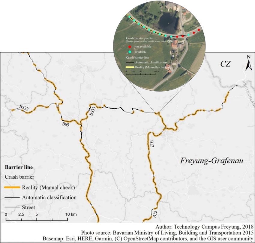
Figure 6 (for crash barriers) and Badger 4.13 are the resulting
Figure 7 (for fences) 0.50 maps with the georeferenced
barrier inventory. The comparison Wild ofBird 2.15 classification
the automatized 0.51 with the manually checked road
sections shows a high correspondence All species 2.11identification
of crash barrier 0.32 and the improving requirements
in the case of the fence digitization. The small zoom-in map of Figure 6 presents the advantage of the
ANNThe andlargeGIS combination,
dataset of WVCs as the
is share of correct
a result identified
of a long road period
monitoring sections(eight
are increased by using
years), while the
barrier
GIS approach.
data only represents However, it also shows
a temporal snapshot thatfrom
the accuracy
2015. Asofa the automatic also,
consequence, classification
more timestillframes
needs of
to
be improved. are necessary to analyze changes of constructions.
infrastructure
Figure
Figure 6.
6. Map of classified
Map of classifiedcrash
crashbarriers
barriers(black
(black line)
line) in in comparison
comparison to reality
to reality (manual
(manual check,
check, orange
orange line).
line).ISPRS Int. J. Geo-Inf. 2019, 8, 66 10 of 13
ISPRS Int. J. Geo-Inf. 2018, 7, x FOR PEER REVIEW 11 of 14
Figure 7. Map of classified fences (black line) in comparison to reality (manual check, turquoise line).
4.3. ANN
FigureResults
6 (for crash barriers) and Figure 7 (for fences) are the resulting maps with the
georeferenced barrier inventory.
The auto-classification by ANN Theresulted
comparison of theclassification
in a 92% automatizedrateclassification
to identify with
crashthe manually
barriers and
checked
a 63% rateroad
for sections shows
fences (Table 5).aIn
high correspondence
particular, of crash barrier
the low classification identification
quality and result
of fences may the improving
from the
requirements
fragile structurein of
the case in
fences of combination
the fence digitization. The small
with the differing zoom-in
resolution of map
imagesof from
Figurethe6 two
presents the
different
advantage of the ANN and GIS combination, as the share of correct identified
cameras. We later analyzed this difference in resolution by first training the ANN with images fromroad sections are
increased
both sides by
and,using the with
second, GIS approach.
images onlyHowever,
from theitright
also side,
shows andthat thethis
used accuracy
trainedofANNthe automatic
to classify
classification still needs to be
images from both sides of the road. improved.
4.3. ANN Results Table 5. Quality of auto-classification of images by the ANN.
The auto-classification
Barrier Left by ANN
Barrier resulted
Right in a 92%
Barrier Totalclassification
Fence Leftrate to identify
Fence Rightcrash barriers
Fence Totaland
a 63% rate for fences (Table 5). In particular, the low classification quality of fences may result from
False 7.72% 7.70% 7.71% 55.25 19.50% 37.37%
the fragile
True structure
92.28%of fences 92.30%
in combination92.29%
with the differing
44.75%resolution of images from
80.50% the two
62.63%
different cameras. We later analyzed this difference in resolution by first training the ANN with
images from both sides and, second, with images only from the right side, and used this trained ANN
Results (Table 6) show that training data stemming from both cameras results in a significant
to classify images from both sides of the road.
larger number of misclassifications. Training the ANN only with camera data from the right side
resulted in nearly 8% more correct positives (ANN identified fences, where fences are on the image) as
Table 5: Quality of auto-classification of images by the ANN.
well as 12% more correct negative (ANN identified no fence, where no fences are). This may indicate
Barrier Barrier Barrier Fence Fence Fence total
that for slim structures, such as fences, resolution is a key aspect for training that will also result in
left right total left right
positive classification results for images with a lower resolution of the object.
False 7.72% 7.70% 7.71% 55.25 19.50% 37.37%
The classification results for crash barriers are significantly better than those for fences. Crash
True 92.28% 92.30% 92.29% 44.75% 80.50% 62.63%
barriers are, in general, located closer to the road and provide larger and more significant structures.
Fences are often located behind crash barriers or even far from the street, which means that fences are
below Results (Tablethat
a resolution 6) show
couldthat trainingby
be detected data
ANN,stemming from
or can be bothupcameras
mixed with slim results in a significant
and elongate bushes
larger number of misclassifications. Training
and small trees, such as birches or hazelnut. the ANN only with camera data from the right side
resulted in nearly 8% more correct positives (ANN identified fences, where fences are on the image)
as well as 12% more correct negative (ANN identified no fence, where no fences are). This mayISPRS Int. J. Geo-Inf. 2019, 8, 66 11 of 13
Table 6. Comparison of automatic image recognition using neural network with training of images of
both sides and only right side and the relative change.
Training on Images Relative Change
Of Both Sides Of Only Right Side
Fence No Fence Fence No Fence Fence No Fence
Correct 142 3507 153 3943 7.75% 12.43%
Right
False 1837 105 1398 97 −23.90% −7.62%
Correct 147 2064 166 2699 12.93% 30.77%
Left
False 3343 37 2695 31 −19.38% −16.22%
Subsequently we can summarize that pre-trained ANN can be used through transfer learning to
identify barriers and fences as roadside infrastructure and create an inventory using GIS techniques,
building up an inventory and analyzing the occurrence and cause effect relationships between
infrastructure and WVC. Image resolution and the size of the dataset are essential factors for
the analysis.
5. Conclusions
In this study, we analyzed the impact of barriers (crash barriers and fences) on the risk of
WVCs. We followed the hypothesis that (1) crash barriers and fences can be identified in a series of
camera-based road inspection images by an ANN and that (2) a georeferenced inventory of fences and
barriers can be built using GIS. Based on this data, we found a preliminary answer to the question
of up to which extent barriers can have a preventive measure while influencing animals’ behavior to
reduce accidents and increase safety. While a barrier effect of crash barriers is visible, fence impacts
must be researched more precisely in the next step. Using ANN to identify barriers in the images
provided, in a first attempt, already adequate results, sufficient to delineate barriers in a GIS. GIS was
in this part able not only to build the polylines of these structures but also to compensate errors of the
ANN by restricting results to a spatially reasonable dataset.
Due to these new possibilities to derive the location and extent of road-accompanying barriers
from camera images, we were able to compare, in a preliminary study, 113 km of road network with
WVCs from an eight-year period. We found that crash barriers have a strong effect on wildlife and,
thus, reduce the risk of WVCs by one-half. For our test site, fences seem not to affect animals, but this
requires further testing with a larger region and an increased number of roadside fences. However, the
crash barrier information can already be considered in a new type of WVC warning system for car
drivers to better predict areas at risk, or to improve planning of protection measures.
From a methodological perspective, the combination of artificial intelligence with GIS provides a
new concept to make a study on a topic, where up-to-date quantitative research was not possible due to
a lack of data. The study still leaves some questions open and requires further consideration to improve
the quality of results as well as the accuracy of geodata with regard to completeness and precision
of location. The classification of fences needs to be developed further due to different fence types,
having differing visual appearance and effects on wildlife. There is a need to distinguish between
game fences, protection fences, as well as garden fences, and other possible subtypes. For this new
training material and, also, a larger test region, it will be necessary to increase the total available length
of fences and sections for different fence types. Additionally, the resolution of the inspection images
might contribute to a better quality of the ANN’s detection rate. We applied a standard resolution of
299 × 299 pixels to use an existing trained network for transfer learning. Using the available image
resolution and training an own neural network will increase the effort to manually classify sufficient
data but might also improve barrier—especially fence—recognition.
From a data perspective, three aspects should be considered in the future: (1) Infrastructure
developments over time. The length of the available time series (eight years for WVC) will require
consideration of the development of the built environment at and along a street in the future. This willISPRS Int. J. Geo-Inf. 2019, 8, 66 12 of 13
increase complexity from a GIS perspective, to take into account spatiotemporal data. The problem
is, again, data availability due to missing documentation of these structures. While accidents are
documented on a daily basis, changes of infrastructure might be only considered depending on
inspection intervals. (2) Other types of barriers, such as noise protection barriers, dams, and hill
intersections with steep slopes, walls, or gullies were not considered in this study, but might also
impact animals’ behavior and movement patterns and, hence, WVC occurrence and risk. These types
of structures are also undocumented and can only partially be derived from photos. Mixed approaches,
combining inspection images and laser scanning data, might provide the necessary information. Then,
the presented methodology might be applied to these infrastructure types. (3) While past studies
only considered a small number of WVC-influencing factors, the current study and its applicability
to alternative barrier types indicates that a significant number of parameters needs to be considered
to explain WVC development. Besides road infrastructure and traffic as WVC-influencing factors,
a better understanding of habitats and wildlife behavior will also be necessary.
Approaches from artificial intelligence and big data might be used to better process these
heterogeneous datasets and consider a larger set of potentially influencing parameters. In the future,
results might be used for more effective warning of car drivers, substituting warning signs by more
precise spatial and temporal and, hence, highly dynamic warnings. To increase road safety in general,
this approach might also be applied to other types of accidents.
Author Contributions: Conceptualization, R.P. and W.D.; methodology, R.P., W.D.; validation/formal
analysis/investigation, R.P.; writing, W.D. and R.P.; visualization, R.P.; supervision, W.D.
Funding: This research was funded by the GERMAN FEDERAL MINISTRY OF TRANSPORT AND DIGITAL
INFRASTRUCTURE (BMVI) as part of the mFund project “WilDa—Dynamic Wildlife–vehicle collision warning,
using heterogeneous traffic, accident and environmental data as well as big data concepts” grant number 19F2014A.
Acknowledgments: Accident data provided by the Bavarian Ministry of the Interior, for Sport and Integration
and the Bavarian Police; photo material provided by Bavarian Ministry of Living, Building and Transportation.
Conflicts of Interest: The funders had no role in the design of the study; in the collection, analyses, or
interpretation of data; in the writing of the manuscript, or in the decision to publish the results.
References
1. Seiler, A. Predicting locations of moose-vehicle collisions in Sweden. J. Appl. Ecol. 2005, 42, 371–382.
[CrossRef]
2. Malo, J.E.; Suárez, F.; Díez, A. Can we mitigate animal–vehicle accidents using predictive models? J. Appl. Ecol.
2004, 41, 701–710. [CrossRef]
3. Gunson, K.E.; Mountrakis, G.; Quackenbush, L.J. Spatial wildlife-vehicle collision models: A review of
current work and its application to transportation mitigation projects. J. Environ. Manag. 2011, 92, 1074–1082.
[CrossRef] [PubMed]
4. Fang, C.-Y.; Chen, S.-W.; Fuh, C.-S. Road-sign detection and tracking. IEEE Trans. Veh. Technol. 2003,
52, 1329–1341. [CrossRef]
5. Khan, J.F.; Bhuiyan, S.M.A.; Adhami, R.R. Image Segmentation and Shape Analysis for Road-Sign Detection.
IEEE Trans. Intell. Transp. Syst. 2011, 12, 83–96. [CrossRef]
6. Kellmeyer, D.L.; Zwahlen, H.T. Detection of highway warning signs in natural video images using color
image processing and neural networks. In Proceedings of the 1994 IEEE International Conference on Neural
Networks (ICNN’94), Orlando, FL, USA, 28 June–2 July 1994; Volume 7, pp. 4226–4231.
7. Ouerhani, Y.; Elbouz, M.; Alfalou, A.; Kaddah, W.; Desthieux, M. Road sign identification and geolocation
using JTC and VIAPIX module. Proc. SPIE 2018, 10649, 106490J. [CrossRef]
8. Pagany, R.; Dorner, W. Spatiotemporal analysis for wildlife-vehicle-collisions based on accident statistics of
the county Straubing-Bogen in Lower Bavaria. ISPRS Int. Arch. Photogramm. Remote Sens. Spat. Inf. Sci. 2016,
XLI-B8, 739–745. [CrossRef]
9. Keken, Z.; Kušta, T.; Langer, P.; Skaloš, J. Landscape structural changes between 1950 and 2012 and their role
in wildlife–vehicle collisions in the Czech Republic. Land Use Policy 2016, 59, 543–556. [CrossRef]ISPRS Int. J. Geo-Inf. 2019, 8, 66 13 of 13
10. Krisp, J.M.; Durot, S. Segmentation of lines based on point densities—An optimisation of wildlife warning
sign placement in southern Finland. Accid. Anal. Prev. 2007, 39, 38–46. [CrossRef]
11. Nelson, T.; Long, J.; Laberee, K.; Stewart, B. A time geographic approach for delineating areas of sustained
wildlife use. Ann. GIS 2015, 21, 81–90. [CrossRef]
12. Nielsen, C.K.; Anderson, R.G.; Grund, M.D. Landscape Influences on Deer-Vehicle Accident Areas in an
Urban Environment. J. Wildl. Manag. 2003, 67, 46–51. [CrossRef]
13. Oskinis, V.; Ignatavicius, G.; Vilutiene, V. An evaluation of wildlife-vehicle collision pattern and associated
mitigation strategies in Lithuania. Environ. Eng. Manag. J. 2013, 12, 2323–2330.
14. Clevenger, A.P.; Kociolek, A.V. Potential impacts of highway median barriers on wildlife: State of the practice
and gap analysis. Environ. Manag. 2013, 52, 1299–1312. [CrossRef] [PubMed]
15. Kociolek, A.; Clevenger, A.P. Highway median Impacts on Wildlife Movement and Mortality. In Proceedings
of the 2007 International Conference on Ecology & Transportation “Bridging the Gaps, Naturally”
(ICOET 2007), Little Rock, AR, USA, 20–25 May 2007.
16. Boarman, W.I.; Sazaki, M.; Jennings, W.B. The Effect of Roads, Barrier Fences, and Culverts on Desert Tortoise
Populations in California. In Proceedings of the Conservation, Restoration, and Management of Tortoises
and Turtles—An International Conference, New York, NY, USA, 11–16 July 1993; pp. 54–58.
17. Gulsby, W.D.; Stull, D.W.; Gallagher, G.R.; Osborn, D.A.; Warren, R.J.; Miller, K.V.; Tannenbaum, L.V.
Movements and home ranges of white-tailed deer in response to roadside fences. Wildl. Soc. Bull. 2011,
35, 282–290. [CrossRef]
18. Colino-Rabanal, V.J.; Lizana, M.; Peris, S.J. Factors influencing wolf Canis lupus roadkills in Northwest Spain.
Eur. J. Wildl. Res. 2011, 57, 399–409. [CrossRef]
19. Higuera de Frutos, S.; Castro, M. Using smartphones as a very low-cost tool for road inventories. Transp. Res.
Part C Emerg. Technol. 2014, 38, 136–145. [CrossRef]
20. Gong, J.; Zhou, H.; Gordon, C.; Jalayer, M. Mobile Terrestrial Laser Scanning for Highway Inventory Data
Collection. Comput. Civ. Eng. 2012. [CrossRef]
21. Khan, G.; Santiago-Chaparro, K.R.; Chiturri, M.; Noyce, D.A. Development of Data Collection and Integration
Framework for Road Inventory Data. Transp. Res. Rec. 2010, 2160, 29–39. [CrossRef]
22. Varadharajan, S.; Jose, S.; Sharma, K.; Wander, L.; Mertz, C. Vision for road inspection. In Proceedings of the
IEEE Winter Conference on Applications of Computer Vision, Steamboat Springs, CO, USA, 24–26 March
2014; pp. 115–122.
23. de la Escalera, A.; Moreno, L.E.; Salichs, M.A.; Armingol, J.M. Road traffic sign detection and classification.
IEEE Trans. Ind. Electron. 1997, 44, 848–859. [CrossRef]
24. Greenhalgh, J.; Mirmehdi, M. Real-Time Detection and Recognition of Road Traffic Signs. IEEE Trans. Intell.
Transp. Syst. 2012, 13, 1498–1506. [CrossRef]
25. Lagunas, M.; Garces, E. Transfer Learning for Illustration Classification. arXiv 2018, arXiv:1806.02682.
26. Krizhevsky, A.; Sutskever, I.; Hinton, G.E. ImageNet classification with deep convolutional neural networks.
Commun. ACM 2017, 60, 84–90. [CrossRef]
27. Russakovsky, O.; Deng, J.; Su, H.; Krause, J.; Satheesh, S.; Ma, S.; Huang, Z.; Karpathy, A.; Khosla, A.;
Bernstein, M.; et al. ImageNet Large Scale Visual Recognition Challenge. Int. J. Comput. Vis. 2015,
115, 211–252. [CrossRef]
28. Houben, S.; Stallkamp, J.; Salmen, J.; Schlipsing, M.; Igel, C. Detection of traffic signs in real-world images:
The German traffic sign detection benchmark. In Proceedings of the 2013 International Joint Conference on
Neural Networks (IJCNN), Dallas, TX, USA, 4–9 August 2013; pp. 1–8.
© 2019 by the authors. Licensee MDPI, Basel, Switzerland. This article is an open access
article distributed under the terms and conditions of the Creative Commons Attribution
(CC BY) license (http://creativecommons.org/licenses/by/4.0/).You can also read