Color Variants Identification in Fashion e-commerce via Contrastive Self-Supervised Representation Learning
←
→
Page content transcription
If your browser does not render page correctly, please read the page content below
Color Variants Identification in Fashion e-commerce via
                                                               Contrastive Self-Supervised Representation Learning
                                                          Ujjal Kr Dutta , Sandeep Repakula , Maulik Parmar and Abhinav Ravi
                                                                             Data Sciences-Image Sciences, Myntra
                                                                                  Bengaluru, Karnataka, India
                                                                  {ujjal.dutta,sandeep.r,parmar.m,abhinav.ravi}@myntra.com
arXiv:2104.08581v2 [cs.CV] 30 Jun 2021

                                                                   Abstract
                                              In this paper, we utilize deep visual Representation
                                              Learning to address an important problem in fashion
                                              e-commerce: color variants identification, i.e., iden-
                                              tifying fashion products that match exactly in their
                                              design (or style), but only to differ in their color. At
                                                                                                                                 Anchor         Positive          Negative
                                              first we attempt to tackle the problem by obtaining
                                                                                                                                   ( Color Variants )      ( Not Color Variant )
                                              manual annotations (depicting whether two prod-
                                              ucts are color variants), and train a supervised triplet       Figure 1: Illustration of the color variants identification problem.
                                              loss based neural network model to learn representa-           The anchor and positive images contain fashion products that have
                                                                                                             the exact same design/ style, but different colors (anchor is blue, and
                                              tions of fashion products. However, for large scale            positive is black). The negative image contains a product that is not
                                              real-world industrial datasets such as addressed in            a color variant to the anchor and the positive. NOTE: The images
                                              our paper, it is infeasible to obtain annotations for          belong to www.myntra.com.
                                              the entire dataset, while capturing all the difficult
                                                                                                             each other. These class labels are used to obtain triplet
                                              corner cases. Interestingly, we observed that color
                                                                                                             based constraints, consisting of an anchor, a positive and
                                              variants are essentially manifestations of color jit-
                                                                                                             a negative (Figure 1). The positive is usually an image
                                              ter based augmentations. Thus, we instead explore
                                                                                                             that consists of a product that is a color variant of the
                                              Self-Supervised Learning (SSL) to solve this prob-
                                                                                                             product contained in the anchor image. The negative is
                                              lem. We observed that existing state-of-the-art SSL
                                                                                                             an image that consists of a product that is not a color
                                              methods perform poor, for our problem. To address
                                                                                                             variant of the products contained in the anchor and posi-
                                              this, we propose a novel SSL based color variants
                                                                                                             tive images. These triplets are used to train a supervised
                                              model that simultaneously focuses on different parts
                                                                                                             triplet loss based neural network model [Schroff et al., 2015;
                                              of an apparel. Quantitative and qualitative evalu-
                                                                                                             Veit et al., 2017] in order to obtain deep embeddings of fash-
                                              ation shows that our method outperforms existing
                                                                                                             ion products. Having obtained the embeddings, we perform
                                              SSL methods, and at times, the supervised model.
                                                                                                             clustering on them to group the color variants.
                                                                                                                A key challenge in this supervised approach is that of ob-
                                         1   Introduction                                                    taining manual annotations, which not only requires fashion
                                         In this paper, we address a very crucial problem in fashion         domain expertise, but is also infeasible, given the large scale
                                         e-commerce, namely, automated color variants identification,        of our platform, and the huge number and complexity of the
                                         i.e., identifying fashion products that match exactly in their      fashion products. As visual Self-Supervised Learning (SSL)
                                         design (or style), but only to differ in their color (Figure 1).    obtains image embeddings without requiring manual annota-
                                         Our motivation to pick the use-case of color variants identifica-   tions, we consider it as a candidate to address our problem,
                                         tion for fashion products comes from the following reasons: i)      i.e., lack of annotations for our large data. The motivation
                                         Fashion products top across all categories in online retail sales   for this comes from the fact that typcial visual SSL methods
                                         [Jagadeesh et al., 2014], ii) Most often users hesitate to buy a    employ a color jitter based data augmentation step.
                                         fashion product solely due to its color despite liking all other       Interestingly, color variants of fashion products are in
                                         aspects of it. Providing more color options increases add-to-       essence, manifestations of color jittering. It should be noted
                                         cart ratio, thereby generating more revenue, along with im-         that a Product Display Page (PDP) image in a fashion e-
                                         proved customer experience. At Myntra (www.myntra.com),             commerce platform may contain multiple fashion products.
                                         a leading e-commerce platform, we address this problem by           Thus, we must apply an object detector to localise our primary
                                         leveraging deep visual Representation/Embedding Learning.           fashion product of interest (Figure 3). However, when we
                                            Firstly, we obtained manual annotations (class labels) in-       already employ object detection, the standard random crop
                                         dicating whether two product images are color variants to           step used in existing SSL methods may actually miss out im-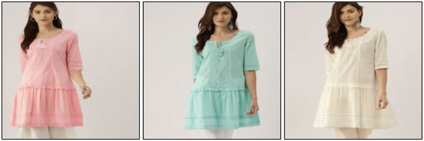
Anchor (A)   Positive (P)                              Negative (N)

                                     A model trained to
                                     group together
                                     Crop_A and Crop_P
                                                                                                                                                         Cluster 2
                                     might incorrectly learn                                                                                Cluster 1
                                     to group Crop_N
                                     along with Crop_A                                                             Embedding
                                                                                             Object
                                                                                                                   Learning
                                     and Crop_P, because                                     Detector
                                                                                                                   Model
                                     all three crops are
                                     visually very “similar”.                                Step 1                  Step 2
                                                                                                                                               Step 3:

                                     Thus, a single random                                                                                     Clustering in
                                     crop may not be                                                                                           Embedding
                                     sufficient to represent                                                                                   Space
                                     an entire image for                                                Training               Embeddings
                                     the purpose of                                                     Triplets
                                     forming contrastive
                                     pairs.
                                                                               Figure 3: Proposed pipeline to address the color variants identification
          Crop_A        Crop_P                                    Crop_N       problem by using a supervised embedding learning model.
Figure 2: Drawbacks of using random crop to form contrastive pairs                Visual SSL [Jing and Tian, 2020] refers to the learning of
in our use-case.                                                               representations of images without making use of class labels.
portant regions of a fashion product, which might be crucial                   A popular paradigm of SSL is contrastive learning, that groups
in identifying color variants (Figure 2).                                      together embeddings obtained from augmentations of the same
   For this reason, we rather choose to propose a novel SSL                    image. Many recent SSL approaches have been proposed
variation that considers multiple slices/ patches of the primary               that vary in their implementation details (for example, using
fashion object (after object detection), and simultaneously                    momentum encoding, memory module, only positive pairs,
obtains embeddings for each of them. The final sum-pooled                      etc) [Chen et al., 2020; He et al., 2020; Grill et al., 2020;
embedding is then used to optimize a SSL based contrastive                     Chen and He, 2021].
loss (Figure 4). We call our method as Patch-Based Con-
trastive Net (PBCNet). We conjecture that considering mul-
tiple patches i) do not leave things to chance (as in random
                                                                               3     Proposed Approach
crops), and provides a deterministic approach to obtain em-                    In this section, we discuss the Representation Learning meth-
beddings, ii) enables us to borrow more information (from                      ods used to address the problem of color variants identification.
other patches) to make a better decision on grouping a pair
of similar embeddings. Our conjecture is supported not only                    3.1    Supervised Color Variants Model
by evidence of improved discriminative performances by the                     Firstly, we shall discuss the proposed supervised approach of
consideration of multiple fine patches of images [Wang et al.,                 addressing the color variants identification problem. Our pro-
2018], but also by our experimental results, where our method                  posed pipeline leveraging the supervised model is illustrated
consistently outperforms existing SSL methods on our task,                     in Figure 3. The pipeline consists of the following major com-
and also the supervised baseline.                                              ponents (or steps) in the same order: i) Object Detection, ii)
   Following are the major contributions of the paper:                         Embedding Learning and iii) Clustering. As the original input
  1. A supervised triplet loss based visual Representation                     image usually consists of a human model wearing secondary
      Learning approach to identify color variants among fash-                 fashion products as well, we perform object detection to lo-
      ion products (to the best of our knowledge addressed for                 calise the primary fashion product of interest. Having obtained
      the first time).                                                         the cropped image of the fashion article, we form triplet based
  2. A systematic study of existing state-of-the-art SSL meth-                 constraints (in the form of anchor, positive and negative) using
      ods to solve the proposed problem while alleviating the                  the available manual annotations. These triplets are used to
      need for manual annotations.                                             train an embedding learning model. The obtained embeddings
  3. A novel contrastive loss based SSL method that focuses                    are then grouped together by using an appropriate clustering
      on parts of an object to identify color variants.                        algorithm. An obtained cluster then contains embeddings of
                                                                               images of fashion products that are color variants to each other.
                                                                                  However, the supervised model needs manual annotations
2   Related Work                                                               which may be infeasible to obtain in large real-world industrial
The problem of visual embedding/ metric learning refers to                     datasets (such as those present in our platform). Thus, we
that of obtaining vector representations/embeddings of images                  now propose a novel self-supervised representation learning
in a way that the embeddings of similar images are grouped to-                 model to identify color variants without making use of manual
gether while moving away dissimilar ones. Several approaches                   annotations.
have been proposed in the recent literature, which can be cate-
gorized as either supervised [Sun et al., 2020; Levi et al., 2020;             3.2    Self-Supervised Color Variants Model
Gu and Ko, 2020] or unsupervised [Dutta et al., 2020b;                         As discussed using Figure 2, a random crop of an image may
Cao et al., 2019; Li et al., 2020; Dutta et al., 2020a]. Typically,            not be the best representative to form contrastive pairs for
a key aspect of such approaches is that of providing constraints               SSL, at least for our task. Hence, we propose a method that
for optimizing a suitable objective function. Popular forms                    simultaneously considers multiple, fixed, slices/patches of an
of constraints in embedding learning are either in the form                    object to form embeddings. This is illustrated in Figure 4. As
of pairs, triplets or tuples, that indicate embeddings of which                our contribution is only specific to the embedding learning
examples need to be brought closer.                                            component, Figure 4 focuses only on this. As illustrated, the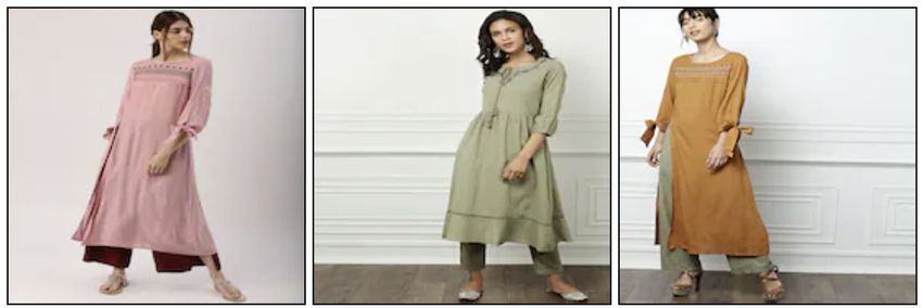
of the memory module. Our method is called as Patch-Based
                                                 Left Embedding                       Contrastive Net (PBCNet).

                                                      Right Embedding
                                                                                      4     Experiments
                Left Slice
                                                                                      We evaluated the discussed methods on a large (orders of
                                   Right Slice    Embedding
                                                  Learning                            magnitudes of 105 ) internal collection of challenging real-
                                                  Model
                                                                                      world industrial images on our Myntra platform (www.myntra.
                                                                            Final
                     Top Slice                       Top Embedding        Embedding   com) that hosts various fashion products. In this section, we
     Original
                                                                                      report our results on a collection of roughly2 0.13 million
     Cropped
     Image
                                                                                      Kurtas images from our internal database. We used the exact
                                                       Bottom Embedding
                                                                                      same set to train the supervised (with labeled training data)
                    Bottom Slice
        Figure 4: Illustration of our slicing based approach.
                                                                                      and self-supervised methods (without labeled training data)
multiple patches of an object are obtained by performing slices                       for a fair comparison. For inferencing, we used the entire
of the image to obtain the left, right, top and bottom views of                       0.13 million Kurtas images, which are present in the form of
the object under consideration. We then pass each of these                            different dataset splits (based on brand, gender, MRP). We
slices through the base encoder of the embedding learning                             refer to our 6 dataset splits as Data 1-6. Details of the data
model to obtain four different embeddings, which are then                             and the performance metrics (CGacc for all splits, ARI, FMS
added1 to obtain the final representation of the object.                              and CScore for splits 4-6, a higher value indicates a better
   We make use of negative pairs in our method because we                             performance) are deferred to the supplementary material.
found the performance of methods that do not make use of                                 Methods Compared: Following are the methods that we
negative pairs (eg, SimSiam [Chen and He, 2021], BYOL                                 have compared for representation learning:
[Grill et al., 2020]) to be sub-optimal in our use-case. The                            1. Triplet Loss based Deep Neural Network [Schroff et
objective of our method is similar to the commonly used Nor-                                al., 2015; Veit et al., 2017]: This is our supervised base-
malized Temperature-scaled cross entropy (NT-Xent) loss                                     line that is trained using triplet based constraints obtained
[Chen et al., 2020]. In particular, we make use of two                                      using the labeled data.
branches for the encoders of our embedding learning model,                              2. SimSiam [Chen and He, 2021]: This is a recently pro-
one for the query and another for the key [Chen et al., 2020;                               posed State-Of-The-Art (SOTA) visual SSL method that
Grill et al., 2020]. In practice, an encoder is a Convolutional                             neither uses negative pairs, nor momentum encoder, nor
Neural Network (CNN) that takes a raw input image and pro-                                  large batches.
duces an embedding vector. The query encoder is a CNN                                   3. BYOL [Grill et al., 2020]: This is another recently pro-
that obtains embeddings for the anchor images, while the key                                posed SOTA SSL method that also does not make use of
encoder is a copy of the same CNN that obtains embeddings                                   negative pairs, but makes use of batch normalization and
for the positives and negatives. Gradients are backpropagated                               momentum encoding.
only through the query encoder, which is used to obtain the                             4. MOCOv2 [He et al., 2020]: This is a SOTA SSL method
final representations of the inference data.                                                that makes use of negative pairs, a momentum encoder,
   Following is the objective of our method:                                                as well as a memory queue.
                                                                                        5. PBCNet: This is our proposed novel self-supervised
                                exp(qkq /τ )                                                method.
                Lq = −log PK                              (1)
                               i=0 exp(qki /τ )
                                                                                      We implemented all the methods in PyTorch. For all the
                             P (v)                                                    compared methods, we fix a ResNet34 [He et al., 2016] as a
Here, q = v q (v) , ki = v ki , ∀i. In (1), q and ki re-
            P
                                                                                      base encoder with 224 × 224 image resizing, and train all the
spectively denote the final embeddings obtained for a query                           models for a fixed number of 30 epochs, for a fair comparison.
and a key, which are essentially obtained by adding the em-                           The number of epochs was fixed based on observations on
beddings obtained from across all the views, as denoted by                            the supervised model, to avoid overfitting. For the purpose
                                  (v)
the superscript v for q (v) and ki . Also, kq represents the                          of object detection, we made use of YOLOv2 [Redmon and
positive key corresponding to a query q, τ denotes the temper-                        Farhadi, 2017], and for the task of clustering the embeddings,
ature parameter, whereas exp() and log() respectively denote                          we made use of the Agglomerative Clustering algorithm with
the exponential and logarithmic functions.                                            Ward’s method for merging. In all cases, the 512-dimensional
   During our experiments, we observed that simple methods                            embeddings used for clustering are obtained using the avgpool
like SimSiam [Chen and He, 2021] do not actually perform                              layer of the trained encoder. A margin of 0.2 has been used in
too well for our use-case. On the contrary, we found benefits                         the triplet loss for training the supervised model.
of components such as the momentum encoder, as present in
BYOL [Grill et al., 2020] and MOCOv2 [He et al., 2020].                               4.1    Systematic Study of SSL for color variants
Also, adding an extra memory module in the form of a queue                                   identification
helps in boosting the performance due to comparisons with                             We now perform a systematic study of the typical aspects
a large number of negatives. Thus, K in (1) denotes the size                          associated with SSL, especially for our particular task of color
   1                                                                                     2
     Rather than concatenating or averaging, we simply add them                            Company compliance policies prohibit open-sourcing/ revealing
together to maintain simplicity of the model.                                         exact dataset specifics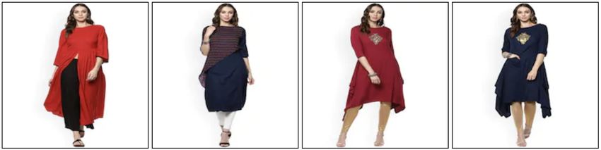
embeddings as a de facto standard, for all the methods.
                                                                               Effect of Batch Size and Momentum Encoding in SSL
                                                                            for our task: For studying the effect of batch size in SSL for
                                                                            our task, we introduce a third variant of SimSiam, i.e., Sim-
                                                                            Siam v2: This is essentially SimSiam v1 with a batch size of
                                                                            128. We then consider SimSiam v1, SimSiam v2 and BYOL,
                                                                            where the first makes use of a batch size of 12, while the others
                                                                            make use of batch sizes of 128. We observed that a larger batch
                                                                            size usually leads to a better performance. This is observed
                                                                            from Table 2, by the higher values of performance metrics
                  (a)                         (b)                           in the columns for SimSiam v2 and BYOL (vs SimSiam v1).
Figure 5: (a) Convergence behaviour of SimSiam v0: Validation               Additionally, we noted that the momentum encoder used in
of the fact that SimSiam actually converges (while avoiding model           BYOL causes a further boost in the performance, as observed
collapse) with an arbitrary data augmentation. (b) Convergence              in its superior performance as compared to SimSiam v2 that
behaviour of SimSiam v1: Considering standard augmentations with            has the same batch size. It should be noted that except for the
random crops leads to a better convergence.                                 momentum encoder, the rest of the architecture and augmenta-
                        SimSiam v0                SimSiam v1                tions used in BYOL are exactly the same as in SimSiam. We
    Dataset    Metric       (w/o     SimSiam v0       (w/o     SimSiam v1
                           norm)                     norm)                  observed that increasing the batch size in SimSiam does not
    Data 1     CGacc         0.5         0.5           1          0.67      drastically or consistently improve its performance, something
    Data 2     CGacc         0.5        0.67           0          0.25
    Data 3     CGacc          0          0.4           0          0.33      which its authors also noticed [Chen and He, 2021].
              Table 1: Effect of Embedding Normalization.                      Effect of Memory Queue in SSL for our task: We also
                                                                            inspect the effect of an extra memory module/queue being used
variants identification. For this purpose, we make use of a                 to facilitate the comparisons with a large number of negative
single Table 2, where we provide the comparison of various                  examples. In particular, we make use of the MOCOv2 method
SSL methods, including ours.                                                with the following settings: i) queue size of 5k, ii) temperature
    Convergence behavior with data augmentation for                         parameter of 0.05, iii) a MLP (512→4096→relu→123) added
our task: For illustrating how the convergence behavior                     after the avgpool layer of the ResNet34, iv) SGD for updating
of SSL methods changes with respect to a different data                     the query encoder, with learning rate of 0.001, momentum
augmentation, we pick the SimSiam SSL method for its                        of 0.9, weight decay of 1e−6 , and v) value of 0.999 for θ
simplicity and strong claims. We consider two variants of                   in the momentum update. It is observed from Table 2, by
SimSiam: i) SimSiam v0: A version of SimSiam, where                         the columns of MOCOv2 and BYOL, that the performance
we used the entire original image as the query, and a color                 of the former is superior. As BYOL does not use a memory
jittered image as the positive, and with a batch size of 12,                module, but MOCOv2 does, we conclude that using a separate
and ii) SimSiam v1: A version of SimSiam with standard                      memory module significantly boosts the performance of SSL
SSL [Chen et al., 2020] augmentations (ColorJitter,                         in our task. Motivated by our observations so far, we choose
RandomGrayscale,                RandomHorizontalFlip,                       to employ both momentum encoding and memory module in
GaussianBlur and RandomResizedCrop), and a                                  our proposed PBCNet method.
batch size of 12. For all cases, the following architec-
ture has been used for SimSiam: Encoder{ ResNet34                           4.2   Comparison of PBCNet against the
→ (avgpool) → ProjectorMLP(512→4096→123)                                          state-of-the-art
}→PredictorMLP(123→4096→123).                                               In Table 2, we provide the comparison of our proposed self-
    Figure 5a shows the convergence behaviour of SimSiam v0.                supervised method PBCNet against various self-supervised
It can be seen that SimSiam actually converges with an ar-                  state-of-the-art baselines and the supervised baseline across
bitrary data augmentation, while avoiding a model collapse                  all the datasets. It should be noted that in Table 2, any perfor-
even without making use of negative pairs. Figure 5b shows                  mance gains for a specific method is due to the intrinsic nature
the convergence behaviour of SimSiam v1. We observed that                   of the same, and not because of a particular hyperparameter
considering standard augmentations with random crops leads                  setting. This is because we report the best performance for
to a better convergence than that of SimSiam v0. Thus, for                  each method after adequate tuning of distance threshold (de-
all other self-supervised baselines, i.e., BYOL and MOCOv2                  tails in supplementary) and other parameters, and not just their
we make use of standard augmentations with random crops.                    default hyperparameters. Following are the configurations that
However, we later show that our proposed way of considering                 we have used in our PBCNet method: i) memory module size
multiple patches in PBCNet leads to a better performance.                   of 5k, ii) temperature parameter of 0.05, iii) the FC layer after
    Effect of l2 normalization for our task: Table 1 shows                  the avgpool layer of the ResNet34 was removed, iv) SGD for
the effect of performing l2 normalization on the embeddings                 updating the query encoder, with learning rate of 0.001, mo-
obtained using SimSiam. We found that without using any nor-                mentum of 0.9, weight decay of 1e−6 , and v) value of 0.999
malization, in some cases (eg, Data 2-3) there are no true color            for θ in the momentum update.
variant groups out of the detected clusters (i.e., zero precision),            We made use of a batch size of 32(= 128/4) as we
and hence the performance metrics become zero. Thus, for all                have to store tensors for each of the 4 slices simulta-
our later experiments, we make use of l2 normalization on the               neously for each mini-batch (we used a batch size of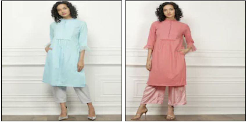
Supervised Self-Supervised
Dataset Metric Triplet Net SimSiam v0 SimSiam v1 SimSiam v2 BYOL MOCOv2 PBCNet (Ours)
Data 1 CGacc 0.67 0.5 0.67 1 0.5 1 1
Data 2 CGacc 1 0.67 0.25 1 0.75 0.8 0.75
Data 3 CGacc 0.75 0.4 0.33 0 0.5 0.5 0.6
CGacc 0.67 0.4 0.5 0.5 0.5 1 0.85
ARI 0.69 0.09 0.15 0.12 0.27 0.66 0.75
Data 4
FMS 0.71 0.15 0.22 0.20 0.30 0.71 0.76
CScore 0.700 0.110 0.182 0.152 0.281 0.680 0.756
CGacc 1 0 0.5 0.33 0.5 1 1
ARI 1 0 0.09 0.28 0.64 1 1
Data 5
FMS 1 0.22 0.30 0.45 0.71 1 1
CScore 1 0 0.135 0.341 0.674 1 1
CGacc 0.83 0.5 0.5 0.8 0.6 1 1
ARI 0.44 0.07 0.06 0.04 0.20 0.58 0.79
Data 6
FMS 0.49 0.12 0.17 0.13 0.24 0.64 0.80
CScore 0.466 0.089 0.090 0.063 0.214 0.610 0.796
Table 2: Comparison of our proposed method against the supervised and state-of-the-art self-supervised baselines, across all the datasets.
Dataset Data 4 Data 5 Data 6
Method Clustering ARI FMS ARI FMS ARI FMS
PBCNet Agglo 0.75 0.76 1.00 1.00 0.79 0.80
DBSCAN 0.66 0.71 1.00 1.00 0.66 0.71
Affinity 0.30 0.42 0.22 0.41 0.24 0.37
MOCOv2 Agglo 0.66 0.71 1.00 1.00 0.58 0.64
DBSCAN 0.66 0.71 1.00 1.00 0.37 0.40
Affinity 0.20 0.32 0.04 0.26 0.25 0.41
BYOL Agglo 0.27 0.30 0.64 0.71 0.20 0.24
DBSCAN 0.17 0.28 0.64 0.71 0.02 0.24
Affinity 0.03 0.14 0.28 0.45 0.01 0.11
Table 3: Effect of the clustering technique used.
Dataset Data 1 Data 2 Data 3 Data 4 Data 5 Data 6
Method CGacc CGacc CGacc CGacc ARI FMS CGacc ARI FMS CGacc ARI FMS
PBCNet-horiz 1 1 0.5 0.66 0.65 0.67 1 1 1 1 0.81 0.82
PBCNet-vert 1 0.6 0.6 1 0.88 0.89 1 1 1 0.83 0.48 0.50
b) MOCOv2
PBCNet 1 0.75 0.6 0.85 0.75 0.76 1 1 1 1 0.79 0.80
Table 4: Effect of Slicing on PBCNet
c) Supervised
information by virtue of the slicing (by borrowing information
from the other patches simultaneously), even with smaller
batches.
a) PBCNet
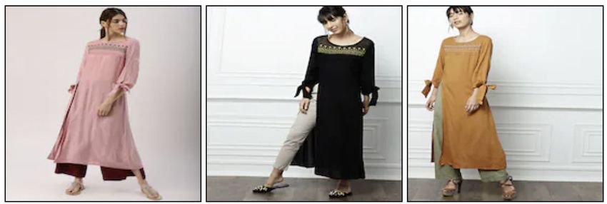
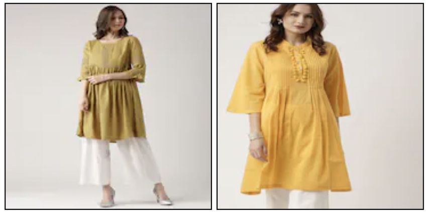
Figure 6: Qualitative comparison of color variants groups obtained We also noticed that the supervised baseline performs quite
using our PBCNet method (left column), MOCOv2 (middle column) good in our task, even without any data augmentation pipeline
and the supervised baseline (right column), on Data 4. as used in the SSL methods. However, by virtue of data
128 for the other methods). For data augmentation, we augmentations like color jitter and cropping, which are pretty
first apply a color distortion in the following order: i) relevant to the task of color variants identification, stronger
ColorJitter(0.8 * s, 0.8 * s, 0.8 * s, SSL methods like MOCOv2 and PBCNet are in fact capable
0.2 * s) with s=1, p=0.8, ii) RandomGrayscale with of surpassing the performance of the supervised baseline as
p=0.2, iii) GaussianBlur((3, 3), (1.0, 2.0)) well, in some cases. Having said that, if we do not have
with p=0.5. After the color distortion, we apply our slicing adequate labeled data in the first place, we cannot even use
technique. For the second image (positive/negative) we apply supervised learning. Hence, enabling data augmentations and
the same series of transformations. slicing strategy in the supervised model has not been focused,
From Table 2, it is clear that the SimSiam method despite its because the necessity of our approach comes from the issue
strong claims of not using any negative pairs, nor momentum of addressing the lack of labeled data, and not to improve the
encoder nor large batches, performs poorly as compared to performance of supervised learning (which any how is label
our supervised method (shown in bold blue color). The BYOL dependent).
method which also do not make use of negative pairs, performs Effect of Clustering: In Table 3, we report the perfor-
better than the SimSiam method in our use case, by virtue of mances obtained by varying the clustering algorithm to group
its momentum encoder. embeddings obtained by different SSL methods, on Data 4-6.
Among all compared SSL baselines, it is the MOCOv2 We picked the Agglomerative, DBSCAN and Affinity Prop-
method that performs the best. This is due to the reason of agation clustering techniques that do not require the number
the memory queue that facilitates the comparison with a large of clusters as input parameter (which is difficult to obtain in
number of negative examples. This shows that the impor- our use-case). In general, we observed that the Agglomera-
tance of considering negative pairs still holds true, especially tive clustering technique leads to a better performance in our
for challenging use-cases like the one considered in the pa- use-case. Also, for a fixed clustering approach, using embed-
per. However, our proposed self-supervised method PBCNet dings obtained by our PBCNet method usually leads to a better
clearly outperforms all the baselines. The fact that it outper- performance.
forms MOCOv2 can be attributed to the patch-based slicing Qualitative results: Sample qualitative comparisons of
used, which is the only different component in our method color variants groups obtained on Data 4 using our PBCNet
in comparison to MOCOv2 that uses random crop. Another method, MOCOv2 and the supervised baseline are provided
interesting thing that we observed is the fact that despite using in Figure 6. Each of the rows for a column corresponding to
much lesser batch size of 32, our method outperforms the a method represents a detected color variants cluster for the
baselines. In a way, we were able to extract and leverage more considered method. A row has been marked with a red box if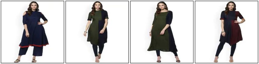
is how a human identifies color variants as well, by looking
MOCOv2 at the article along both horizontal and vertical directions, to
identify distinctive patterns. Even humans cannot identify an
Data 2
object if we restrict our vision to only a particular small crop.
PBCNet
Effect of the slicing: We also study 2 variants of our PBC-
Net method: i) PBCNet-horiz (computing an embedding only
by considering the top and bottom slices), and ii) PBCNet-vert
(computing an embedding using only the left and right slices).
MOCOv2 The results are shown in Table 4. In Data 4, PBCNet-vert
performs better than PBCNet-horiz, and in Data 6, PBCNet-
Data 3
horiz performs better than PBCNet-vert (significantly). The
PBCNet
performance of the two versions is also illustrated in Figure 8.
We observed that a single slicing do not work in all scenarios,
especially for apparels.
Figure 7: A few groups obtained on Data 2 & 3 using MOCOv2 have
false positives (shown in red box), while our PBCNet method does
Although the horizontal slicing is quite competitive, it may
not yield such groups. be beneficial to consider the vertical slices as well. This is
observed by the drop in performance of PBCNet-horiz in Data
3-4 (vs PBCNet). This is because some garments may con-
tain distinguishing patterns that may be better interpreted only
by viewing vertically, for example, printed texts (say, adidas
c) PBCNet-horiz success case on Data 6. The detected cluster is correct and
has a distinguishing pattern that is better captured with a horizontal slice.
written vertically), floral patterns etc. In such cases, simply
a) PBCNet-horiz failure case on Data 4: A row denotes
considering horizontal slices may actually split/ disrupt the
a cluster. The two detected clusters are incorrect. vertical information. It may also happen that mixing of slicing
introduces some form of redundancy, as observed by the oc-
casional drop in the performance of PBCNet when compared
to PBCNet-horiz (on Data 6) and PBCNet-vert (on Data 4).
d) PBCNet-vert failure case on Data 6. The detected cluster has a false
However, on average PBCNet leads to an overall consistent
positive. A vertical slice is not suitable in this case. and competitive performance, while avoiding drastically fluc-
tuating improvements or failures. We suggest considering
b) PBCNet-vert success case on Data 4: A row denotes
a cluster. The two detected clusters are correct. both the directions of slicing, so that they could collectively
Figure 8: Trade off between vertical and horizontal slicing. represent all necessary and distinguishing patterns, and if one
the entire cluster contains images that are not color variants slicing misses some important information, the other could
to each other. A single image is marked with a red box if compensate for it.
it is the only incorrect image, while rest of the images are
color variants. We observed that our method not only detects 5 Conclusions
clusters with higher precision (which MOCOv2 does as well), In this paper, we utilize deep visual Representation Learning to
but it also has a higher recall, which is comparable to the address the problem of identification of color variants (images
supervised method. We also make use of a blue box to show of objects exactly similar in design, but not color), particularly
a detected color group by our method which contains images for fashion products. A supervised triplet loss based deep
that are color variants, but are difficult to be identified at a first neural network model for visual Representation Learning has
glance. been proposed to identify the color variants. A systematic
Additionally, Figure 7 shows a few color groups identified in study of existing state-of-the-art self-supervised methods has
the datasets Data 2 & 3 using MOCOv2 and our PBCNet. We been done to solve the proposed problem, while alleviating
observed that MOCOv2 detected groups with false positives, the need for manual annotations. Also, a novel contrastive
while our PBCNet method did not. This could happen because loss based self-supervised representation learning method that
when a random crop is obtained by MOCOv2, it need not focuses on parts of an object has been proposed. This is
necessarily be from a distinctive region of an apparel that done to make the model better informed of the discriminative
helps to identify its color variant (eg, in Figure 7, the bent regions of an image, in order to identify color variants.
line like pattern separating the colored and black region of the
apparels of Data 2, and the diamond like shape in the apparels
of Data 3). We argue that a random crop might have arrived References
from such a distinctive region given that the size of the crop is [Cao et al., 2019] Xuefei Cao, Bor-Chun Chen, and Ser-Nam Lim.
made larger, etc. But that still leaves things to random chance. Unsupervised deep metric learning via auxiliary rotation loss.
On the other hand, our slicing technique being deterministic arXiv preprint arXiv:1911.07072, 2019.
in nature, guarantees that all the regions of an object would [Chen and He, 2021] Xinlei Chen and Kaiming He. Exploring sim-
be captured. We would also like to mention that our slicing ple siamese representation learning. Proc. of IEEE Conference on
approach is agnostic to the fashion apparel type, i.e, the same Computer Vision and Pattern Recognition (CVPR), 2021.
is easily applicable for any fashion article type (Tops, Shirts, [Chen et al., 2020] Ting Chen, Simon Kornblith, Mohammad
Shoes, Trousers, Track pants, Sweatshirts, etc). In fact, this Norouzi, and Geoffrey Hinton. A simple framework for con-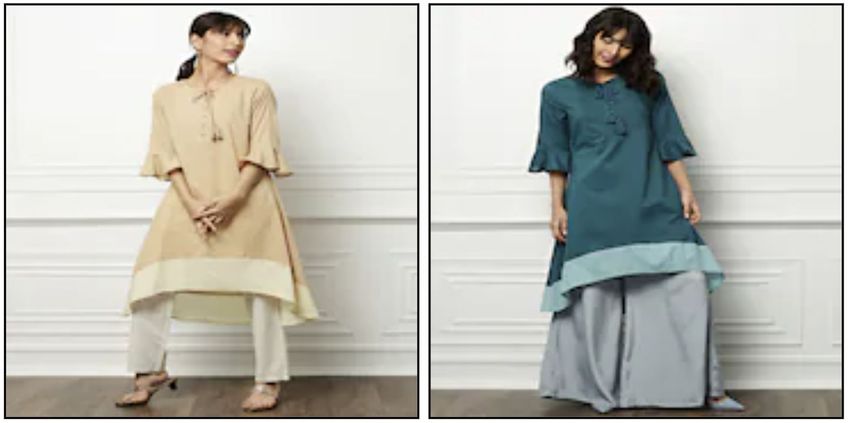
trastive learning of visual representations. In Proc. of Interna- [Veit et al., 2017] Andreas Veit, Serge Belongie, and Theofanis Kar-
tional Conference on Machine Learning (ICML), pages 1597– aletsos. Conditional similarity networks. In Proc. of IEEE Confer-
1607. PMLR, 2020. ence on Computer Vision and Pattern Recognition (CVPR), pages
830–838, 2017.
[Dutta et al., 2020a] Ujjal Kr Dutta, Mehrtash Harandi, and C Chan-
dra Sekhar. Unsupervised metric learning with synthetic examples. [Wang et al., 2018] Guanshuo Wang, Yufeng Yuan, Xiong Chen,
In Proc. of Association for the Advancement of Artificial Intelli- Jiwei Li, and Xi Zhou. Learning discriminative features with
gence (AAAI), 2020. multiple granularities for person re-identification. In Proc. of
ACM International Conference on Multimedia (ACMMM), pages
[Dutta et al., 2020b] Ujjal Kr Dutta, Mehrtash Harandi, and 274–282, 2018.
Chellu Chandra Sekhar. Unsupervised deep metric learning via
orthogonality based probabilistic loss. IEEE Transactions on
Artificial Intelligence (TAI), 1(1):74–84, 2020.
6 Supplementary: Additional Details and
[Grill et al., 2020] Jean-Bastien Grill, Florian Strub, Florent Altché,
Results (omitted from the main text due to
Corentin Tallec, Pierre H Richemond, Elena Buchatskaya, Carl space constraints)
Doersch, Bernardo Avila Pires, Zhaohan Daniel Guo, Mo- We evaluated the discussed methods on a large (orders of mag-
hammad Gheshlaghi Azar, et al. Bootstrap your own latent: nitudes of 105 ) internal collection of challenging real-world
A new approach to self-supervised learning. arXiv preprint industrial images on our Myntra platform (www.myntra.com)
arXiv:2006.07733, 2020.
that hosts various fashion products. In this section, we report
[Gu and Ko, 2020] Geonmo Gu and Byungsoo Ko. Symmetrical our results on a collection of roughly3 0.13 million Kurtas
synthesis for deep metric learning. In Proc. of Association for the images from our internal database. A disjoint set of 6k images
Advancement of Artificial Intelligence (AAAI), 2020. were manually annotated by our in-house team to provide class
[He et al., 2016] Kaiming He, Xiangyu Zhang, Shaoqing Ren, and labels indicating their color variants information. This labeled
Jian Sun. Deep residual learning for image recognition. In Proc. data was used to form triplets to train the supervised triplet
of IEEE Conference on Computer Vision and Pattern Recognition loss based color variants model. We also used the exact same
(CVPR), pages 770–778, 2016. set to train the self-supervised methods for a fair comparison.
[He et al., 2020] Kaiming He, Haoqi Fan, Yuxin Wu, Saining Xie,
For inferencing, we used the entire 0.13 million Kurtas im-
and Ross Girshick. Momentum contrast for unsupervised visual ages, which are present in the form of different dataset splits
representation learning. In Proc. of IEEE Conference on Computer (based on brand, gender, MRP). We refer to our 6 dataset splits
Vision and Pattern Recognition (CVPR), pages 9729–9738, 2020. as Data 1-6. Table 5 provides details of the datasets used to
compare the methods, along with their meta-data on our plat-
[Jagadeesh et al., 2014] Vignesh Jagadeesh, Robinson Piramuthu, form. It should be noted that the datasets Data 1-3 do not have
Anurag Bhardwaj, Wei Di, and Neel Sundaresan. Large scale manual annotations available for them, whereas the remaining
visual recommendations from street fashion images. In Proc. of
ACM Special Interest Group on Knowledge Discovery and Data
three have been annotated by the taggers.
Mining (SIGKDD), pages 1925–1934, 2014. Ground Truth
Dataset Article Type Gender Brand MRP
Available
[Jing and Tian, 2020] Longlong Jing and Yingli Tian. Self- Data 1 Kurtas Women STREET 9 1899 No
supervised visual feature learning with deep neural networks: Data 2
Data 3
Kurtas
Kurtas
Women
Women
STREET 9
STREET 9
1399
1499
No
No
A survey. IEEE Transactions on Pattern Analysis and Machine Data 4 Kurtas Women all about you 1699 Yes
Intelligence (TPAMI), 2020. Data 5 Kurtas Women all about you 2499 Yes
Data 6 Kurtas Women all about you 2199 Yes
[Levi et al., 2020] Elad Levi, Tete Xiao, Xiaolong Wang, and Trevor Table 5: Details of datasets used to compare the methods.
Darrell. Reducing class collapse in metric learning with easy Dataset Config Sup S0 S1 S2 B M PB
t 1 0.07 0.3 0.3 0.5 0.7 0.8
positive sampling. arXiv preprint arXiv:2006.05162, 2020. Data 1 nCG 2 1 2 1 1 2 2
nDG 3 2 3 1 2 2 2
[Li et al., 2020] Yang Li, Shichao Kan, and Zhihai He. Unsuper- t 0.87 0.07 0.15 0.2 0.5 0.8 0.8
Data 2 nCG 4 2 1 2 3 4 3
vised deep metric learning with transformed attention consistency nDG 4 3 4 2 4 5 4
t 0.87 0.2 0.24 0.3 0.5 0.8 0.8
and contrastive clustering loss. In Proc. of European Conference Data 3 nCG 3 2 2 0 1 3 3
nDG 4 5 6 5 to 7 2 6 5
on Computer Vision (ECCV), 2020. t 0.8 0.1 0.1 0.5 0.5 0.6 0.8
Data 4 nCG 4 2 1 3 3 3 6
[Redmon and Farhadi, 2017] Joseph Redmon and Ali Farhadi. nDG 6 5 2 6 6 3 7
t 0.9 0.3 0.6 0.6 0.7 0.7 0.8
Yolo9000: better, faster, stronger. In Proc. of IEEE Conference on Data 5 nCG 1 0 1 1 1 1 1
nDG 1 1 2 3 2 1 1
Computer Vision and Pattern Recognition (CVPR), pages 7263– t 0.95 0.07 0.8 0.8 0.6 0.8 0.9
7271, 2017. Data 6 nCG
nDG
5
6
2
4
2
4
4
5
3
5
6
6
7
7
[Schroff et al., 2015] Florian Schroff, Dmitry Kalenichenko, and Table 6: Distance thresholds in Agglomerative clustering used to
James Philbin. Facenet: A unified embedding for face recognition produce the best results (for each method) across all the datasets,
and clustering. In Proc. of IEEE Conference on Computer Vision along with the number of detected and correct color groups.
and Pattern Recognition (CVPR), pages 815–823, 2015. NOTE that we have used the following notations: Config: Con-
figuration, t:threshold, nCG:n correct gps, nDG:n detected gps,
[Sun et al., 2020] Yifan Sun, Changmao Cheng, Yuhan Zhang, Chi Sup:Supervised, S0:SimSiam v0, S1:SimSiam v1, S2:SimSiam v2,
Zhang, Liang Zheng, Zhongdao Wang, and Yichen Wei. Circle B:BYOL, M:MOCOv2, and PB:PBCNet.
loss: A unified perspective of pair similarity optimization. In Proc.
3
of IEEE Conference on Computer Vision and Pattern Recognition Company compliance policies prohibit open-sourcing/ revealing
(CVPR), pages 6398–6407, 2020. exact dataset specifics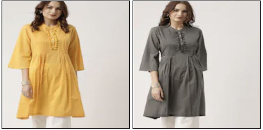
Method SimSiam v0 Method SimSiam v1 Method SimSiam v2
Dataset dist threshold CGacc ARI FMS Dataset dist threshold CGacc ARI FMS Dataset dist threshold CGacc ARI FMS
0.07 0.5 0.2 1 0.3 1
Data 1 0.1 0.33 0.3 0.67 Data 1 0.5 0.5
Data 1
0.2 0.33 0.4 0.5 0.6 0.5
0.07 0.67 0.5 0.67 0.2 1
Data 2 0.1 0.4 0.15 0.25 0.3 0.4
Data 2
0.2 0.25 Data 2 0.2 0.2 0.4 0.5
0.07 0 0.3 0.2 0.5 0.5
Data 3 0.1 0 0.1 0 0.2 0
0.2 0.4 0.2 0.2 Data 3 0.3 0
Data 4 0.1 0.4 0.09 0.15 0.23 to 0.25 0.33 0.5 0
Data 3
Data 5 0.3 0 0.00 0.22 0.3 0.33 0.3 0.33 0.14 0.18
Data 4
0.07 0.5 0.07 0.12 0.4 0.16 0.5 0.5 0.12 0.20
Data 6
0.1 0.4 0.01 0.08 0.6 0 0.6 0.33 0.28 0.45
Data 5
0.1 0.5 0.15 0.22 1.1 0.5 0.09 0.30
Data 4
0.2 0.14 0.03 0.08 0.6 0.33 0.02 0.09
Data 5 0.6 0.5 0.09 0.30 Data 6 0.8 0.8 0.04 0.13
0.4 0.4 0.05 0.14 0.9 0.75 0.01 0.11
Data 6
0.8 0.5 0.06 0.17
Method BYOL Method MOCOv2 Method PBCNet
Dataset dist threshold CGacc ARI FMS Dataset dist threshold CGacc ARI FMS Dataset dist threshold CGacc ARI FMS
0.5 0.5 0.6 1 0.6 1
Data 1 0.7 0.5 0.7 1 0.7 1
Data 1
1.1 0.33 0.8 0.67 Data 1 0.8 1
0.5 0.75 0.9 0.5 0.9 0.67
Data 2 0.7 0.6 0.6 0 1 0.5
0.9 0.6 0.7 1 0.6 1
Data 2
0.5 0.5 0.8 0.8 0.8 0.75
Data 2
0.55 0.33 0.9 0.67 0.9 0.75
Data 3 0.6 0.25 0.6 0.5 1 0.67
0.7 0.33 0.7 0.5 0.6 0.5
Data 3
0.9 0.28 0.8 0.5 0.7 0.33
0.3 0.5 0.15 0.22 0.9 0.42 Data 3 0.8 0.6
Data 4 0.45 0.33 0.22 0.26 0.5 1 0.17 0.32 0.9 0.42
0.5 0.5 0.27 0.30 0.6 1 0.66 0.71 1 0.42
0.7 0.5 0.64 0.71 Data 4 0.7 0.57 0.49 0.53 0.5 1 0.32 0.45
Data 5
0.8 0.33 0.46 0.58 0.8 0.67 0.37 0.47 0.6 1 0.45 0.55
0.55 0.67 0.12 0.16 0.9 0.6 0.29 0.42 Data 4 0.7 1 0.74 0.77
Data 6
0.6 0.6 0.20 0.24 0.7 1 1.00 1.00 0.8 0.85 0.75 0.76
Data 5 0.8 0.5 0.64 0.71 0.9 0.85 0.65 0.68
0.9 0.33 0.28 0.45 0.6 1 1.00 1.00
0.6 1 0.39 0.50 0.7 1 1.00 1.00
Data 5
0.7 0.67 0.34 0.37 0.8 1 1.00 1.00
0.8 1 0.58 0.64 0.9 0.5 0.64 0.71
0.9 0.85 0.56 0.65 0.6 1 0.39 0.50
Data 6
0.7 1 0.66 0.71
Data 6 0.8 1 0.70 0.72
0.9 1 0.79 0.80
1 1 0.47 0.53
Table 7: Varying values of performance metrics against distance thresholds. For a method, only those thresholds are reported against a dataset,
using which Agglomerative Clustering produces non-zero performance metrics, thus indicating a meaningful clustering.
Performance metrics used: To evaluate the methods, we ber of pairs that belong to the same clusters in both the
made use of the following performance metrics (CGacc and ground truth, as well as the predicted cluster labels, F P
CScore are defined by us for our use-case): is the number of pairs that belong to the same clusters
in the ground truth, but not in the predicted cluster la-
1. Color Group Accuracy (CGacc): It refers to the ratio of bels, and F N is the number of pairs that belong in the
the number of correct color groups to that of the number same clusters in the predicted cluster labels, but not in
of detected color groups. Here, detected color groups the ground truth.
are the clusters identified by the clustering algorithm that 4. Clustering Score (CScore): It is computed as:
have a size of at least two. A correct color group is a CScore = 2.ARI.F MS
ARI+F M S .
cluster among the detected color groups, which contains It should be noted that while we use CGacc to compare the
at least half of its examples which are actually color methods for all the datasets (Data 1-6), the remaining metrics
variants to each other (while implementing we take a are reported only for the datasets Data 4-6, where we have
floor function). It should be noted that this performance the ground-truth labels. Also, all the performance metrics take
metric has a direct business relevance due to the fact that values in the range [0, 1], where a higher value indicates a
it reflects the precision. Also, it is computed by our in- better performance.
house catalog team by performing manual Quality Check Also, for each method, the distance threshold used to obtain
(QC). the results, and the corresponding number of detected as well
2. Adjusted Random Index (ARI): Let s (and d, respec- as the number of correct groups obtained, are reported in Table
tively) be the number of pairs of elements that are in 6. From Table 6, we observed that our method is capable of
the same (and different, respectively) set in the ground detecting more number of color groups with a usually higher
truth class assignment, and in the same (and different, precision, when compared to its competitors.
respectively) set in the clustering. Then, the (unadjusted) In Table 7, we report the performance of all the compared
Random Index is computed as: RI = Ns+d C2
, where N self-supervised methods (including ours) on all the datasets,
is the number of elements clustered. The Adjusted RI with respect to the different metrics against varying values of
RI−E[RI]
(ARI) is then computed as: ARI = max(RI)−E[RI] . ARI the distance threshold used in the Agglomerative clustering.
ensures that a random label assignment will get a value
close to zero (which RI does not).
3. Fowlkes-Mallows Score (FMS): It is computed as:
TP
FMS = √ , where T P is the num-
(T P +F P )(T P +F N )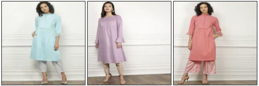
You can also read