Graphical Dispersion Plot Editor (DPE) for Seismic-Site Characterization by Using Multiple Surface-Wave Methods - MULTIPLE METHODS ACTIVE
←
→
Page content transcription
If your browser does not render page correctly, please read the page content below
Graphical Dispersion Plot Editor (DPE) for Seismic-Site
Characterization by Using Multiple Surface-Wave Methods

                                  MULT IPL E ME T HODS

                       ACTIVE                      PASSIVE

Open-File Report 2020–1065

U.S. Department of the Interior
U.S. Geological Survey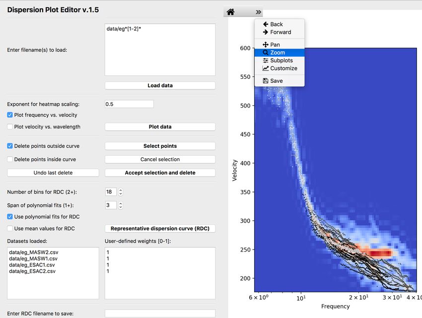
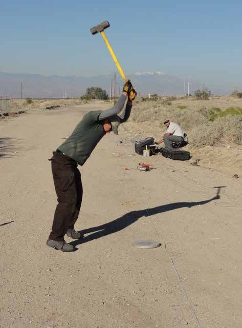
Cover. Left, Photograph showing Antony Martin (midground) and Will Dalrymple (foreground) of
GEOVision, collecting active-source MASW data with a linear array of seismometers. Right, Photograph
showing Antony Martin monitoring equipment during ambient-noise (passive) data collection at the same
site. Photographs by Alan Yong, U.S. Geological Survey.
Graphical Dispersion Plot Editor (DPE) for Seismic-Site
Characterization by Using Multiple Surface-Wave Methods

By Devin McPhillips, Alan K. Yong, Antony Martin, and William J. Stephenson

Open-File Report 2020–1065

U.S. Department of the Interior
U.S. Geological Survey
U.S. Department of the Interior DAVID BERNHARDT, Secretary U.S. Geological Survey James F. Reilly II, Director U.S. Geological Survey, Reston, Virginia: 2020 For more information on the USGS—the Federal source for science about the Earth, its natural and living resources, natural hazards, and the environment—visit https://www.usgs.gov or call 1–888–ASK–USGS. For an overview of USGS information products, including maps, imagery, and publications, visit https://store.usgs.gov/. Any use of trade, firm, or product names is for descriptive purposes only and does not imply endorsement by the U.S. Government. Although this information product, for the most part, is in the public domain, it also may contain copyrighted materials as noted in the text. Permission to reproduce copyrighted items must be secured from the copyright owner. Suggested citation: McPhillips, D.F., Yong, A.K., Martin, A., and Stephenson, W.J., 2020, Graphical Dispersion Plot Editor (DPE) for seismic-site characterization by using multiple surface-wave methods: U.S. Geological Survey Open-File Report 2020–1065, 8 p., https://doi.org/10.3133/ofr20201065. ISSN 2331-1258 (online)
iii

Contents
Introduction����������������������������������������������������������������������������������������������������������������������������������������������������1
Method for Calculating the Representative Dispersion Curve��������������������������������������������������������������2
Weighting the Data����������������������������������������������������������������������������������������������������������������������������������������2
System Requirements and Installation Instructions��������������������������������������������������������������������������������2
Input and Output Conventions���������������������������������������������������������������������������������������������������������������������3
Quick-Start Guide������������������������������������������������������������������������������������������������������������������������������������������3
Workflow Example�����������������������������������������������������������������������������������������������������������������������������������������4
Troubleshooting����������������������������������������������������������������������������������������������������������������������������������������������7
References Cited�������������������������������������������������������������������������������������������������������������������������������������������8

Figures
         1.     Screenshot showing example of the Dispersion Plot Editor (DPE) version 1.5
                graphical interface after loading and plotting data����������������������������������������������������������������3
         2.     Screenshot showing example of data selection and deletion����������������������������������������������5
         3.     Screenshot showing example following the first deletion of spurious data����������������������6
         4.     Screenshot showing example of a representative dispersion curve (RDC) plot���������������6
         5.     Screenshot showing example of saving data��������������������������������������������������������������������������7

Abbreviations
DPE                Dispersion Plot Editor
ESAC               extended spatial autocorrelation
MASW               multichannel analysis of surface waves
RDC                representative dispersion curve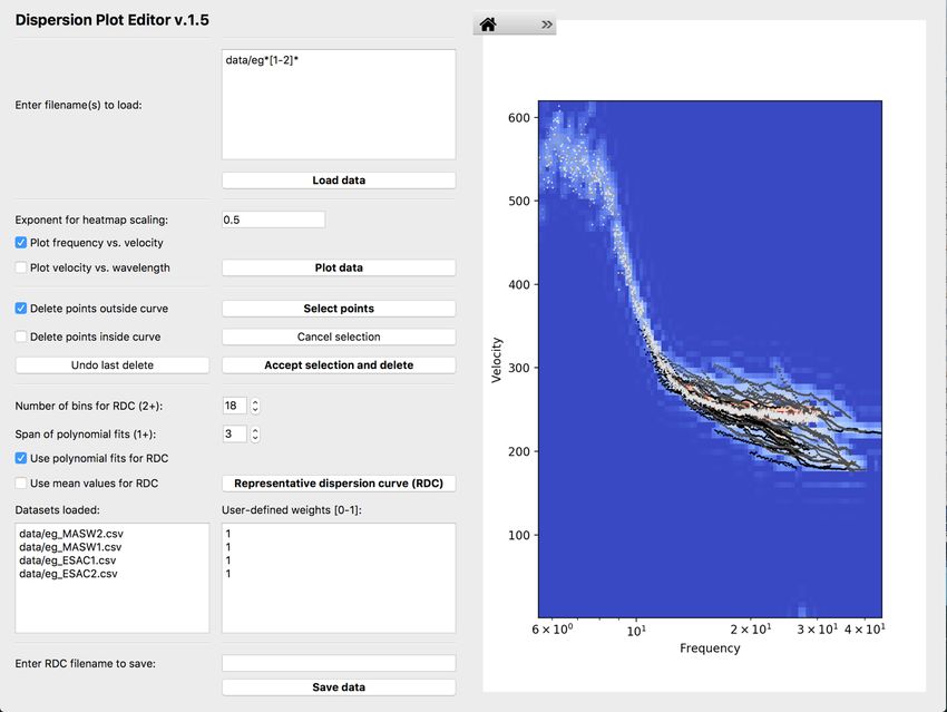
Graphical Dispersion Plot Editor (DPE) for Seismic-Site
Characterization by Using Multiple Surface-Wave Methods

By Devin McPhillips,1 Alan K. Yong,1 Antony Martin,2 and William J. Stephenson1

Introduction                                                              Spurious data may be identified and mitigated by com-
                                                                    bining dispersion data derived from multiple methods at a
      To understand the behavior of potentially damaging            single site (Martin and others, 2017; Yong and others, 2019).
ground motions during earthquakes, seismic-site effects             For example, passive source methods usually resolve lower
are routinely characterized by using the dispersion of sur-         frequencies, and consequently deeper structure, than active
face waves. Many methods exist to measure dispersion (for           source methods (Stephenson and others, 2005; Yong and oth-
example, Stokoe and others, 1988; Foti, 1999; Park and others,      ers, 2013; Martin and others, 2017). Combining dispersion
1998, 1999; Okada, 2003; Louie, 2001; Martin and others,            data from both active and passive methods produces the best
2014). These methods have various advantages and disadvan-          possible resolution over the largest possible frequency domain.
tages, but they all yield dispersion data that must be inverted     In addition, the overlapping region of intermediate frequen-
for shear-wave velocity. This report presents a graphical tool      cies provides an opportunity to verify the interpretation of
for efficiently removing spurious data as well as combining         fundamental-mode data (Martin and others, 2017; Yong and
data from multiple methods prior to inversion (Yong and oth-        others, 2019).
ers, 2013; Martin and others 2017; Yong and others, 2019).                An important limitation of the multiple-method approach
      The Dispersion Plot Editor (DPE) program presented            is that it yields datasets with too many points for easy inver-
here (version 1.5) is coded in Python 3, which is open source       sion. The forward-model calculation of dispersion data from a
and platform independent. DPE accepts input dispersion data         layered velocity model is computationally intensive (Haskell,
as one or more delimited text files. The program plots the data     1953). As a result, the time required for global inversions of
in useful forms, including both scattered points and an inter-      large numbers of points is commonly prohibitive. Regularized
polated heat map. The user selects points to delete by drawing      linear inversions provide a faster alternative but may not
arbitrary shapes with the mouse cursor. After the spurious data     yield accurate results, especially when the velocity structure
are removed, the user may represent the acceptable data with a      is complex. To circumvent this limitation, dispersion data are
dispersion curve (Yong and others, 2013). The acceptable data       commonly summarized and reduced by using a combination
and the representative dispersion curve are output as separate      of manual editing and polynomial fitting. This approach yields
comma-delimited text files. Images of the plotted data and the      a representative dataset composed of the minimum number
representative dispersion curve may also be saved.                  of points that are amenable to rapid inversion. Furthermore,
      There are several potential sources of spurious dispersion    experience has shown this approach to yield accurate results
data. For example, the local site conditions may not conform        (Martin and others, 2017; Yong and others, 2019).
to the routine assumption of a flat, layered, one-dimensional             We anticipate that the DPE will be easily incorporated
half-space. In addition, different methods of measuring disper-     into many different site- characterization workflows because
sion data are sensitive in different frequency bands. The dis-      of its graphical implementation on an open-source plat-
persion signal may be contaminated by noise, causing error in       form. The Python language, in particular, is widely used in
data selection. In some instances, it may be especially difficult   geophysical-data processing (Beyreuther and others, 2010;
to discriminate the fundamental mode from higher modes, but         Megies and others, 2011; Krischer and others, 2015). We also
typically only the fundamental mode is used in velocity inver-      hope that the availability of this tool will speed the adoption
sions (Tokimatsu and others, 1992).                                 of multiple-method site characterization as a standard practice,
                                                                    yielding more accurate and reliable results (Yong and COS-
 1U.S.   Geological Survey
                                                                    MOS Guidelines Facilitation Committee, 2016; 2017; 2018;
                                                                    Yong and others, 2018).
 2Geovisions
2 Graphical Dispersion Plot Editor (DPE) for Seismic-Site Characterization by Using Multiple Surface-Wave Methods
Method for Calculating the E = ∑ j Wj 2 |y j − p(x j)| 2,
(1)
Representative Dispersion Curve where
yj is an observation,
The most important output of the DPE program is the p(xj) is a prediction at the frequency xj, and
representative dispersion curve (RDC; Yong and others, 2013; j is the index of a point within the domain of
Martin and others, 2017; Yong and others, 2019. The RDC this polynomial fit.
(1) combines dispersion data produced by multiple methods
The fit domain consists of a log-width bin and adjacent bins
and (2) reduces the total number of points in the dataset prior
as defined by the user. Points on the weighted-mean RDC are
to inversion. Inversion of the RDC should yield a robust
calculated by using a similar weighting term
shear-wave velocity model with minimal computational
time. Both of the two methods for calculating the RDC are _
y = (∑ Wk ) −1(∑ Wk y k), (2)
implemented in the DPE program, and both methods use a
weighting scheme described in the subsequent section.
Joh (1996) introduced a piecewise polynomial fit as where k is the index of a point within the current bin, and
a means of reducing the number of points in a dispersion the compound weight, W, at any point (j or k) is defined as
dataset prior to inversion. An adapted version of this method the product
was implemented here. By default, the data domain is in
units of frequency, but the user may alternatively choose to W = ab,
(3)
work in velocity-wavelength space. First, the domain of the
data is divided into a user-defined number of log-width bins. where a and b vary according to the input datasets.The first
Logarithmic bins are used because high frequencies typically component weight, a, is applied automatically to ensure that
yield much more data than low frequencies, especially for all input datasets have equal influence on the result, even if
active-source measurements, so log-width bins tend to distribute one dataset locally consists of many more points than another
data more evenly. The data are then fit to weighted second-order dataset. The value of a is identical for all points in the fit
polynomials with one polynomial associated with each bin. domain that are derived from the same input dataset and is
To achieve a smooth curve, however, each polynomial is fit calculated as the inverse of the total number of points in the
not only to the data in a single bin, but simultaneously to the fit domain in each dataset. The second weight, b, is defined by
data in adjacent bins. The user controls the smoothness of the the user in the interval from zero to one for each input dataset.
RDC by adjusting the number of adjacent bins included in Although b is set to 1 by default, it is sometimes useful to
the polynomial fits. The RDC is calculated by evaluating the manually adjust the weighting if the user has a reason to favor
appropriate polynomial at the midpoint of each bin except at the one dataset over another. Data collected on a two-dimensional
boundaries of the domain, where the polynomials are evaluated array, for example, might be given more weight than data from
near the edge of the bins to preserve the original domain size one-dimensional array.
in the RDC. The standard deviation of the data in each bin is
reported as a measure of the local precision of the RDC.
As an alternative to the piecewise polynomial method, the System Requirements and Installation
user may calculate the RDC by using weighted-mean values.
In this approach, the data are also binned logarithmically. Instructions
The weighted mean of the data in each bin is calculated and
reported at the midpoint of the bin; these data form the RDC. DPE was written and tested in the Anaconda distribution
Unlike the polynomial method, no additional smoothing is of Python 3; any computer system capable of running this
imposed. The standard deviation of the data in each bin is also distribution should also run DPE. Acceptable operating
reported as a measure of the local precision of the RDC. systems include Windows 7, macOS 10.10+, and many Linux
If neither the piecewise polynomial nor the weighted- distributions. DPE should also run in other distributions of
mean methods are acceptable, the user may calculate the RDC Python 3, although it has been minimally tested. The essential
by using an alternative method outside the DPE program. DPE libraries are PyQt 5, NumPy, SciPy, MatPlotLib, and Pandas.
outputs the complete edited datasets as delimited text files for In particular, PyQt 4 is not acceptable. A disadvantage
this purpose. of the Python language is that it is not fully backwards
compatible. The Anaconda Distribution is freely available at
https://www.anaconda.com.
Weighting the Data Installation of DPE simply requires copying the source
files to a folder in Python’s path; it is recommended to
The DPE employs a compound weighting scheme. dedicate a folder to DPE alone. There are four source files:
The polynomial-fit routine searches for the parameters that dpeExe.py, mplwidget.py, dpeUi_v1p5.py, and dpeAppFmwk_
minimize the sum of the weighted squared errors, E: v1p5.py. Because Python requires no explicit compiling byQuick-Start Guide 3
the user, these files are ready to use and also readable by the pattern-matching tools such as wildcards from the glob
user. To run DPE, call dpeExe.py from the command line. For module (https://docs.python.org/3/library/glob.html) to load
example: multiple files simultaneously. This method may be useful
if the user wishes to edit many dispersion data files with
:DPE dmcphillips$ python dpeExe.py systematically organized file names.
Output files are written as comma-separated values.
Input and Output Conventions By default, DPE writes N output files corresponding to the
number of input datasets when users save their work. The
Acceptable input files include any delimited text file, output files include “_trim” in the file names. Users may also
but they must have at least two columns and a header row specify a filename to use for additional output files containing
with column labels. Only “Velocity,” “Frequency,” and the RDC. The RDC file has four columns listing data for each
“Wavelength” are accepted as labels (DPE ignores columns bin: velocity, frequency, wavelength, and standard deviation.
beyond the third one), but the order of the columns and the The fourth column is a measure of the data scatter around the
delimiter do not matter. For example: RDC. Because DPE ignores the fourth column, the RDC file
may be subsequently loaded for additional editing.
Velocity Frequency Wavelength
560 5.76 97.1
552 5.80 95.2
... ... ... Quick-Start Guide
The user has considerable flexibility for loading input The following steps describe the use of DPE (fig. 1). A
files in DPE. For example, the user may enter a list of more detailed example is presented in the next section. First,
N individual file names. Alternatively, the user may use install and launch DPE from the command line.
Figure 1. Screenshot showing example of the Dispersion Plot Editor (DPE) version 1.5 graphical interface after loading
and plotting data. Input filename includes wildcards and the path name for the subdirectory containing the data files.
MASW data are plotted as dark gray points in the lower half of the plot; ESAC data are plotted as very light gray points.
To provide a constant frame of reference, the heatmap itself, which shows the densities of all points and is shaded, is not
updated as data are edited.4 Graphical Dispersion Plot Editor (DPE) for Seismic-Site Characterization by Using Multiple Surface-Wave Methods
1. Load data. Type filenames into the text box, one per
line, taking care to include any subdirectories (for
Workflow Example
example, data/file1.csv; data/file*.csv). Clicking the The capabilities of DPE are presented here with a detailed
“Load data” button more than once will overwrite workflow for combining active and passive data, trimming
previously loaded data with new data. spurious points, calculating a RDC, and saving the results in
2. Customize plotting options. Choose an exponent for an output file. This example is directed at the novice Python
the heat-map color scaling; values between 0.1 and user and formatted for macOS 10.10+. Although DPE may be
0.9 commonly reveal multiple data modes best. Use called from an interactive environment such as Spyder, it is
the check boxes to indicate whether to plot frequency usually more efficient to call DPE directly from the command
versus velocity (the default choice) or velocity versus line of a terminal application. To start, navigate to the DPE
wavelength. directory, and list its contents in a terminal application:
3. Plot data. The “Plot data” button plots currently loaded :~ dmcphillips$ cd Documents/PYTHON/DPE
datasets. Each dataset has a unique grayscale value. :DPE dmcphillips$ ls
Click again to change plotting options or clear an unde- dpeAppFmwk_v1p4.py
sirable RDC. dpeExe.py
dpeUi_v1p4.py
4. Select valid data. Use the checkboxes to indicate data
whether to select and delete points inside or outside a mplwidget.py
selection curve. Click “Select points” to activate the
selector tool. Draw a curve on the plot while holding The directory “data” contains five text files, data from active-
down the left mouse button. Click “Cancel selection” source Multi-channel Analysis of Surface Waves (MASW)
to start the process anew. Click “Accept selection and (Foti, 1999; Park and others, 1999) and passive-source
delete” to delete the selected data and plot the remain- Extended Spatial Auto-Correlation (ESAC) (Okada, 2003)
ing data again (note that the heat map does not change). measurements, respectively:
Click “Undo last delete” to revert. This process can be :DPE dmcphillips$ ls data
repeated as many times as necessary, alternating between eg_ESAC1.csv
deleting points inside and outside the selection curve. eg_ESAC2.csv
Consider saving the trimmed data now rather than later eg_MASW1.csv
in the process. eg_MASW2.csv
5. Define RDC methodology. Use the checkboxes to eg_MASW3.csv
indicate whether to use the polynomial or mean-value If all the files are present, call DPE:
method for calculating the RDC. If desired, adjust the :DPE dmcphillips$ python dpeExe.py
user-defined weights in the text box. RDCs are usu-
ally best defined by the use of 12–24 bins. For piece- This action should launch the graphical interface in a new
wise fits, polynomials should usually span fewer than window. For this example, consider the file eg_MASW3.csv to
about 5 bins. be part of a different site-characterization project. Load only
the four relevant datasets all at once by using wildcards (*)
6. Calculate the RDC. Click “Representative dispersion and brackets ([]). In the uppermost box, type:
curve (RDC)” to calculate and plot the RDC by using the
data/eg*[1-2]*
current options and data. Consider changing the method
and clicking again to view alternatives. Click “Plot data” and click the “Load data” button. This command creates
to clear the RDC plots. four datasets in DPE: two consisting of passive-source data
(ESAC) and another two consisting of active-source data
7. Save data. To save the RDC and trimmed data, type one (MASW). It also populates the “Datasets loaded” and
filename for the RDC in the text box and click “Save “User-defined weights” boxes. Note that the use of wildcards
data.” To save only the trimmed data, simply click “Save (*) and brackets ([]) is not required; entering all four complete
Data” at any time. Clicking more than once will cause filenames, or any combination of complete filenames,
the program to overwrite existing files. wildcards (*), and brackets ([]) would also work. See the
documentation for the glob module for additional information
8. Save plots. Use the “Save” option in the toolbar located
(https://docs.python.org/3/library/glob.html). To plot the
above the plot to save an image of the plot itself.
datasets in frequency space, simply click “Plot data” (fig. 1).
When one project is complete, close DPE and launch a fresh Otherwise, check the “Plot velocity vs. wavelength” box
window before loading new datasets. before clicking “Plot data.”Workflow Example 5
Each dataset is plotted as points with the same grayscale by checking the “Delete points outside curve” box. To zoom
value. The heatmap plotted behind the points is calculated into a small area, use the Zoom tool in the menu on the top
jointly from all of the datasets and is useful as a visual aid left corner of the heatmap (fig. 3). Users can select and delete
for interpreting different modes in the dispersion data. The points in as many iterations as necessary.
color scale can be adjusted by changing the exponent on the After the spurious data have been removed, calculate
power-law color normalization. This exponent is commonly the RDC from the acceptable data. First, enter the number
called the gamma value, and a value of 1 yields a linear color of bins by using the spinner box (a good starting point is
scale. Smaller values are useful for highlighting sparse data. 12–24). Second, choose the span of the polynomial fits in
Next, select and delete spurious data. Click on the the terms of a specified number of adjacent bins. Third, select
“Select points” button. This enables the cursor to draw on the the user-defined weights for each dataset by typing a number
plot while the left mouse button is depressed. Draw a curve between 0 and 1 in the “User-defined weights” box which is
around the high-quality data (fig. 2); there is no need to close adjacent to the list of the loaded datasets. In this example, the
the curve. In this example, higher modes are trimmed from passive and active datasets are given equal weight. Finally,
high-frequency data, and noise is trimmed from low-frequency click “Representative dispersion curve (RDC)” (fig. 4). If the
data. If the selection looks unsatisfactory, click on the RDC is not ideal, click “Plot data” to replot the edited data
“Cancel selection” button. Otherwise, click on the “Accept without the RDC, and try again by using different parameters.
selection and delete” button. The plot is redrawn without the When the RDC is satisfactory, save the data. To save only
spurious data. Note that the heatmap remains unchanged. It the edited datasets, simply click “Save data.” This command
is also possible to specifically delete small groups of points saves the edited datasets by appending “_trim” to the filename.
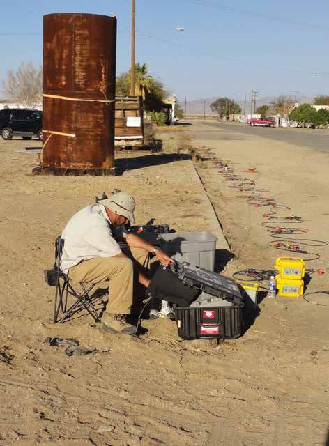
Figure 2. Screenshot showing example of data selection and deletion. Draw a curve to select data after clicking “Select
points.” In this case, the data outside the shape, which are primarily higher modes in the MASW data, will be deleted.6 Graphical Dispersion Plot Editor (DPE) for Seismic-Site Characterization by Using Multiple Surface-Wave Methods
Figure 3. Screenshot
showing example
following the first
deletion of spurious data.
The user may focus on
details of the plot by
using the zoom tool and
delete data by using
as many iterations as
necessary.
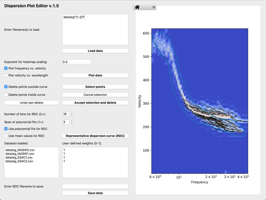
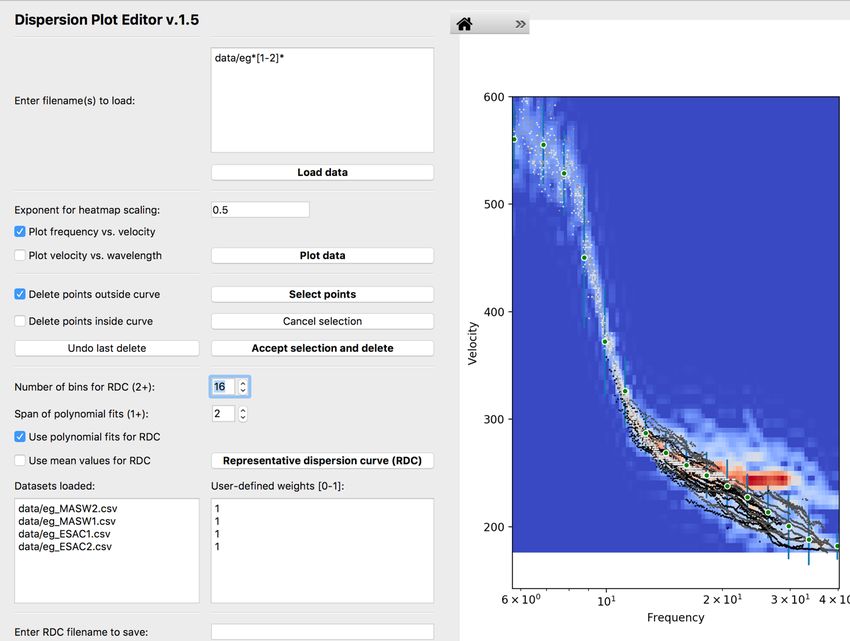
Figure 4. Screenshot
showing example
of a representative
dispersion curve (RDC)
plot. This example
uses 16 log-width bins
and fits a polynomial
through data in one
adjacent bin on each
side of each bin. Blue
bars represent the
range of the data
in each bin at two
standard deviations.
All of the user-defined
weights are equal to
the default value of 1.Troubleshooting 7
To save the RDC as well, enter one filename, including any
necessary directories, in the lower box, and click “Save data”
Troubleshooting
(fig. 5). Check that the save was successful. For simplicity, DPE employs minimal error checking
:DPE dmcphillips$ ls data beyond the native libraries. If the program is not behaving
eg_ESAC1.csv as expected, check the terminal window for error messages.
eg_ESAC2.csv For novice users, perhaps the most common errors result
eg_MASW1.csv from mistakes in the path and filenames. Recall that
eg_MASW2.csv filenames entered in DPE must include the prefix “data/”
eg_MASW3.csv if a subdirectory of datafiles is in use. Microsoft Excel is
eg_ESAC1_trim.csv sometimes useful for constructing input files by using “Save
eg_ESAC2_trim.csv as” and selecting the “.csv” extension.
eg_MASW1_trim.csv The DPE codes are available by request for no cost.
eg_MASW2_trim.csv Please report bugs to dmcphillips@usgs.gov.
testOutRDC.txt
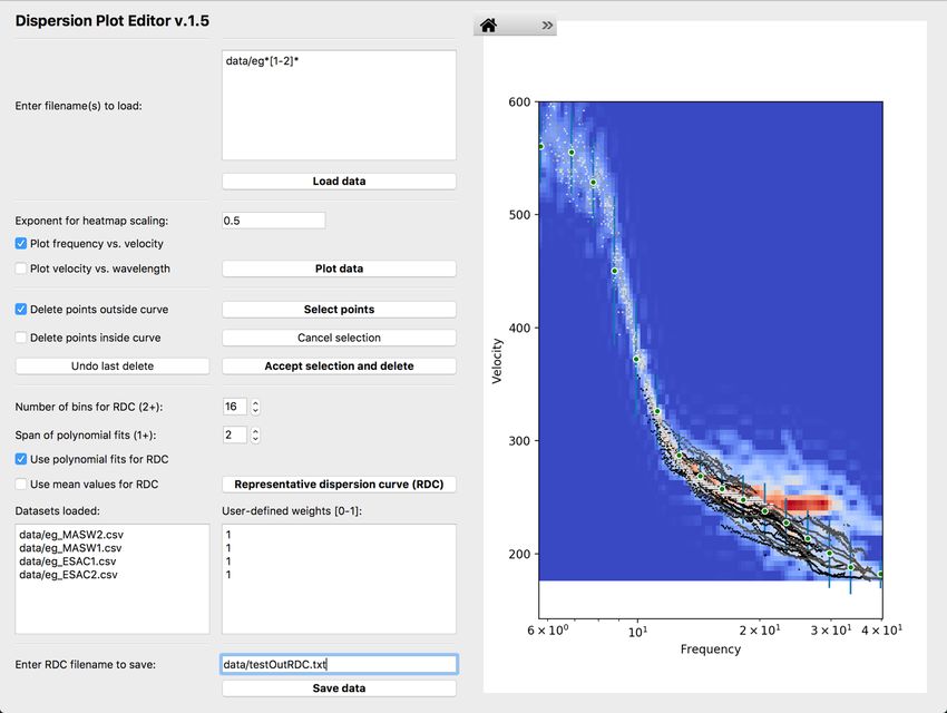
Figure 5. Screenshot showing example of saving data. Enter output filename for the RDC. Save both the RDC and all
edited datasets by clicking on “Save data.”8 Graphical Dispersion Plot Editor (DPE) for Seismic-Site Characterization by Using Multiple Surface-Wave Methods
References Cited Stephenson, W.J., Louie, J.N., Pullammanappallil, S.,
Williams, R.A., and Odum, J.K., 2005, Blind shear-wave
velocity comparison of ReMi and MASW results with
Beyreuther, M., Barsch, R., Krischer, L., Megies, T., Behr, Y., boreholes to 200 m in the Santa Clara Valley—Implications
and Wassermann, J., 2010, ObsPy—A Python Toolbox for for Earthquake Ground Motion Assessment: Bulletin
Seismology: Seismological Research Letters, v. 81, no. 3, of the Seismological Society of America, v. 95, no. 6,
p. 530–533. https://doi.org/10.1785/gssrl.81.3.530. p. 2506–2516. https://doi.org/10.1785/0120040240.
Foti, S., 1999, Multi-station methods for geotechnical Stokoe, K.H., Nazarian, S., Rix, G.J., Sanchez-Salinero, I.,
characterization of surface waves: Ph.D. Dissertation, Sheu, J.C., and Mok, Y.-J., 1988, In situ seismic testing of
Politecnico di Torino. hard-to-sample soils by surface wave method, Proceedings
Haskell, N.A., 1953, The dispersion of surface waves on (Earthquake Engineering and Soil Dynamics II—Recent
multilayered media: Bulletin of the Seismological Society Advances in Ground-Motion Evaluation) of Geotechnical
of America, v. 43, p. 17–34. Engineering Division of the American Society of Civil
Joh, S.H., 1996, Advances in interpretation and analysis Engineers (ASCE), Park City, Utah, 27–30 June 1988:
techniques for spectral-analysis-of-surface-waves (SASW) Geotechnical Special Publication 20, p. 264–278.
measurements: Ph.D. Dissertation, University of Texas Tokimatsu, K., Tamura, S., and Kojima, H., 1992, Effects
at Austin. of multiple modes on Rayleigh wave dispersion
Krischer, L., Megies, T., Barsch, R., Beyreuther, M., Lecocq, characteristics: Journal of Geotechnical Engineering, v. 118,
T., Caudron, C., and Wassermann, J., 2015, ObsPy—A no. 10, p. 1529–1543. https://doi.org/10.1061/(ASCE)0733-
bridge for seismology into the scientific Python ecosystem: 9410(1992)118:10(1529).
Computational Science & Discovery, v. 8, no. 1, p. 014003. Yong, A., Martin, A., Stokoe, K., and Diehl, J., 2013,
https://doi.org/10.1088/1749-4699/8/1/014003. ARRA-funded VS30 measurements using multi-technique
Louie, J.N., 2001, Faster, better—Shear-wave velocity to 100 approach at strong-motion stations in California and
meters depth from refraction microtremor arrays: Bulletin central-eastern United States: U.S. Geological Survey
of the Seismological Society of America, v. 91, no. 2, Open-File Report 2013–1102, 60 p. and data files,
p. 347–364. https://doi.org/10.1785/0120000098. https://pubs.usgs.gov/of/2013/1102/
Martin, A.J., Yong, A., and Salomne, L., 2014, Advantages Yong, A., and COSMOS Guidelines Facilitation Committee,
of active Love wave techniques in geophysical 2016, A progress report on the development of the
characterizations of seismographic stations—Case studies COSMOS International Guidelines for Applying
in California and the central and eastern United States: Noninvasive Geophysical Techniques to Characterize
Proceedings of 10th National Conference on Earthquake Seismic Site Conditions: Proceedings of the 2016 Fall
Engineering, Anchorage, Alaska, 21–25 July 2014, 11 p. Meeting of the American Geophysical Union, Paper
Martin, A., Yong, A., Stephenson, W., Boatwright, J., and No. S43E-05.
Diehl, J., 2017, Geophysical characterization of seismic Yong, A., and COSMOS Guidelines Facilitation Committee,
station sites in the United States—The importance of a 2017, Progress on COSMOS site characterization
flexible, multi-method approach: Proceedings of the 16th guidelines: Proceedings of the 2017 COSMOS Annual
World Conference on Earthquake Engineering, Santiago, Technical Session.
Chile, Jan. 9–13, 2017, Paper No. 2160.
Yong, A., and COSMOS Guidelines Facilitation Committee,
Megies, T., Beyreuther, M., Barsch, R., Krischer, L., and 2018, In memory of Marcos Mucciarelli and his
Wassermann, J., 2011, ObsPy—What can it do for data contributions to the development of the COSMOS
centers and observatories?: Annals of Geophysics, v. 54, International Guidelines for Applying Noninvasive
no. 1, p. 47–58. https://doi.org/10.4401/ag-4838. Geophysical Techniques to Characterize Seismic Site
Okada, H., 2003, The Microtremor Survey Method— Conditions: Proceedings of the 2018 36th European
Geophysical Monograph Series, no.12: Tulsa, Oklahoma, Seismological Commission General Assembly, Valleta,
Society of Exploration Geophysicists, 135 p., https://doi. Malta, 3–7 September, 2018.
org/10.1190/1.9781560801740. Yong, A., Nigbor, R., and Steidl, J., 2018, COSMOS
Park, C.B., Xia, J., and Miller, R.D., 1998, Imaging dispersion Noninvasive Site Characterization Guidelines: Project
curves of surface waves on multi-channel record: Expanded Report: Proceedings of the 2018 COSMOS Annual
Abstracts of 68th Annual International Meeting of the Technical Session, Oakland, California, 16 November.
Society of Exploration Geophysics, p. 1377–1380. Yong, A., McPhillips, D., and Martin, A., 2019, A Graphical
Park, C.B., Miller, R.D., and Xia, J., 1999, Multichannel Dispersion Curve Editing Tool for Seismic Site
analysis of surface waves: Geophysics, v. 64, no. 3, Characterization Using Surface Waves: Seismological
p. 800–808. https://doi.org/10.1190/1.1444590. Research Letters, v. 90, no. 2B, p. 1054.Moffet Field Publishing Service Center, California Manuscript approved for publication May 28, 2020 Edited by Mary Ashman and Aditya S. Navale Layout and design by Kimber Petersen
McPhillips and others—Graphical Dispersion Plot Editor (DPE) for Seismic-Site Characterization by Using Multiple Surface-Wave Methods—OFR 2020–1065
https://doi.org/10.3133/ofr20201065
ISSN 2331-1258 (online)You can also read