Comparing OMI-TOMS and OMI-DOAS total ozone column data
←
→
Page content transcription
If your browser does not render page correctly, please read the page content below
JOURNAL OF GEOPHYSICAL RESEARCH, VOL. 113, D16S28, doi:10.1029/2007JD008798, 2008
  Click
  Here
    for
 Full
Article

Comparing OMI-TOMS and OMI-DOAS total ozone column data
M. Kroon,1 J. P. Veefkind,1 M. Sneep,1 R. D. McPeters,2 P. K. Bhartia,2 and P. F. Levelt1
Received 13 April 2007; revised 18 September 2007; accepted 7 December 2007; published 23 May 2008.

[1] The Ozone Monitoring Instrument (OMI) project team uses two total ozone retrieval
algorithms in order to maintain the long-term record established with Total Ozone
Mapping Spectrometer (TOMS) data as well as to improve the ozone column estimate
using the hyperspectral capability of OMI. The purpose of this study is to assess where
the algorithms produce comparable results and where the differences are significant.
Starting with the same set of Earth reflectance data, the total ozone data used in this study
have been derived using OMI-TOMS and OMI–Differential Optical Absorption
Spectroscopy (DOAS) algorithms. OMI-TOMS is based on the TOMS version 8
algorithm that has been used to process TOMS data taken since November 1978. The
OMI-DOAS retrieval algorithm was developed specifically for OMI. It takes advantage of
the hyperspectral feature of the OMI instrument to reduce errors due to aerosols, clouds,
surface, and sulfur dioxide from volcanic eruptions. The OMI-DOAS algorithm also
has improved correction for cloud height. The mean differences in the ozone column
derived from the two algorithms vary from 0 to 9 DU (0–3%), and their correlation
coefficients vary between 0.89 and 0.99 with latitude and season. The largest differences
occur in the polar regions and over clouds. Some of the differences are due to stray light,
dark current, and other instrumental errors that have been corrected in the new version
of the OMI radiance/irradiance data set (collection 3). Other differences are algorithmic.
OMI-DOAS algorithmic errors identified through this analysis are also being corrected in
collection 3 reprocessing. However, for consistency with the long-term TOMS record,
OMI-TOMS collection 3 data will still be based on the TOMS V8 algorithm. Preliminary
analysis shows much better agreement in the two total ozone data sets after reprocessing.
Reprocessed collection 3 data from both algorithms will be available before the end of
2007. Continuing the TOMS total ozone column data record that dates back to November
1978 is the primary OMI mission goal that is achievable with either OMI total ozone
column data product.
Citation: Kroon, M., J. P. Veefkind, M. Sneep, R. D. McPeters, P. K. Bhartia, and P. F. Levelt (2008), Comparing OMI-TOMS and
OMI-DOAS total ozone column data, J. Geophys. Res., 113, D16S28, doi:10.1029/2007JD008798.

1. Introduction                                                                OMI–Differential Optical Absorption Spectroscopy (DOAS)
                                                                               [Bhartia and Wellemeyer, 2002; Veefkind et al., 2006]
  [2] The Dutch-Finnish Ozone Monitoring Instrument                            and OMI-Total Ozone Mapping Spectrometer (TOMS)
(OMI) [Levelt et al., 2006a, 2006b] aboard the NASA Earth                      [Bhartia and Wellemeyer, 2002; Balis et el., 2007;
Observing System (EOS) Aura satellite [Schoeberl et al.,                       McPeters et al., 2008] total ozone column retrieval
2006] is a compact nadir viewing, wide swath, ultraviolet-                     algorithms. (Please read the README files of these data
visible (270– 500 nm) hyperspectral imaging spectrometer                       product carefully prior to use. OMI README files are
that provides daily global coverage with high spatial and                      available at http://disc.gsfc.nasa.gov/Aura/OMI/.) The
spectral resolution. The Aura orbit is Sun-synchronous at                      OMI-TOMS algorithm is based on the TOMS V8 algorithm
705 km altitude with a 98° inclination and ascending node                      that has been used to process data from a series of four TOMS
equator-crossing time roughly at 1345 local time (LT). OMI                     instruments flown since November 1978. This algorithm uses
measures backscattered solar radiance in the dayside portion                   measurements at 4 discrete 1 nm wide wavelength bands
of each orbit and solar irradiance near the Northern Hemi-                     centered at 313, 318, 331 and 360 nm. The OMI-DOAS
sphere terminator once per day. The OMI data products                          algorithm [Veefkind et al., 2006] takes advantage of the
are derived from the ratio of Earth radiance and solar                         hyperspectral feature of OMI. It is based on the principle of
irradiance. In this paper we compare the output of the                         Differential Optical Absorption Spectroscopy (DOAS)
   1
                                                                               [Perner and Platt, 1979]. The algorithm uses 25 OMI
       Royal Netherlands Meteorological Institute, De Bilt, Netherlands.       measurements in the wavelength range 331.1 nm to
   2
       NASA Goddard Space Flight Center, Greenbelt, Maryland, USA.
                                                                               336.6 nm, as described by Veefkind et al. [2006]. The key
Copyright 2008 by the American Geophysical Union.                              difference between the two algorithms is that the DOAS
0148-0227/08/2007JD008798$09.00                                                algorithm removes the effects of aerosols, clouds, volcanic

                                                                           D16S28                                                    1 of 17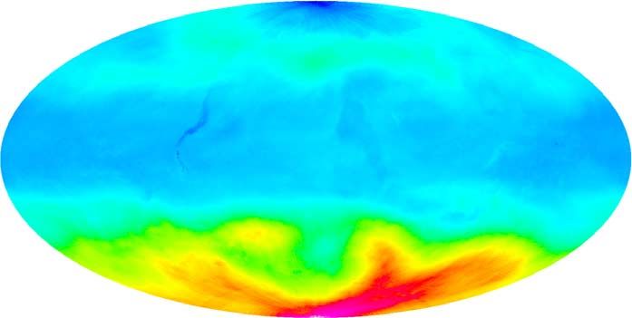
D16S28 KROON ET AL.: COMPARING OMI-TOMS AND OMI-DOAS OZONE D16S28
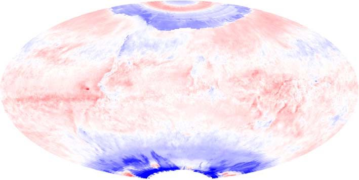
Figure 1. Global distribution of Ozone Monitoring Instrument – Total Ozone Mapping Spectrometer
(OMI-TOMS) total column ozone expressed in Dobson units regridded to a 180 360 grid (1.0° 1.0°
resolution). The data are from the time period 21– 27 March 2005, and are presented in the Mollweide
projection and polar top views. Note the large dynamical range of total ozone columns over the globe.
sulfur dioxide, and surface effects by spectral fitting while geometry, and as a function of atmospheric quantities
the TOMS algorithm applies an empirical correction to measured over the same ground pixel.
remove these effects. In addition, the TOMS algorithm uses
a cloud height climatology that was derived using infrared 2. Data and Analysis
satellite data, while the DOAS algorithm uses cloud informa-
tion derived from OMI measurements in the 470 nm O2-O2 [3] OMI level 2 data comes in the form of orbit files that
absorption band. The two algorithms also respond to contain trace gas abundances as retrieved on the day side of
instrumental errors very differently. The purpose of this the Aura orbit from the level 1B reflectance spectra. OMI
study is to assess the quality of the OMI-DOAS and level 2 data products used in this study are OMI-DOAS
OMI-TOMS total ozone column data product by their total ozone column, labeled OMDOAO3; OMI-TOMS total
similarities and their differences, and to associate these ozone column, labeled OMTO3; and OMI total sulfur
differences with particular characteristics of the retrievals. dioxide column, labeled OMSO2. The data were obtained
We first compare global images of the total ozone columns from the OMI Science Investigator-led Processing System
from the two algorithms to check whether they render the (OSIPS) of Earth Observing System Data and Information
same patterns and structures. We then look more quantita- System Core System (ECS) collection 2. The time period
tively at the correlation and proportionality between the two covered is from September 2004 to June 2007. From the
data sets. We report differences between OMI-TOMS and start of the OMI data record, the results of validation
OMI-DOAS total ozone columns in global images, as a exercises have been used to identify OMI-DOAS algorithm
function of various parameters describing the measurements shortcomings and to provide insights into where retrieval
algorithm improvements were needed. The implementation
2 of 17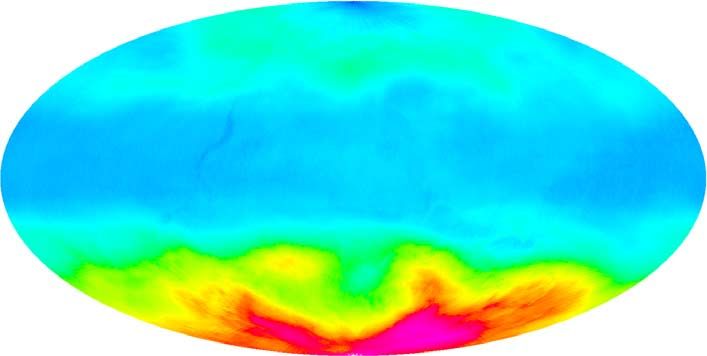
D16S28                      KROON ET AL.: COMPARING OMI-TOMS AND OMI-DOAS OZONE                                     D16S28

         Figure 2. Global distribution of OMI –Differential Optical Absorption Spectroscopy (DOAS) total
         column ozone expressed in Dobson units regridded to a 180  360 grid (1.0°  1.0° resolution). The data
         are from the time period 21– 27 March 2005, and are presented in the Mollweide projection and polar top
         views. Note the structures similar to those presented in Figure 1.

of these improvements has resulted in the release of a           by a range of orbit numbers, and per orbit file read a set
number of versions of the software. Data collected between       of data fields. Data is filtered synchronously on the basis
September 2004 and October 2005 was processed with               of the values of quality flags and limits set. Synchronous
software version v0.9.4. From October 2005 onward                filtering of the data fields in OMI orbit data means that
v1.0.1 has been operational. The absolute differences be-        when the value of a certain data field does not pass the
tween these versions are minor, much smaller than the            filter conditions imposed, that pixel position is filled
retrieval accuracy. Therefore we consider the OMI-DOAS           with a Not-A-Number value in all data fields to be
data record as continuous. At the time of writing, the further   ignored by the subsequent calculations. The CAMA
optimized OMI-DOAS algorithm is ready for reprocessing           toolbox allows not only exploration of a single OMI
the OMI data record into collection 3.                           data product, for example OMI-DOAS total ozone col-
  [4] Data analysis is performed with the CAMA toolbox           umn and its cloud fraction, and the relation between
written by Maarten Sneep of KNMI (CAMA, 2006: For                these data fields, but also the exploration of interdepen-
more information, please visit our Web site, http://             dencies of two or more OMI data products, for example
www.knmi.nl/omi/research/validation/cama/, where the             OMI-DOAS and OMI-TOMS, and the correlation of
CAMA software can be downloaded and documentation                their differences with respect to, e.g., cloud fraction,
can be obtained. CAMA runs under IDL.). CAMA                     cloud pressure, snow/ice coverage and other OMI trace
stands for ‘‘Correleer Alles Met Alles,’’ literally meaning      gases. The toolbox performs a statistical analysis of all
‘‘correlate everything with everything.’’ This toolbox can       read quantities and preinstructed derivatives per ground
be instructed to read an OMI level 2 data set described          pixel, yielding frequency distributions and along-track

                                                            3 of 17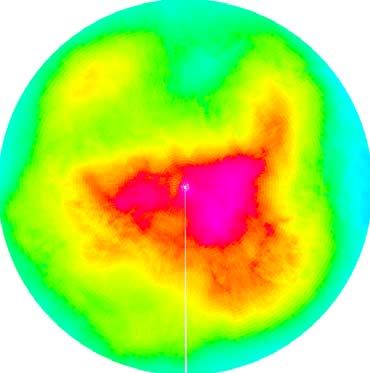
D16S28                     KROON ET AL.: COMPARING OMI-TOMS AND OMI-DOAS OZONE                                       D16S28

         Figure 3. Graphical representation of the OMI total ozone column data products versus time (from top
         to bottom) as averaged over the whole globe, the Northern Hemisphere, and the Southern Hemisphere.
         Note the 2006 record ozone hole significantly lowering globally averaged ozone. Please note the different
         dynamic range for all three plots.

                                                          4 of 17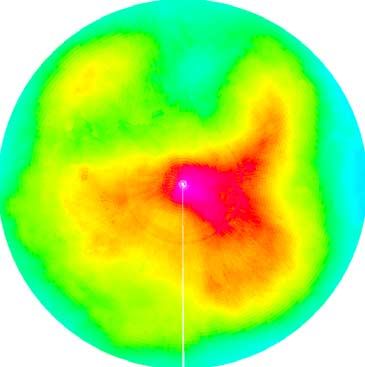
D16S28                    KROON ET AL.: COMPARING OMI-TOMS AND OMI-DOAS OZONE                                   D16S28

         Figure 4. Graphical representation of the correlation and regression coefficient of OMI-TOMS and
         OMI-DOAS total ozone column versus time for (from top to bottom), the whole globe, the Northern and
         Southern hemispheres. Note the high degree of correlation and proportionality between both OMI total
         ozone data products over the entire data record.

                                                       5 of 17
D16S28                   KROON ET AL.: COMPARING OMI-TOMS AND OMI-DOAS OZONE                               D16S28

         Figure 5. Graphical representation of the standard deviation of the OMI-TOMS and OMI-DOAS total
         ozone column versus time for (from top to bottom), the whole globe, the Northern and Southern
         hemispheres.

                                                     6 of 17
D16S28                    KROON ET AL.: COMPARING OMI-TOMS AND OMI-DOAS OZONE                                    D16S28

                                                             total ozone columns, regional comparisons have been
                                                             made incorporating OMI data zoomed into a region of
                                                             interest near volcanic eruptions. Such an approach
                                                             reveals the strong local effects of these emissions which
                                                             are otherwise obscured by global statistics. In addition,
                                                             the CAMA toolbox calculates global distributions of all
                                                             read quantities by means of regridding to a latitude-
                                                             longitude grid with a resolution predefined by the user
                                                             yielding, e.g., global images of OMI-DOAS and OMI-
                                                             TOMS total ozone columns and their differences. The
                                                             regridding is performed by averaging all OMI data
                                                             points for which the pixel center coordinates fall within
                                                             that particular grid cell. Because regridded data is used
                                                             here for visualization purposes only, no advanced weigh-
                                                             ing is applied. The global images obtained reveal the
                                                             global structures of the read data sets and those features
                                                             that depend on geography.

                                                             3. Global Distributions of Total Ozone Column
                                                              [5] Figures 1 and 2 show the global distribution of
                                                             OMI-TOMS and OMI-DOAS total ozone column, respec-

Figure 6. Logarithmic (base 10) scatter density plots of
OMI-TOMS versus OMI-DOAS total ozone columns in the
Northern Hemisphere for the time period 14 to 20
December 2004 (top) and in the Southern Hemisphere for
the time period 14 to 20 September 2005 (bottom). Note the
bimodal distribution in the Southern Hemisphere data
during the occurrence of the ozone hole.

averages of the individual quantities. The toolbox also
calculates scatter density plots, and tables describing      Figure 7. Global along-track averages of total ozone
statistical averages and standard deviations, correlation    column for OMI-TOMS (top) and OMI-DOAS (bottom) for
and covariance coefficients, skewness and kurtosis coef-     the time period 14 to 27 March 2006 of OMI cross track
ficients, and regression coefficients for all combinations   positions. In these graphs the middle line denotes the total
of parameters. These analyses have been performed for        ozone column averaged over the time period mentioned for
the whole globe and for the Northern and Southern            each OMI track position, ranging from 1 to 60, individually.
hemispheres separately to study the different behavior       The lines above and below the mean denote the mean plus
of OMI data products in both hemispheres. To study the       or minus one standard deviation for each ground pixel
effect of volcanic emissions of sulfur dioxide on OMI        individually.

                                                        7 of 17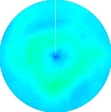
D16S28                      KROON ET AL.: COMPARING OMI-TOMS AND OMI-DOAS OZONE                                        D16S28

         Figure 8. Global distribution of OMI-TOMS and OMI-DOAS total column ozone difference expressed
         in Dobson units regridded to a 180  360 grid (1.0°  1.0° resolution). The data are from the time period
         14 to 27 October 2005, and are presented in the Mollweide projection and polar top views. Note the
         visibility of sea ice structures around Antarctica, the dark blue structures at the high latitudes in the
         Northern Hemisphere and a volcanic eruption at the Galapagos Islands in the east Pacific Ocean.

tively. Each image is obtained by regridding OMI data for        0 – 8 DU less total ozone column than OMI-DOAS,
the time period 21 to 27 March 2005, consisting of 102           depending on the season. Differences are largest during
orbits, to a latitude-longitude grid of 1.0°  1.0° resolution   late spring (May) and early summer (June). The record
(180  360). A comparison of Figures 1 and 2 reveals             breaking 2006 ozone hole significantly lowered globally
very similar structures in OMI-TOMS and OMI-DOAS                 averaged ozone in the SH spring of 2006. Figure 3 shows
total ozone columns. There are no obvious geographical           that both OMI-TOMS and OMI-DOAS hemispheric
dependencies observed. Results for other time periods look       averages show a similar annual cycle of 40 DU (NH) and
very similar.                                                    20 DU (SH) amplitude. More obviously, there is a 6 month
  [6] Figures 3, 4, and 5 provide a statistical comparison of    phase shift between the two hemispheres, but the timing of
OMI-TOMS and OMI-DOAS total column ozone data                    the minima/maxima in the SH is erratic and is strongly
during the time period September 2004 to June 2007.              affected (presumably) by interannually varying ozone hole
Results are reported separately for the whole globe and          effects.
for the Northern (NH) and Southern (SH) hemispheres for            [7] Figure 4 show that both total ozone data products
days 14 to 27 of each month. These time intervals are            correlate well over the OMI data record; the correlation
centered on the equinox and solstice dates. Figure 3 shows       coefficients range from 0.89 to 0.99, depending on season.
that globally averaged OMI-TOMS and OMI-DOAS total               The regression coefficients range from 0.87 to unity, which
ozone columns are in close agreement over the OMI data           shows that the two data sets vary linearly against each other.
record and show a similar annual cycle of 25 – 30 DU             The near unity regression and correlation in the Southern
amplitude. On the global scale, OMI-TOMS reports                 Hemisphere during the ozone hole season indicates good

                                                            8 of 17
D16S28 KROON ET AL.: COMPARING OMI-TOMS AND OMI-DOAS OZONE D16S28
Figure 9. Graphical representation of the total ozone column difference (OMI-TOMS minus OMI
DOAS) and its standard deviation versus time for (from top to bottom), the whole globe, the Northern
and Southern hemispheres.
9 of 17D16S28 KROON ET AL.: COMPARING OMI-TOMS AND OMI-DOAS OZONE D16S28
agreement between the two data sets over a wide range of
total column values where minimum columns reach below
100 DU. In the Northern Hemisphere their different
behavior, particularly over snow and ice, reduced the
regression coefficient.
[8] The regression coefficient is the correlation coeffi-
cient multiplied by the ratio of the standard deviations of
the two total ozone columns. This statement follows
directly from using the matrix elements of the covariance
matrix for calculating these quantities. Given the high
correlations coefficients, additional information supplied
by the regression coefficient is the ratio of these standard
deviations which are physical measures of the natural
variability of the total ozone column. On average
Figure 4 indicates that OMI-TOMS ozone is varying to
some extent less than OMI-DOAS ozone. This observation
is exemplified by Figure 5 which shows that the standard
deviation of the OMI-TOMS and OMI-DOAS total ozone
column for the OMI data record are in close agreement
even though both fluctuate strongly depending on season.
The natural variability on both hemispheres runs approxi-
mately half a year out of phase, and is dominated on the
Southern Hemisphere by the variability of the ozone hole.
[9] In Figure 6 we show the scatter density plots of
OMI-TOMS versus OMI-DOAS total ozone column on a
logarithmic (base 10) color scale for two different time
periods for the Northern and Southern hemispheres. Scatter
densities represent the statistical occurrence of pairs of values
from both axis. The strong correlation between OMI-TOMS
and OMI-DOAS total ozone columns in both hemispheres is
evident from the graphs. In the Southern Hemisphere the
correlation is as pronounced as in the Northern Hemisphere,
although covering a smaller dynamic range during most of
the year. During the Southern Hemisphere ozone hole season,
from September to December, the statistics for the Southern
Hemisphere appear to become bimodal with the collection of
data points in the lower left corner associated with the ozone
hole. The observation of this bimodal distribution highlights
the extreme conditions of the ozone hole. There are almost no
total ozone column observations between 200 and 230 DU
indicating that entering the vortex represents a dramatic
transition from normal ozone conditions to extremely low
ozone conditions, even when resolved by OMI. The signature
of the bimodal distribution is strongest when the ozone hole is
deepest and weakens as the meteorological polar vortex
weakens with the arrival of local spring.
[10] The OMI ground swath of 2600 km wide is divided
into 60 ground pixels, where positions 29, 30 denote the
exact subsatellite positions [Levelt, 2002]. All OMI data
products are retrieved at each pixel ground location, although
the optical measurement geometry, described by the solar and
viewing azimuth and zenith angles, varies strongly over the
swath. However, the OMI retrieval algorithms are expected
to determine the abundance of atmospheric trace gases
irrespective of the optical measurement geometry irrespec-
Figure 10. OMI-TOMS (top) and OMI-DOAS (middle)
total ozone column and their difference (bottom) over the
Northern Hemisphere for a single orbit 3625 recorded on
21 March 2005. Note the presence of a strong stepwise
change ranging beyond 30 DU (or 10%) in OMI-TOMS
that is absent in OMI-DOAS.
10 of 17D16S28 KROON ET AL.: COMPARING OMI-TOMS AND OMI-DOAS OZONE D16S28
(OMI-TOMS minus OMI-DOAS). This image was gener-
ated using a week of data from the time period 14 to
27 October 2005, regridded to a latitude-longitude grid of
1.0° 1.0° resolution (180 360). Figure 8 reveals (1) the
eruption of the Sierra Negra volcano in the east Pacific
Ocean, Galapagos Islands, (2) a clear indication of the
dependence on Antarctic sea ice, (3) significant differences
in the northern high latitudes, and (4) and a ring-shaped
feature near 85°S, the diameter of which expands as the Sun
rises over the South Pole. The features observed in the
global total column ozone difference images vary signifi-
cantly as a function of season, being influenced by surface
albedo, snow and ice coverage, clouds, OMI observing
angles, the position of the orbit terminators and episodic
events such as volcanic eruptions.
[12] Figure 9 provides the total ozone column difference
and its standard deviation for the OMI data record for the
whole globe and for the Northern and Southern hemispheres
separately. On the global scale, OMI-DOAS reports 0 – 8 DU
more total ozone column than OMI-TOMS, depending on
the season. Differences are largest during late spring (May)
and early summer (June). The standard deviation of the total
ozone column difference is considerably smaller than the
standard deviation of the total ozone columns alone and also
depends on the season. The Northern Hemisphere clearly
dominates the global behavior of the total ozone column
difference while the Southern Hemisphere shows tranquil
behavior with time.
[13] Images constructed from regridded total column
ozone difference data reveal the presence of various ring-
shaped features at the high latitudes in the Northern and
Southern hemispheres. To investigate the origin of these
features, individual orbits have been analyzed. Figure 10
shows the OMI-TOMS and OMI-DOAS total ozone column
in the Northern Hemisphere for a single orbit 3625 recorded
on 21 March 2005. In this image OMI-TOMS shows a
discontinuity which is absent in OMI-DOAS. Figure 10 also
shows that the discontinuity can exceed 40 DU. This
discontinuity occurs at 70° solar zenith angle where the
TOMS V8 algorithm starts to use 313 nm measurements to
correct for errors due to variations in ozone profile from
climatology. Recent results indicate that a large part of this
discontinuity is caused by stray light caused errors in the
Figure 11. Logarithmic (base 10) scatter density plots of OMI measurements at 313 nm. It will be corrected when the
the solar zenith angle versus the total ozone column OMI data are reprocessed using collection 3. However,
difference for the time period 14 to 20 December 2004 smaller discontinuities are also present in the TOMS data;
for the Northern (top) and Southern (bottom) hemispheres. they could be due to relative errors in laboratory measured
ozone cross sections or some other unknown cause. The
tive of the OMI cross track position. The CAMA toolbox ring-like feature closer to the terminator has been identified
generates along-track averages of all cross-track positions as error in the calculation of the air mass factor in the
of the read data fields to check this assumption. Examples OMI-DOAS algorithm largely due to an erroneous correction
of global along-track averages for OMI-TOMS and for the spherical atmosphere.
OMI-DOAS total ozone columns are shown in Figure 7.
From these graphs available for the OMI data record we 5. Solar Zenith Angle
conclude that the OMI total column ozone data products are
[14] In Figure 11 we present scatter density plots of the
independent of swath position.
solar zenith angle versus the total ozone column difference.
These graphs again reveal the presence of a discontinuity at
4. Global Distributions of Total Ozone Column 70° solar zenith angle. Beyond 70° solar zenith angle the
Difference differences vary strongly as a function of solar zenith angle
[11] Figure 8 shows the global distribution of the OMI with the strong swing to high values close to 87° being
total ozone column differences, in this paper calculated as caused by the error in the OMI-DOAS air mass factor. In
11 of 17D16S28 KROON ET AL.: COMPARING OMI-TOMS AND OMI-DOAS OZONE D16S28
Figure 12. Single orbit plots for OMI orbit 8940 over topical regions recorded on 21 March 2006 of the
OMI-TOMS (top left) and OMI-DOAS (bottom left) total ozone columns, OMI-DOAS cloud fraction
(top right) and OMI total ozone column difference (bottom right). Note the similarities of small-scale
structures observed in the total ozone column difference with the cloud fraction and the OMI-TOMS
total ozone field, where the dynamic range of the ozone field plots has been adjusted to enhance the
observed cloud structures.
addition, there is also a steady trend in the total ozone These solutions will be incorporated in reprocessing the
column difference over the range 30° –70° in solar zenith OMI-DOAS data record into collection 3.
angle, being caused by the same shortcoming. In summary,
this particular plot reveals several algorithm features that 6. Clouds
deserve improvements. At the time of writing new air mass
factor tables have been calculated for OMI-DOAS on the [15] Plotting total ozone columns for single OMI orbits
basis of improved radiative transfer calculations. These over tropical regions reveals the presence of small-scale
improvements include a method to specifically deal with structures in OMI-TOMS data which appear to be absent in
elastic (Cabannes) and inelastic (Cabannes) scattering. OMI-DOAS data. Figure 12 shows single orbit plots for
OMI data products for orbit 8940 over topical regions
12 of 17D16S28 KROON ET AL.: COMPARING OMI-TOMS AND OMI-DOAS OZONE D16S28
clear correlation with the difference in the cloud pressure
assumed by the two algorithms, as shown in Figure 13.
[16] The OMI-TOMS algorithm uses a cloud top pressure
climatology that was derived from a thermal infrared (TIR)
sensor (THIR) that flew on the Nimbus-7 satellite in the
1980s. In deriving this climatology only bright clouds were
used to avoid biasing the results by thin cirrus that have
virtually no effect on UV but affect TIR significantly. This
information is used by the TOMS algorithm to correct the
OMI radiances for the Ring Effect, for the O2-O2 absorption
at 360 nm, for enhanced ozone absorption above clouds due
to multiple scattering, and for reduced absorption below
clouds. By happenstance all these effects are of the same
sign at wavelengths used in the TOMS V8 algorithm,
making this algorithm more sensitive to error in cloud
height than if some other wavelengths had been used
in designing the TOMS instrument. In addition, the
OMI-DOAS algorithm uses an effective cloud pressure
estimated from the OMI data itself using the 470 nm O2-O2
absorption band. These cloud pressures are on the average
200 – 300 hPa larger that those reported by TIR sensors
(Figure 13). This difference is caused by the fact that the
outgoing radiation at the UV/Visible wavelengths is less
sensitive to ice clouds than at TIR wavelengths, and thus
OMI more often sees the lower-level water clouds.
OMI-TOMS data processed using O2-O2 derived cloud
pressures produce essentially the same results over clouds as
does OMI-DOAS. Since we believe that OMI-derived ef-
fective cloud pressures are more appropriate for analyzing
UV/Visible radiance data than those provided by TIR
sensors, the next version of the TOMS algorithm will be
based on cloud effective pressure climatology derived from
OMI, rather than TIR-derived cloud top pressures.
7. Striping Features
[17] Zooming in on the dynamic range of ozone columns
in the tropics actually enhances the appearance of the
striping features as observed in the OMI-DOAS total ozone
column plots of Figure 12. The largest contribution to these
stripes is caused by insufficient dark current correction of
the solar irradiance measurements. The dark current varia-
tions are picked up by the OMI CCD detectors when they
Figure 13. Logarithmic (base 10) scatter density plots of are hit by cosmic radiation. In the ECS collection 2 data,
the OMI-TOMS and OMI-DOAS cloud pressure difference on which this paper is based, the dark current was
versus the OMI-DOAS cloud pressure (top) and versus the assumed to be constant over several weeks, however, this
OMI-TOMS and OMI-DOAS total ozone column difference turned out not be sufficient. For the collection 3, the dark
(bottom). Correlation coefficients are R = 0.79 and R = current maps will be updated on a daily basis, which is
0.67 for Figure 13 top and bottom, respectively. expected to give much better results [Dobber et al., 2008].
The reason that the OMI-DOAS total ozone shows more
recorded on 21 March 2006. The similarities of small-scale stripes than the OMI-TOMS data is because the DOAS
structures observed in the total ozone column difference implementation is using smaller variations in the ozone
with the cloud fraction and the OMI-TOMS total ozone field absorption which are more strongly affected by the dark
led to investigating the correlation of total ozone column data current than are the OMI-TOMS bands. In addition, for
with cloud fraction and pressure. No significant correlations OMI-TOMS correction techniques known as ‘‘soft calibra-
were found between total ozone column data and cloud tion’’ are applied as a function of cross track position that very
fraction and cloud top pressure data. Furthermore, the OMI effectively reduce striping. Soft calibration is based on the
total ozone column difference showed no correlation with principle that wavelength-dependent calibration can be in-
OMI-TOMS or OMI-DOAS cloud fraction or their cloud ferred from the requirement that ozone derived at different
fraction difference. For cloud fractions lower than 5%, wavelengths must be consistent. For OMI-DOAS in the ECS
OMI-TOMS and OMI-DOAS total ozone columns are collection 2 starting with software version 1.0.1 from October
similar down to the 1.0 DU level. However, there is a 2005 onward, a fixed irradiance is used, which has been
13 of 17D16S28 KROON ET AL.: COMPARING OMI-TOMS AND OMI-DOAS OZONE D16S28
Figure 15. Logarithmic (base 10) scatter density plots of
the OMI-SO2 15 km total sulfur dioxide column versus the
difference of OMI-TOMS and OMI-DOAS total ozone
columns for the region around the volcano Sierra Negra on
Isla Isabelle. The structures and dependence of OMI-TOMS
on the total sulfur dioxide column propagate into this graph.
Sierra Negra on the Galapagos Islands and Anatahan in
the Mariana Archipelago. The exact moment of volcanic
eruptions can be retrieved from the Earth Observatory Web
site where OMI observations from the sulfur dioxide (SO2)
data product [Carn et al., 2007] are regularly posted (August
2005: Anatahan, Mariana Islands, United States, available at
http://earthobservatory.nasa.gov/NaturalHazards/natural_
hazards_v2.php3?img_id=13043; October 2005: Sierra
Negra, Galapagos Islands, Ecuador, available at http://
earthobservatory.nasa.gov/NaturalHazards/natural_hazards_
v2.php3?img_id=13253). The occurrence of large values in
certain regions of global images of the OMI total ozone
column difference seems to temporally and spatially coin-
cide with these volcanic eruptions, an example of which is
shown in Figure 8. A strongly positive and irregularly
Figure 14. Logarithmic (base 10) scatter density plots of shaped feature appears in the east Pacific Ocean near the
the OMI-SO2 15 km total sulfur dioxide column versus Galapagos Islands around the time of the main eruption. The
OMI-TOMS (top) and OMI-DOAS (bottom) total ozone reasoning above leads us to believe that volcanic eruptions
columns for the region around the volcano Sierra Negra on are visible in the OMI total ozone column difference.
Isla Isabelle. Note the strong dependence of OMI-TOMS on
the total sulfur dioxide column and the absence of this Table 1. Statistical Correlations of OMI Total Ozone Column and
dependence for OMI-DOAS. Total Sulfur Dioxide Column Data Products for the Selected
Region Around the Sierra Negra Volcano for the Time Period 21 to
derived from many irradiance measurements using a median 31 October 2005a
filter. This approach also was a great improvement for reducing OMI-SO2,
the striping features. The absolute differences in total ozone OMI-DOAS OMI-TOMS Delta-O3 15 km
column values between these approaches are minor, much OMI-DOAS 1.00 0.0132 0.395 0.0540
smaller than the retrieval accuracy, by which we consider the OMI-TOMS 0.0132 1.00 0.924 0.663
OMI-DOAS data record as continuous. Delta-O3 0.395 0.924 1.00 0.628
OMI-SO2, 15 km 0.0540 0.663 0.628 1.00
a
Here Delta-O3 denotes total ozone column difference calculated as
8. Volcanic Eruptions Ozone Monitoring Instrument – Total Ozone Mapping Spectrometer (OMI-
[18] During the OMI data record time period several TOMS)/OMI – Differential Optical Absorption Spectroscopy (DOAS). Note
the similar high correlation of OMI-TOMS and Delta-O3 with the OMI-SO2
volcanoes erupted explosively such as Mount Etna in Italy, data products, where OMI-DOAS does not correlate well at all.
14 of 17D16S28 KROON ET AL.: COMPARING OMI-TOMS AND OMI-DOAS OZONE D16S28
oxides, sulfur oxides, hydrogen chloride and halogen gases
(fluorine, chlorine). Here we focus on examining the
correlation between the observed features in the OMI total
ozone column difference plots and the total sulfur dioxide
column, an OMI data product [Carn et al., 2007]. The
correlation with aerosols will be established once the OMI
aerosol data products are validated.
[20] Our case study involves the eruption of the Sierra
Negra volcano on Isla Isabella, Galapagos, Ecuador, in the
time period 21 to 31 October 2005. Calculations were
limited to a region around the volcanic island covering
the range 4.66°S to 3.00°N in latitude and 100.5°W to
87.8°W in longitude, to highlight this localized effect
otherwise obscured in the global average. We computed
statistical correlations between OMI-TOMS, OMI-DOAS,
OMI total ozone column difference and OMI total sulfur
dioxide columns. The OMI-SO2 data product contains
estimates of the total sulfur dioxide columns assuming three
different altitude ranges where sulfur dioxide could reside in
the atmosphere. In view of the explosive nature of the Sierra
Negra volcano, the OMI-SO2 15 km data are considered in
this case study. OMI-TOMS total ozone column data were
filtered for the flag ‘‘quality flags’’ that denotes possible
contamination with sulfur dioxide when set to a value of
‘‘5’’, the binary code 101 of the lowest three bits.
[21] Figure 14 shows the scatter density plot of the OMI-
SO2 15 km total sulfur dioxide column versus OMI-TOMS
and OMI-DOAS total ozone columns for the region and
time period of interest. The OMI-TOMS total column ozone
plot reveals a strong dependence of total column ozone on
the total sulfur dioxide column where OMI-DOAS does not.
OMI-TOMS total ozone column is found to correlate well
with the sulfur dioxide column as does the OMI total ozone
difference, as seen from Figure 15, where OMI-DOAS does
not. Finally, the values of the correlation coefficients
presented in Table 1 support these observations. Values
beyond 0.65 for OMI-TOMS and close to zero for
OMI-DOAS lead to conclude that the effect can be
attributed to OMI-TOMS. Most probably the OMI-TOMS
total ozone column retrieval algorithm does not adequately
distinguish between strong absorption features of ozone or
sulfur dioxide because of the use of selective wavelength
Figure 16. Logarithmic (base 10) scatter density plot of the bands where these features coincide. This is a known fact
solar zenith angle versus the total ozone column difference for older ground based Dobson instruments as well [De
for the time period 13 to 15 January 2006 for the whole globe, Muer and De Backer, 1994]. Enhanced concentrations of
incorporating the new (top) and operational (bottom) sulfur dioxide are represented as enhanced concentrations
OMI-DOAS data product. Here DOAS(col3) denotes the of ozone because the absorption features of both molecules
latest OMI-DOAS algorithm version ready for collection 3 fall in the wavelength range over which the instruments
reprocessing. DOAS(ecs2) and TOMS(ecs2) denote the perform an integration of the measured intensities. The
operational OMI-DOAS and OMI-TOMS data. Note the OMI-DOAS retrieval algorithm on the other hand uses the
reduction of the dramatic swing above 70° SZA as observed OMI spectral resolution to its fullest to distinguish be-
in collection 2. tween the spectral signatures of ozone and sulfur dioxide
In fact, the region where OMI derives ozone is at a
[19] Volcanic eruptions are often accompanied by emis- minimum in the sulfur dioxide spectrum and in that region
sions of large amounts of debris and volatiles. Volcanic there is comparatively little structure.
debris consists of (1) lapilli, blocks and bombs, particles
typically larger than 5 mm that are quickly deposited near 9. Outlook to OMI Collection 3 Total Ozone
the vent, and (2) ash particles (D16S28 KROON ET AL.: COMPARING OMI-TOMS AND OMI-DOAS OZONE D16S28
tions, the OMI calibration team has delivered a data set of difference in sensitivity of the two cloud algorithms to ice
optimal parameter choices of the entire OMI data record clouds.
[Dobber et al., 2008]. With this data set all OMI Level-0 [26] The OMI-TOMS total ozone retrieval algorithm
data will be reprocessed toward a new collection of OMI shows a discontinuity at 70° solar zenith angle. This
level 1B data and subsequent to OMI level 2 data that will appears to be largely, though not entirely, due to OMI
be labeled collection 3. Major improvements of this level stray light effects that will be corrected in collection 3
1B collection are (1) sophisticated and optimized radiomet- reprocessing. Near the terminator the OMI-DOAS algorithm
ric calibration, (2) improved dark current corrections, and underestimates the total ozone column by more than 30 DU
(3) improved stray light corrections. In addition, the level 2 as compared to the OMI-TOMS total ozone retrieval
retrieval algorithms will be optimized on the basis of algorithm. This behavior is now understood and will also
validation results obtained with collection 2. For the be corrected during reprocessing. Preliminary results
OMI-DOAS total ozone column retrieval the most important indicate that the reprocessing will bring the two algorithms
changes are (1) a new air mass factor table to incorporate the in much better agreement.
spherical shape of the atmosphere and (2) a new scheme to [27] The OMI-TOMS retrieval algorithm, based on the
deal with snow and ice covered surfaces. As part of testing TOMS V8 algorithm, appears to be a robust algorithm.
these new developments, OMI-DOAS total ozone column Most of the cloud related errors appear correctable using a
collection 3 data were calculated for various time periods cloud climatology developed using OMI data. Differences
along the OMI data record. In Figure 16 we present between climatology and actual cloud pressures will pro-
preliminary results of comparing OMI-DOAS collections duce a 1 – 2% random noise in OMI-TOMS data. Analysis
3 against OMI-TOMS of collection 2 used as the baseline. shows that the 70° discontinuity problem can be minimized
The solar zenith angle dependence in the range of by selecting the algorithm switching point on the basis of
30° – 70° solar zenith angle has been significantly sup- slant ozone column rather than on solar zenith angle. The
pressed. More importantly, the improved air mass factor next version of the OMI-DOAS retrieval algorithm used in
calculations for OMI-DOAS has removed the dramatic swing collection 3 reprocessing appears to be doing at least as well
around 85°. Results obtained with polar-AVE data and as OMI-TOMS under most conditions and is clearly better
OMI-DOAS collection 3 data have also shown that over under certain conditions, e.g., in presence of volcanic SO2.
bright snow covered surfaces at very high solar zenith Similar analysis of reprocessed data from both algorithms
angle, OMI-DOAS is performing as well as OMI-TOMS will be conducted to identify any remaining weaknesses in
[Kroon et al., 2008]. Please note that OMI-DOAS data of the two algorithms. Comparison of total ozone data pro-
collection 2 and collection 3 are based on different OMI duced by OMI-TOMS and OMI-DOAS algorithms, as
level 1B data sets. presented in this paper, has been very helpful in improving
both algorithms. Some of the lessons learned on the basis of
10. Conclusions this paper can be applied retrospectively to improve the
TOMS algorithm which will result in an improved
[23] In this paper we present the results of a study on the long-term record of ozone from the TOMS instrument
similarities and differences between the output of the series starting in November 1978.
OMI-TOMS and OMI-DOAS total ozone retrieval
algorithms that performed operational processing of collec- [28] Acknowledgments. The Dutch-Finnish built OMI instrument is
tion 2 OMI data. The algorithms differ in many aspects which part of the NASA EOS Aura satellite payload. The OMI project is managed
propagate in the behavior of the retrieved data products. This by NIVR and KNMI in the Netherlands. OMI total ozone column data were
processed at NASA and were obtained from the NASA Goddard Earth
study has revealed the following: Sciences (GES) Data and Information Services Center (DISC). Send request
[24] OMI-TOMS and OMI-DOAS total ozone values for OMIE-KNMI documents to mark.kroon@knmi.nl or visit the OMI
compare very well over the entire OMI data record. Global pages at http://www.knmi.nl/omi.
images reveal similar structures. Averaged over the globe,
the OMI-TOMS retrievals differ by 0 – 9 DU (0 – 3%) with References
the OMI-DOAS retrieval, depending on season. Averaged Balis, D., M. Kroon, M. E. Koukouli, E. J. Brinksma, G. Labow,
J. P. Veefkind, and R. D. McPeters (2007), Validation of Ozone Monitoring
over the OMI data record this global difference amounts to Instrument total ozone column measurements using Brewer and Dobson
3.7 DU. The good comparison of OMI-TOMS to spectrophotometer ground-based observations, J. Geophys. Res., 112,
OMI-DOAS total ozone values is further expressed by D24S46, doi:10.1029/2007JD008796.
Bhartia, P. K., and C. Wellemeyer (2002), TOMS-V8 total O3 algorithm, in
high-correlation coefficients, which hardly fall below 0.90 OMI Algorithm Theoretical Basis Document, vol. II, OMI Ozone
and often reach values close to unity. Regression analysis Products, ATBD-OMI-02, edited by P. K. Bhartia, pp. 15 – 31, NASA
yields slopes that hardly fall below 0.90. Along-track Goddard Space Flight Cent., Greenbelt, Md. (Available at http://eospso.
gsfc.nasa.gov/eos_homepage/for_scientists/atbd/index.php)
averages of the OMI cross track positions reveal no Carn, S. A., N. A. Krotkov, K. Yang, R. M. Hoff, A. J. Prata, A. J. Krueger,
significant structures in the OMI swath for either data S. C. Loughlin, and P. F. Levelt (2007), Extended observations of
product. volcanic SO2 and sulfate aerosol in the stratosphere, Atmos. Chem.
[25] In the tropics the OMI-TOMS and OMI-DOAS total Phys. Discuss., 7, 2857 – 2871.
DeMuer, D., and H. DeBacker (1994), Influence of sulfur dioxide trends on
ozone retrieval algorithms differ in the treatment of clouds. Dobson measurements and on electrochemical ozone soundings, Proc.
The OMI-TOMS algorithm relies on a TIR-derived cloud SPIE Int. Soc. Opt. Eng., 2047, 18 – 26.
top pressure climatology which differs considerably from Dobber, M., Q. Kleipool, R. Dirksen, P. F. Levelt, G. Jaross, S. Taylor,
T. Kelly, L. Flynn, G. Leppelmeier, and N. Rozemeijer (2008), Validation
the OMI-derived effective cloud pressures that are used by of Ozone Monitoring Instrument level 1b data products, J. Geophys. Res.,
OMI-DOAS. The differences appear to be due to the 113, D15S06, doi:10.1029/2007JD008665.
16 of 17D16S28 KROON ET AL.: COMPARING OMI-TOMS AND OMI-DOAS OZONE D16S28
Kroon, M., I. Petropavlovskikh, R. Shetter, S. Hall, K. Ullmann, ozone monitoring instrument total column ozone product, J. Geophys. Res.,
J. P. Veefkind, R. D. McPeters, E. V. Browell, and P. F. Levelt (2008), OMI 113, D15S14, doi:10.1029/2007JD008802.
total ozone column validation with Aura-AVE CAFS observations, Perner, D., and U. Platt (1979), Detection of nitrous acid in the atmosphere
J. Geophys. Res., 113, D15S13, doi:10.1029/2007JD008795. by differential optical absorption, Geophys. Res. Lett., 6, 917 – 920,
Levelt, P. F. (Ed.) (2002), OMI Algorithm Theoretical Basis Document, doi:10.1029/GL006i012p00917.
vol. I, OMI Instrument, Level 0-1b Processor, Calibration and Operations, Schoeberl, M. R., et al. (2006), Overview of the EOS aura mission, IEEE
ATBD-OMI-01, NASA Goddard Space Flight Cent., Greenbelt, Md. Trans. Geosci. Remote Sens., 44(5), 1066 – 1074, doi:10.1109/
(Available at http://eospso.gsfc.nasa.gov/eos_homepage/for_scientists/ TGRS.2005.861950.
atbd/docs/OMI/ATBD-OMI-01.pdf) Veefkind, J. P., J. F. de Haan, E. J. Brinksma, M. Kroon, and P. F. Levelt
Levelt, P. F., G. H. J. van den Oord, M. R. Dobber, A. Malkki, H. Visser, (2006), Total ozone from the Ozone Monitoring Instrument (OMI) using
J. de Vries, P. Stammes, J. O. V. Lundell, and H. Saari (2006a), The the OMI-DOAS technique, IEEE Trans. Geosci. Remote Sens., 44(5),
Ozone Monitoring Instrument, IEEE Trans. Geosci. Remote Sens., 1239 – 1244.
44(5), 1093 – 1101, doi:10.1109/TGRS.2006.872333.
Levelt, P. F., E. Hilsenrath, G. W. Leppelmeier, G. H. J. van den Oord,
P. K. Bhartia, J. Tamminen, J. F. de Haan, and J. P. Veefkind P. K. Bhartia and R. D. McPeters, NASA Goddard Space Flight Center,
(2006b), Science objectives of the Ozone Monitoring Instrument, IEEE Code 916, Greenbelt, MD 20771, USA.
Trans. Geosci. Remote Sens., 44(5), 1199 – 1208, doi:10.1109/ M. Kroon, P. F. Levelt, M. Sneep, and J. P. Veefkind, Royal Netherlands
TGRS.2006.872336. Meteorological Institute, P. O. Box 201, NL-3730 AE De Bilt, Netherlands.
McPeters, R., M. Kroon, G. Labow, E. Brinksma, D. Balis, I. Petropavlovskikh, (mark.kroon@knmi.nl)
J. P. Veefkind, P. K. Bhartia, and P. F. Levelt (2008), Validation of the Aura
17 of 17You can also read