Learning Dynamics from Noisy Measurements using Deep Learning with a Runge-Kutta Constraint
←
→
Page content transcription
If your browser does not render page correctly, please read the page content below
Learning Dynamics from Noisy Measurements
                                               using Deep Learning with a Runge-Kutta
                                                             Constraint
                                                                               Pawan Goyal∗                Peter Benner†
arXiv:2109.11446v1 [cs.LG] 23 Sep 2021

                                                     ∗
                                                       Max Planck Institute for Dynamics of Complex Technical Systems, 39106 Magdeburg, Germany.
                                                                 Email: goyalp@mpi-magdeburg.mpg.de, ORCID: 0000-0003-3072-7780
                                                     †
                                                       Max Planck Institute for Dynamics of Complex Technical Systems, 39106 Magdeburg, Germany.
                                                                 Email: benner@mpi-magdeburg.mpg.de, ORCID: 0000-0003-3362-4103

                                                  Abstract: Measurement noise is an integral part while collecting data of a physical process.
                                                  Thus, noise removal is a necessary step to draw conclusions from these data, and it often becomes
                                                  quite essential to construct dynamical models using these data. We discuss a methodology to learn
                                                  differential equation(s) using noisy and sparsely sampled measurements. In our methodology, the
                                                  main innovation can be seen in of integration of deep neural networks with a classical numerical
                                                  integration method. Precisely, we aim at learning a neural network that implicitly represents the
                                                  data and an additional neural network that models the vector fields of the dependent variables.
                                                  We combine these two networks by enforcing the constraint that the data at the next time-steps
                                                  can be given by following a numerical integration scheme such as the fourth-order Runge-Kutta
                                                  scheme. The proposed framework to learn a model predicting the vector field is highly effective
                                                  under noisy measurements. The approach can handle scenarios where dependent variables are
                                                  not available at the same temporal grid. We demonstrate the effectiveness of the proposed
                                                  method to learning models using data obtained from various differential equations. The proposed
                                                  approach provides a promising methodology to learn dynamic models, where the first-principle
                                                  understanding remains opaque.

                                                  Keywords: Machine learning, deep neural networks, nonlinear differential equations, Runge-
                                                  Kutta scheme

                                                   Novelty statement:
                                                      • This work blends deep learning with a numerical integration scheme, namely the fourth-
                                                        order Runge-Kutta scheme to learn dynamic models from noisy measurements.
                                                      • Two networks, one for implicit representation and the second one for describing dynamics,
                                                        are combined by a Runge-Kutta scheme.
                                                      • The proposed methodology is capable of handling noisy time-series data even when the
                                                        dependent variables are not sampled on the same time or spatial grid.

                                         1 Introduction
                                         Uncovering dynamic models explaining physical phenomena and dynamic behaviors has been active research
                                         for centuries 1 . When a model describing the underlying dynamics is available, it can be used for several

                                          1 For   example, Isaac Newton developed his fundamental laws on the basis of measured data.

                                         Preprint.                                                                                            2021-09-24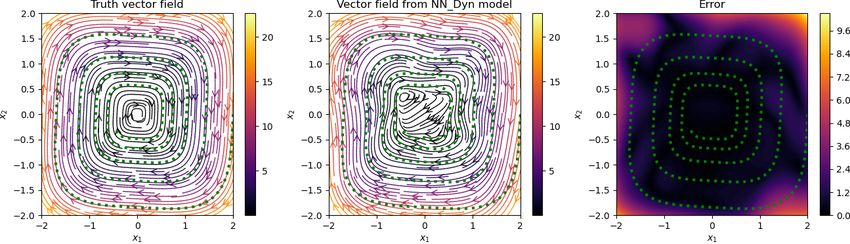
P. Goyal, P. Benner: Learning Dynamics from Noisy Measurements using DL                                        2

engineering studies such as process design, optimization, predictions, and control. Conventional approaches
based on physical laws, and empirical knowledge are often used to derive dynamical models. However, this
is impenetrable for many complex systems, e.g., understanding the Arctic ice pack dynamics, sea ice, power
grids, neuroscience, or finance, to only name a few applications.. Data-driven methods to discover models
have enormous potential to better understand transient behaviors in the latter cases. Furthermore, data
acquired using imaging devices or sensors are contaminated with measurement noise. Therefore, systematic
approaches that learn a dynamic model with proper treatment of noise are required. In this work, we discuss
a deep learning-based approach to learn a dynamic model by attenuating noise with a Runge-Kutta scheme,
thus allowing us to learn models quite accurately even when data are highly corrupted with measurement
noise.
   Data-driven methods to learn the governing equations of dynamic models have been studied for several
decades, see, e.g., [1–3]. Learning linear models from input-output data goes back to Ho and Kalman
[4]. There have been several algorithmic developments for linear systems, for example, the eigensystem
realization algorithm (ERA) [5, 6], and Kalman filter-based approaches [7–9]. Dynamic mode decomposition
(DMD) has also emerged as a promising approach to construct models from input-output data and has been
widely applied in fluid dynamics applications, see, e.g., [10–12]. Furthermore, there has been a series of
developments to learn nonlinear dynamic models. This includes, for example, equations free modeling [13],
nonlinear regression [14], dynamic modeling [15], and automated inference of dynamics [16–18]. Utilizing
symbolic regression and an evolutionary algorithm [19, 20], learning compact nonlinear models becomes
possible. Moreover, leveraging sparsity (also known as sparse regression), several approaches have been
proposed [21–26]. We also mention the work [27] that learns models using Gaussian process regression.
All these methods have particular approaches to handle noise in the data. For example, sparse regression
methods, e.g., [21,22,26] often utilize smoothing methods before identifying models, and the work [27] handles
measurement noise as data represented like a Gaussian process.
   Even though the aforementioned nonlinear modeling methods are appealing and powerful in providing
analytic expressions for models, they are often built upon model hypotheses. For example, the success of
sparse regression techniques relies on the fact that the nonlinear basis functions, describing the dynamics, lies
in a candidate features library. For many complex dynamics, such as the melting Arctic ice, the utilization
of these methods is not trivial. Thus, machine learning techniques, particularly deep learning-based ones,
have emerged as powerful methods capable of expressing any complex function in a black-box manner given
enough training data. Neural network-based approaches in the context of dynamical systems have been
discussed in [28–31] decades ago. A particular type of neural networks, namely recurrent neural networks,
intrinsically models sequences and is often used for forecasting [32–36]. Deep learning is also utilized to
identify a coordinate transformation so that the dynamics in the transformed coordinates are almost lin-
ear or sparse in a high-dimensional feature basis, see, e.g., [37–40]. Furthermore, we mention that classical
numerical schemes are incorporated with feed-forward neural networks to have discrete-time steppers for pre-
dictions, see [30, 41–43]. The approaches in [30, 41] can be interpreted as nonlinear autoregressive models [3].
A crucial feature of deep learning-based approaches that integrates numerical integration schemes is that
vector fields are estimated using neural networks. Also, time-stepping is done using a numerical integration
scheme. However, measurement data are often corrupted with noise, and these mentioned approaches do not
perform any specific noise treatment. The work in [44] proposes a framework that explicitly incorporates
the noise into a numerical time-stepping method. Though the approach has shown promising directions, its
scalability remains ambiguous as the approach explicitly needs noise estimates and aims to decompose the
signal explicitly into noise and ground truth.
   Our work introduces a framework to learn dynamics models by innovatively blending deep learning with
numerical integration methods from noisy and sparse measurements. Precisely, we aim at learning two
networks; one that implicitly represents given measurement data and the second one approximates the
vector field; we connect these two networks by enforcing a numerical integration scheme as depicted in
Figure 1.1. The appeal of the approach is that we do not require an explicit estimate of noise to learn a
model. Furthermore, the approach is applicable even if the dependent variables are sampled on different
time grids. The remaining structure of the paper is as follows. In Section 2, we present our deep learning-
based framework for learning dynamics from noisy measurements by combining two networks. One of these
networks implicitly represents measurement data, and the other one approximates the vector field. It is
followed by connecting these two networks by enforcing a numerical integration scheme. We briefly discuss

Preprint.                                                                                             2021-09-24
P. Goyal, P. Benner: Learning Dynamics from Noisy Measurements using DL 3
a Noisy data b Find implicit respresentation of data c x(ti )
noisy data
clean data
1.5 NφDyn
1.0
w(t)
0.5 hi
×
0.0 2
×
0.5 t hi
+
x(t)
Data 6
Runge-Kutta Constraint
2
1 NφDyn
0 50 0
100 150 200 1
)
v(t
Time 250 300 2
hi
×
(t) 350
×
400 3 2
hi
+
3
NφDyn
Implicit respresentation of denoised data hi
×
×
e hi
Noisy measurements
d
Denoised data
Loss :=
+
clean data 3
x(t) = NθI (t),
ky (t) − x(t)k NφDyn
2.0
1.5 and | data {z }
1.0 Implicit loss hi
d
w(t)
0.5
×
0.0 x(t) ≈ NφDyn(x(t)) + λRK x(ti+1) − NφDyn (x(ti)) 6
0.5 dt | {z }
+
1.0
3 RK mismatch loss
2 Denoised d ≈
0 50 0
1
+ λGrad x − NφDyn(x)
100 1 dt
)
150 200
v(t
Time 250 300
(t) 350
2 | {z } x(ti+1 )
400 Gradient loss
Figure 1.1: The figure illustrates the framework to de-noise temporal data and learns a model approximating
the vector field. For this, we aim at finding an implicit representation of measurement data by a network
(denoted by NθI ) and another network for the vector field (denoted by NφDyn ). These two networks are
connected by enforcing a Runge-Kutta scheme, shown in (c), on the output of the network NθI . Once the
loss is minimized, we obtain an implicit network for de-noised data and a model NφDyn , approximating the
vector field.
suitable architectures of neural networks for our framework in Section 4. In the subsequent section, we
demonstrate the effectiveness of the proposed methodology using various synthetic data with increasing
levels of noise, describing various physical phenomena. We conclude the paper with a summary and future
research directions.
2 Learning Dynamical Models using Deep Learning Constraint by a
Runge-Kutta Scheme
Data-driven methods to learn dynamic models have flourished significantly in the last couple of decades.
For these methods, quality of measurement data plays a significant role to ensure accuracy of the learned
models. While dealing with real-world measurements, sensor noise in the collected data is inevitable. Thus,
before employing any data-driven method, de-noising the data is a vital step and is typically done using
classical methods, e.g., smothering techniques, moving averages, or the noise is explicitly estimated along
with dynamics that imposes a challenge in a large-scale setting. In this section, we discuss our framework
to learn dynamic models using noisy measurements without explicitly estimating noise. To achieve the goal,
we utilize the powerful approximation capabilities of deep neural networks and its automatic differentiation
feature with a numerical integration scheme. In this work, we focus on the fourth-order Runge-Kutta (RK4)
scheme; however, the framework is flexible to use any other numerical integration scheme, or higher-order
Runge-Kutta schemes. Before we proceed further, we briefly outline the RK4 scheme. For this, let us consider
an autonomous nonlinear differential equation:
d
x(t) = g(x(t)), x(0) = x0 , (2.1)
dt
Preprint. 2021-09-24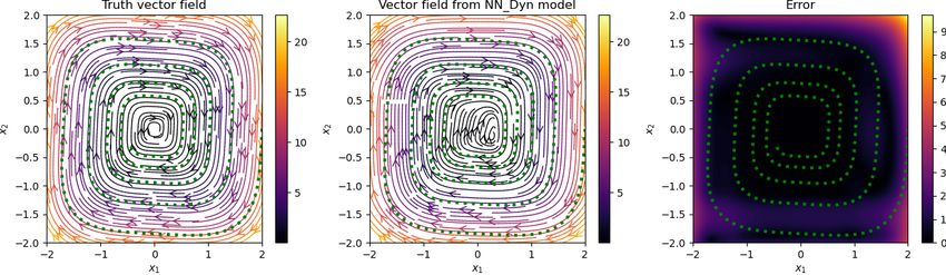
P. Goyal, P. Benner: Learning Dynamics from Noisy Measurements using DL                                                          4

where x(t) ∈ Rn denotes the solution at time t, and the continuous function g(·) : Rn → Rn defines the
vector field. Furthermore, the solution x(ti+1 ) can be explicitly given as follows:
                                                               Z    ti+1
                                        x(ti+1 ) = x(tj ) +                g(x(τ ))dτ .                                       (2.2)
                                                                   ti
                                                               |            {z      }
                                                                             Gi

Furthermore, we approximate the integral term Gi using the RK4 scheme, which can be determined by a
weighted sum of the vector field computed at specific locations as follows:

                                             1      1      1      1
                                   Gi ≈ hi     k1 + k2 + k3 + k4 ,                             (2.3)
                                             6      3      3      6

where hi = ti+1 − ti , and

                                           hi                              hi
        k1 = g (x(ti )) ,   k2 = g x(ti ) + k1 ,            k3 = g x(ti ) + k2 ,                 k4 = g (x(ti ) + hi k3 ) .
                                           2                               2

Consequently, we can write

                                                     1     1    1    1
                        x(ti+1 ) ≈ x(ti ) + hi         k1 + k2 + k3 + k4                 =: ΠRK (x(ti )) .                    (2.4)
                                                     6     3    3    6

In what follows, we assume that the ground-truth (or de-noised) sequence approximately follows the RK4 steps.
We emphasize that the information of the vector field at x is directly utilized in the RK4 scheme.
   Having described the RK4 scheme, we are now ready to proceed to discuss our framework to learn dynamical
models from noisy measurements by blending deep neural networks with the RK4 scheme. The approach
involves two networks. The first network implicitly represents the variable as shown in Figure 1.1(b), and
the second network approximates the vector field, or the function g(·). These two networks are connected
by attenuating the RK4 constraints. That is, the output of the implicit network is not only in the vicinity
of the measurement data but also approximately follows the RK4 scheme as depicted in Figure 1.1(c). To
make things mathematically precise, let us denote noisy measurement data at time ti by y(ti ). Furthermore,
we consider a feed-forward neural network, denoted by NθI parameterized by θ, that approximately yields an
implicit representation of measurement data, i.e.,

                                                 NθI (ti ) := x(ti ) ≈ y(ti ),                                                (2.5)

where i ∈ {1, . . . , M } with M being the total number of measurements. Additionally, let us denote another
neural network by NφDyn parameterized by φ that approximates the vector field g(·). We connect these two
networks by enforcing the output of the network NθI to respects the RK4 scheme, i.e.,

                                                                        d
                              x(ti+1 ) ≈ ΠRK x(ti ),        and            x(ti ) ≈ NφDyn (x(ti )) .                          (2.6)
                                                                        dt
As a result, our goal becomes to determine the network parameters {θ, φ} such that the following loss is
minimized:
                                   L = LMSE + λRK LRK + λGrad LGrad ,                              (2.7)
where
   • LMSE denotes the root mean square error of the output of the network NθI and noisy measurements,
     i.e.,
                                            M
                                         1 X                       2
                                                 NθI (ti ) − y(ti ) .                           (2.8)
                                        M i=1
      The loss enforces measurement data to be close to the output of the implicit network.

Preprint.                                                                                                              2021-09-24
P. Goyal, P. Benner: Learning Dynamics from Noisy Measurements using DL                                   5

   • The term LRK links the two networks by the RK4 scheme. Precisely, the term LRK castigates the
     mismatch between x(ti+1 ) and ΠRK x(ti ), i.e.,
                                           M −1
                                         1 X                             2
                                                kx(ti+1 ) − ΠRK (x(ti ))k ,                            (2.9)
                                         M i=1

      and the parameter λRK defines its weight in the total loss.
   • The vector field at the output of the implicit network can also be computed directly using automatic
     differentiation, but it also can be computed using the network NφDyn . The term LGrad penalizes its
     mismatch as follows:
                                            M
                                         1 X
                                                                       2
                                                                d
                                                NφDyn (x(ti )) − x(ti ) ,                           (2.10)
                                        M i=1                   dt

and λGrad is its corresponding regularization parameter.
   The total loss L can be minimized using a gradient-based optimizer such as Adam [45]. Once the networks
are trained and have found their parameters that minimize the loss, we can generate the de-noised variables
using the implicit network NθI , and the vector field by the network NφDyn . Note that due to the implicit
nature of the network, the measurement data can be at variable time steps, and we can estimate the solution
at any arbitrary time. Moreover, we also obtain the network NφDyn (·) that approximately provides the vector
field for x; hence, one can use it to make predictions.

3 Possible Extensions of the Approach
In many instances, dynamical processes may involve system parameters, and by varying them, the processes
exhibit different dynamics. Also, on several occasions, dynamics are governed by underlying partial dif-
ferential equations. In this section, we shortly discuss extensions of the proposed approach to these two
cases.

3.1 Parametric models
The approach discussed in the previous section readily extends to parametric cases. Let us consider a
parametric differential equation as follows:
                                          d
                                             x(t; µ) = g(x(t; µ), µ),                                  (3.1)
                                          dt
where µ ∈ Rd is the system parameter. To handle parameter µ, we can simply take the parameter µ as
an additional input to the implicit network NθI that yields the dependent variables at a given time and
parameter. Furthermore, to learn the function g(x(t; µ), µ), we take the parameter µ as an input as well
along with x(t; µ) to obtain a parameterized dynamical model to predict the vector field at a given x and
parameter.

3.2 Partial differential equations
Many cases, for example, dynamics of flows, dynamical behaviors, are governed by partial differential equa-
tions; thus, the dependent variable x is highly influenced by its neighbors. In such a case, we construct an
implicit representation for measurement data such that the implicit network takes time t and the spatial
coordinates ζ as inputs and yields dependent variable x(t, ζ). Then, we compute Xζ containing x at user-
specified spatial locations. This can be used to learn a dynamic model that describes dynamics at these
spatial locations. Consequently, with these discussed alterations, one can employ the approach discussed in
the previous section. The strength of the approach is that the collected measurement data can be at any
arbitrary spatial location. These locations can also vary with time since we construct an implicit network
that is independent of any structure in the collected measurements.

Preprint.                                                                                         2021-09-24
P. Goyal, P. Benner: Learning Dynamics from Noisy Measurements using DL 6
(a) Multi-layer perceptron (c) Residual network (convolutional)
Residual block
Residual block
Residual block
3 × 3conv, k
3 × 3conv, n
3 × 3conv, k
ELU
Output
Input
3 × 3conv, k
t x(t)
+
ELU
N ×M ×n N ×M ×k N ×M ×k N ×M ×k N ×M ×k N ×M ×n N ×M ×n
(b) Residual network (fully connected)
Residual block
Residual block
Residual block
Output
Input
Linear
Linear
Linear
Linear
ELU
ELU
+
n×1 k×1 k×1 k×1 k×1 k×1 n×1
Figure 4.1: The figure shows three potential simple architectures that can be used to learn either implicit
representation or to approximate the underlying vector field. Diagram (a) is a simple multi-layer perceptron,
and (b) is a residual-type network but fully connected, and (c) is a residual-type network with convolutional
layers. The notation {3 × 3 conv, k} means k filters of 3 × 3 receptive field.
4 Suitable Neural Networks Architectures
Here, we briefly discuss neural network architectures suitable for our proposed approach. We require two
neural networks for our framework, one for learning the implicit representation NθI and the second one NθDyn
is to learn the vector field. For implicit representation, we use a fully connected multi-layer perceptron (MLP)
as depicted in Figure 4.1(a) with periodic activation functions (e.g., sin) [46] which has shown its ability to
capture finely detailed features as well as the gradients of a function. To approximate the vector field, we
consider two possibilities depending on applications. If the data do not have any spatial dependency, then we
consider a simple residual-type network as illustrated in Figure 4.1(b) with exponential linear unit (ELU) as
an activation function [47]. We choose ELU as the activation function since it is continuous and differentiable
and resembles a widely used activation function, namely rectified linear unit (ReLU). On the other hand,
when the data has spatial correlations, e.g., dynamics in data are governed by a partial differential equation,
then it is more intuitive to use a convolutional neural network (CNN) with residual connections as depicted
in Figure 4.1(c). It explicitly makes use of the spatial correlation. For CNN, we also employ the batch
normalization scheme [48] after each convolution step for a better distribution of the input to the next layer
and use ELU as an activation function.
5 Numerical Experiments
In this section, we investigate the performance of the approach discussed in Section 2 to de-noise measurement
data as well as learning a model for estimating the vector field. To that aim, we consider data obtained by
solving several (partial) differential equations that are then corrupted using white Gaussian noise by varying
the noise level. For a given percentage of noise, we determine the noise as follows:
ν ∼ N (0, Σ) , with Σ = Noise%. (5.1)
We have implemented our framework using the deep learning library PyTorch [49] and have optimized all
networks together using the Adam optimizer [45]. Furthermore, to train implicit networks, we map the input
data to [−1, 1] as recommended in [46]. Additionally, to avoid over-fitting, we add L2 -regularization (also
Preprint. 2021-09-24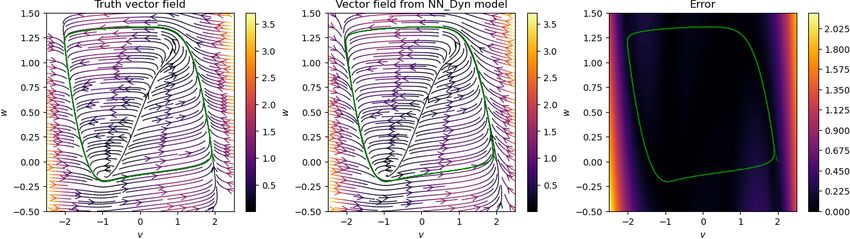
P. Goyal, P. Benner: Learning Dynamics from Noisy Measurements using DL 7
Layers or
Example Networks Neurons Learning rates
residual blocks
For implicit representation 20 4 5 · 10−4
FHN
For approximating vector field 20 4 10−3
For implicit representation 20 4 5 · 10−4
Cubic oscillator
For approximating vector field 20 4 10−3
Table 5.1: The table shows the information about network architectures and learning rates.
referred to as weight decay) of the parameters of the networks and set the regularization parameter to 10−4
for all examples. All the networks are trained for 15 000 epochs with batch size 1, and learning rates used to
train networks are stated in each example in their respective subsections. We have run all our experiments
on a Nvidia® A100 GPU.
5.1 Fitz-Hugh Nagumo model
In the first example, we discuss the Fitz-Hugh Nagumo (FHN) model that explains neural dynamics in a
simplistic way [50]. This has been used as a test case to discover the model using dictionary-based sparse
regression [26]. The dynamics are given as follows:
v(t) = v(t) − w(t) − 31 v(t)3 + 0.5,
(5.2)
w(t) = 0.040v(t) − 0.028w(t) + 0.032,
where v(t) and w(t) describe the dynamics of activation and de-activation of neurons. We collect 4 000
measurements in time t ∈ [0, 400] at a regular interval by simulating using the initial condition [v(0), w(0)] =
[2, 0]. We then corrupt the data artificially by adding various levels of noise. We build two networks with
the information provided in Table 5.1. We have set both the parameters λDyn and λGrad in the loss function
(2.7) to 1.
Having trained networks, we obtain de-noised measurement data using the implicit network and estimate
the vector field using the neural network. The results are shown in Figure 5.1. The figure demonstrates
the robustness of the approach with respect to noise. The method can recover the data very close to clean
data (see the first two columns of the figure) even when the measurements are corrupted with relatively
more significant noise, e.g., 20% to 40%. Furthermore, the vector field is estimated quite accurately, at least
in the regime of the collected measurements, see the third and fourth columns of the figure. However, as
expected, the vector field estimates are inadequate away from the measurements, thus, showing the limitation
in extrapolating to the regime where no data is available. Nevertheless, this can be improved by collecting
more measurements in a different regime by varying initial conditions.
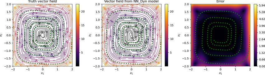
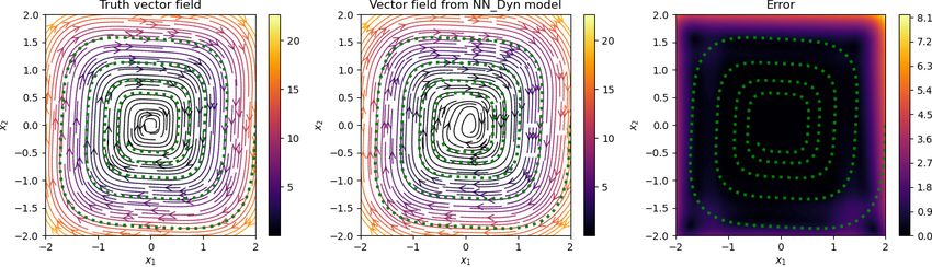
5.2 Cubic damped model
In the second example, we consider a damped cubic system, which is described by
ẋ(t) = −0.1x(t)3 + 2.0y(t)3 ,
(5.3)
ẏ(t) = −2.0x(t)3 − 0.1y(t)3 .
It has been one of the benchmark examples in discovering models using data, see, e.g., [26, 51] but there,
it is assumed that the dynamics can be given sparsely in a high-dimensional feature dictionary. Here, we
do not make any such assumptions and instead learn the vector field using a neural network along the line
of [52]. For this example, we take 2 500 data points in the time interval [0, 10] by simulating the model
using the initial condition [2, 0] as done in [52]. We add various levels of noise in the clean data to have
noisy measurements synthetically. We, again, perform similar experiments as done in the previous example.
We construct neural networks for implicit representation and the vector field with the parameters given in
Table 5.1.
Having trained networks with parameters λDyn = 1 and λGrad = 0.05 in the loss function (2.7), we have
an implicit network to obtain de-noised signal and a neural network approximating the vector field. We plot
Preprint. 2021-09-24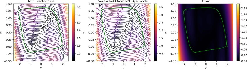
P. Goyal, P. Benner: Learning Dynamics from Noisy Measurements using DL                                         8

                                                                                                          Clean data
                                                                                                            Noise 5%
                                                                                                            Noise 10%
                                                                                                            Noise 20%
                                                                                                            Noise 40%

Figure 5.1: Fitz-Hugh Nagumo model. The figure shows the performance of the proposed approach to recover
the truth signal. In the first and second columns, we present the noisy, clean, and recovered data. In the
third and fourth columns, we show the estimate of the vector field using the learned neural model for it, and
the green dots are the clean data in the domain. We observe that the vector fields are very well estimated in
the regime of the collected data.

the results in Figure 5.2, where we show noisy, clean, and de-noised data in the first two columns, and in
the third and fourth columns, we plot the streamlines of the vector field, obtained using the trained neural

Preprint.                                                                                          2021-09-24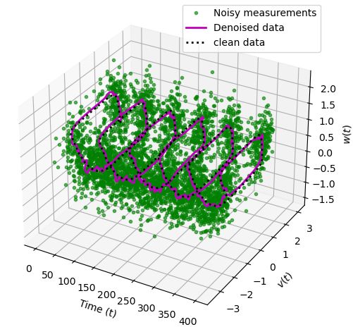
P. Goyal, P. Benner: Learning Dynamics from Noisy Measurements using DL                                             9

                                                                    Neurons         Layers or
            Example                       Networks                                                 Learning rates
                                                                    or filters   residual blocks
                               For implicit representation             10               4             5 · 10−4
      Burgers example
                              For approximating vector field            8               4               10−3
   Kuramoto–Sivashinsky        For implicit representation             50               4             5 · 10−4
        example               For approximating vector field           16               4               10−3

Table 5.2: The table shows the information about the network for Burgers and Kuramoto–Sivashinsky ex-
amples.

network. We observe that the de-noised data faithfully matches with the clean data even for a high noise
level, and the vector field is also close to the ground truth, at least in the region where measurement data
are sampled. However, in the region where no data are available, the vector field approximation is poor, as
one can expect. However, having richer data covering a larger training regime can improve the performance
of the neural network, approximating the vector field.

5.3 Burgers equation
Next, we examine the case, where collected measurements have spatial correlation as well, meaning there is
an underlying partial differential equation, describing the dynamics. Here, we consider a 1D viscous Burger
equation. It explains several phenomenons occurring in fluid dynamics and is governed by
                                   ∂u(t, ζ)
                                            = −µuζζ f (t, ζ) + u(t, ζ)uζ (t, ζ),                                 (5.4)
                                     ∂t
where µ is the viscosity; uζ and uζζ denote the first and second derivatives with respect to the spatial variable
ζ, and the equation is also subject to a boundary condition. We have taken the data from [53], followed
by artificially corrupting them using various levels of Gaussian white noise. In brief, the measurements are
collected at 256 grid point in the domain ζ ∈ [−8, 8] and at the time interval dt = 0.1. For more details, we
refer to [53].
   Since the data has spatial correlations, we make use of convolutional neural networks to learn the vector
field of u, instead of a classical MLP as shown in Figure 4.1. Thus, we build an MLP for the implicit
representation and a CNN with details given in Table 5.2. Once we train the network, in Figure 5.3, we plot
the performance of the proposed approach to de-noise the spatial-temporal data for an increasing level of
noise. We observe that the proposed methodology is able to recover the data faithfully even with significant
noise in data. Furthermore, in the last columns of Figure 5.3, we observe the approximating capability of the
                                             ∂
convolutional NN for the vector field, e.g., ∂t u(t, ζ). We observe that the model also predicts the vector field
with good accuracy. We mark that the vector field of the clean data is estimated using a finite-difference
scheme on the clean data since the true function is not known to us.

5.4 Kuramoto–Sivashinsky equation
In our last test case, we take the data of a chaotic dynamics which are obtained by simulating the Kuramoto–
Sivashinsky equation which is of form:
                              ∂
                                 u(t, ζ) = u(t, ζ)uζ (t, ζ) + uζζ (t, ζ) + uζζζζ (t, ζ),                         (5.5)
                              ∂t
where uζ , uζζ , and uζζζζ denote the first, second, and fourth derivatives with respect to ζ. The equation
explains several physical phenomena such as instabilities of dissipative trapped ion modes in plasma, or
fluctuation in fluid films, see, e.g., [54]. We again use the data provided in [53] for the equations which is
simulated using a spectral method with 1 024 spatial grid points and 251 time-steps. Since the dynamics
present in the data is very rich, complex, and exhibits chaotic behavior, we require networks that are more
expressive as compared to the previous example; the details about the networks are provided in Table 5.2.
   In Figure 5.4, we report the ability of our method to remove the noise from the spatial-temporal data.
We observe that the proposed methodology profoundly removes noise from the data. Also, the vector field

Preprint.                                                                                                2021-09-24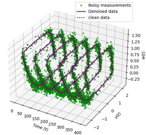
P. Goyal, P. Benner: Learning Dynamics from Noisy Measurements using DL                                   10

                                                                                                          Clean data
                                                                                                            Noise 5%
                                                                                                            Noise 10%
                                                                                                            Noise 20%
                                                                                                            Noise 40%

Figure 5.2: Damped cubic model. We visualize the noisy, clean, and de-noised signal for various levels of
noise in the measurement data (in the first two columns). We also show a comparison of the vector field
obtained using the neural network with the ground truth (in the last two columns). We observe that the
approach accurately recovers the clean data from the highly noisy measurements, and accurately predicts
the vector field for the model.

is approximated very well using the learned CNN (see the last column of the figure). The vector field of the
clean data is computed using a finite difference method. We draw particular attention to the last row of
Figure 5.4. The algorithm recovers several minor details that are damaged due to the presence of a high-level

Preprint.                                                                                          2021-09-24
P. Goyal, P. Benner: Learning Dynamics from Noisy Measurements using DL 11
clean data
1% noise
5% noise
10% noise
20% noise
Figure 5.3: Burgers’ equation: The figures show performance of the proposed framework to recover the
original spatio-temporal data for various levels of noise. The first and second columns are the noisy and de-
noised measurements, and the last column is the prediction of the vector field using the learning convolutional
neural network.
noise (20%).
Preprint. 2021-09-24P. Goyal, P. Benner: Learning Dynamics from Noisy Measurements using DL 12
clean data
1% noise
5% noise
10% noise
20% noise
Figure 5.4: Kuramoto–Sivashinsky equation: The figure shows the noisy measurements (the left column),
de-noised measurements (middle column), and the vector field approximation in the right column.
6 Discussion
In this work, we have presented a new paradigm for learning dynamical models from highly noisy (spatial)-
temporal measurement data. Our framework blends powerful approximation capabilities of deep neural
networks with a numerical integration scheme, namely the fourth-order Runge-Kutta scheme. The proposed
Preprint. 2021-09-24P. Goyal, P. Benner: Learning Dynamics from Noisy Measurements using DL 13
scheme involves two networks to learn an implicit representation of the measurement data and of the vector
field. These networks are combined by enforcing that the output of the implicit network respects the inte-
gration scheme. Furthermore, we highlight that the proposed approach can readily handle arbitrary sampled
points in space and time. In fact, the dependent variables need not be collected at the same time and the
exact location. This is because we first construct an implicit representation of the data that do not require
data to be of a particular structure.
We note that the approach becomes computationally expensive when the spatial dimension increases.
Indeed, it becomes impracticable when the data are collected for 2D or 3D space. A large system parameter
space imposes additional challenges. However, we know that the dynamics often lie in a low-dimensional
manifold. Therefore, in our future work, we aim to utilize the concept of low-dimensional embedding to
make learning computationally more efficient. Furthermore, we learn a dynamic model as a black-box neural
network. Hence, interpretability and generalizability remain opaque. In the future, it could be interesting
to combine or use the de-noised data with sparse or symbolic regression, as, e.g., in [53, 55, 56] to obtain an
analytic expression for a (partial) differential equations explaining the data.
References
[1] J.-N. Juang, Applied System Identification. Prentice-Hall, 1994.
[2] L. Ljung, System Identification – Theory for the User, 2nd ed. Upper Saddle River, NJ: Prentice-Hall,
1999.
[3] S. A. Billings, Nonlinear System Identification: NARMAX Methods in the Time, Frequency, and Spatio-
Temporal Domains. John Wiley & Sons, 2013.
[4] B. Ho and R. E. Kálmán, “Effective construction of linear state-variable models from input/output
functions,” Automatisierungstechnik, vol. 14, no. 1-12, pp. 545–548, 1966.
[5] J.-N. Juang and R. S. Pappa, “An eigensystem realization algorithm for modal parameter identification
and model reduction,” J. Guidance, Control, and Dyn., vol. 8, no. 5, pp. 620–627, 1985.
[6] R. W. Longman and J.-N. Juang, “Recursive form of the eigensystem realization algorithm for system
identification,” J. Guidance, Control, and Dyn., vol. 12, no. 5, pp. 647–652, 1989.
[7] J.-N. Juang, M. Phan, L. G. Horta, and R. W. Longman, “Identification of observer/Kalman filter
Markov parameters-theory and experiments,” J. Guidance, Control, and Dyn., vol. 16, no. 2, pp. 320–
329, 1993.
[8] M. Phan, L. G. Horta, J.-N. Juang, and R. W. Longman, “Linear system identification via an asymp-
totically stable observer,” J. Opt. Th. Appl., vol. 79, no. 1, pp. 59–86, 1993.
[9] M. Phan, J.-N. Juang, and R. W. Longman, “Identification of linear multivariable systems by identifi-
cation of observers with assigned real eigenvalues,” J. Astronautical Sci., vol. 40, no. 2, 1992.
[10] R. E. Kalman, “A new approach to linear filtering and prediction problems,” J. Fluid Engrg., vol. 82,
no. 1, 1960.
[11] P. J. Schmid, “Dynamic mode decomposition of numerical and experimental data,” J. Fluid Mech., vol.
656, pp. 5–28, 2010.
[12] J. H. Tu, C. W. Rowley, D. M. Luchtenburg, S. L. Brunton, and J. N. Kutz, “On dynamic mode
decomposition: Theory and applications,” J. Comput. Dyn., vol. 1, no. 2, pp. 391–421, 2014.
[13] I. G. Kevrekidis, C. W. Gear, J. M. Hyman, P. G. Kevrekidis, O. Runborg, C. Theodoropoulos et al.,
“Equation-free, coarse-grained multiscale computation: Enabling mocroscopic simulators to perform
system-level analysis,” Comm. Math. Sci., vol. 1, no. 4, pp. 715–762, 2003.
[14] H. U. Voss, P. Kolodner, M. Abel, and J. Kurths, “Amplitude equations from spatiotemporal binary-fluid
convection data,” Physical Rev. Lett., vol. 83, no. 17, p. 3422, 1999.
Preprint. 2021-09-24P. Goyal, P. Benner: Learning Dynamics from Noisy Measurements using DL 14
[15] H. Ye, R. J. Beamish, S. M. Glaser, S. C. Grant, C.-H. Hsieh, L. J. Richards, J. T. Schnute, and
G. Sugihara, “Equation-free mechanistic ecosystem forecasting using empirical dynamic modeling,” Proc.
Nat. Acad. Sci. U.S.A., vol. 112, no. 13, pp. E1569–E1576, 2015.
[16] M. D. Schmidt, R. R. Vallabhajosyula, J. W. Jenkins, J. E. Hood, A. S. Soni, J. P. Wikswo, and
H. Lipson, “Automated refinement and inference of analytical models for metabolic networks,” Phy.
Biology, vol. 8, no. 5, p. 055011, 2011.
[17] B. C. Daniels and I. Nemenman, “Automated adaptive inference of phenomenological dynamical mod-
els,” Nature Comm., vol. 6, no. 1, pp. 1–8, 2015.
[18] ——, “Efficient inference of parsimonious phenomenological models of cellular dynamics using S-systems
and alternating regression,” PLoS One, vol. 10, no. 3, p. e0119821, 2015.
[19] J. Bongard and H. Lipson, “Automated reverse engineering of nonlinear dynamical systems,” Proc. Nat.
Acad. Sci. U.S.A., vol. 104, no. 24, pp. 9943–9948, 2007.
[20] M. Schmidt and H. Lipson, “Distilling free-form natural laws from experimental data,” Science, vol.
324, no. 5923, pp. 81–85, 2009.
[21] S. L. Brunton, J. L. Proctor, and J. N. Kutz, “Sparse identification of nonlinear dynamics with control
(SINDYc),” IFAC-PapersOnLine, vol. 49, no. 18, pp. 710–715, 2016.
[22] N. M. Mangan, S. L. Brunton, J. L. Proctor, and J. N. Kutz, “Inferring biological networks by sparse
identification of nonlinear dynamics,” IEEE Trans. Molecular, Biological and Multi-Scale Comm., vol. 2,
no. 1, pp. 52–63, 2016.
[23] G. Tran and R. Ward, “Exact recovery of chaotic systems from highly corrupted data,” Multiscale
Modeling & Simulation, vol. 15, no. 3, pp. 1108–1129, 2017.
[24] H. Schaeffer, G. Tran, R. Ward, and L. Zhang, “Extracting structured dynamical systems using sparse
optimization with very few samples,” Multiscale Modeling & Simulation, vol. 18, no. 4, pp. 1435–1461,
2020.
[25] N. M. Mangan, J. N. Kutz, S. L. Brunton, and J. L. Proctor, “Model selection for dynamical systems via
sparse regression and information criteria,” Proceedings of the Royal Society A: Mathematical, Physical
and Engineering Sciences, vol. 473, no. 2204, p. 20170009, 2017.
[26] P. Goyal and P. Benner, “Discovery of nonlinear dynamical systems using a Runge-Kutta inspired
dictionary-based sparse regression approach,” arXiv preprint arXiv:2105.04869, 2021.
[27] M. Raissi and G. E. Karniadakis, “Hidden physics models: Machine learning of nonlinear partial differ-
ential equations,” J. Comput. Phys., vol. 357, pp. 125–141, 2018.
[28] S. Chen, S. A. Billings, and P. Grant, “Non-linear system identification using neural networks,” Intern.
J. Control, vol. 51, no. 6, pp. 1191–1214, 1990.
[29] R. Rico-Martinez and I. G. Kevrekidis, “Continuous time modeling of nonlinear systems: A neural
network-based approach,” in IEEE Int. Conf. on Neural Networks, 1993, pp. 1522–1525.
[30] R. Gonzalez-Garcia, R. Rico-Martinez, and I. Kevrekidis, “Identification of distributed parameter sys-
tems: A neural net based approach,” Computers & Chemical Engrg., vol. 22, pp. S965–S968, 1998.
[31] M. Milano and P. Koumoutsakos, “Neural network modeling for near wall turbulent flow,” J. Comput.
Phys., vol. 182, no. 1, pp. 1–26, 2002.
[32] Z. Lu, B. R. Hunt, and E. Ott, “Attractor reconstruction by machine learning,” Chaos: An Interdisci-
plinary Journal of Nonlinear Science, vol. 28, no. 6, p. 061104, 2018.
[33] S. Pan and K. Duraisamy, “Long-time predictive modeling of nonlinear dynamical systems using neural
networks,” Complexity, vol. 2018, 2018.
Preprint. 2021-09-24P. Goyal, P. Benner: Learning Dynamics from Noisy Measurements using DL 15
[34] J. Pathak, Z. Lu, B. R. Hunt, M. Girvan, and E. Ott, “Using machine learning to replicate chaotic
attractors and calculate Lyapunov exponents from data,” Chaos: An Interdisciplinary J. Nonlinear
Sci., vol. 27, no. 12, p. 121102, 2017.
[35] J. Pathak, A. Wikner, R. Fussell, S. Chandra, B. R. Hunt, M. Girvan, and E. Ott, “Hybrid forecasting
of chaotic processes: Using machine learning in conjunction with a knowledge-based model,” Chaos: An
Interdisciplinary J. Nonlinear Sci., vol. 28, no. 4, p. 041101, 2018.
[36] P. R. Vlachas, W. Byeon, Z. Y. Wan, T. P. Sapsis, and P. Koumoutsakos, “Data-driven forecasting of
high-dimensional chaotic systems with long short-term memory networks,” Proc. the Royal Society A:
Mathematical, Physical and Engineering Sciences, vol. 474, no. 2213, p. 20170844, 2018.
[37] B. Lusch, J. N. Kutz, and S. L. Brunton, “Deep learning for universal linear embeddings of nonlinear
dynamics,” Nature Comm., vol. 9, no. 1, pp. 1–10, 2018.
[38] N. Takeishi, Y. Kawahara, and T. Yairi, “Learning Koopman invariant subspaces for dynamic mode
decomposition,” in Proc. 31st Internat. Conf. Neural Information Processing Sys., 2017, pp. 1130–1140.
[39] E. Yeung, S. Kundu, and N. Hodas, “Learning deep neural network representations for Koopman op-
erators of nonlinear dynamical systems,” in American Control Conference (ACC). IEEE, 2019, pp.
4832–4839.
[40] K. Champion, B. Lusch, J. N. Kutz, and S. L. Brunton, “Data-driven discovery of coordinates and
governing equations,” Proc. Nat. Acad. Sci. U.S.A., vol. 116, no. 45, pp. 22 445–22 451, 2019.
[41] M. Raissi, P. Perdikaris, and G. E. Karniadakis, “Multistep neural networks for data-driven discovery
of nonlinear dynamical systems,” arXiv preprint arXiv:1801.01236, 2018.
[42] ——, “Physics-informed neural networks: A deep learning framework for solving forward and inverse
problems involving nonlinear partial differential equations,” J. Comput. Phys., vol. 378, pp. 686–707,
2019.
[43] M. Raissi, A. Yazdani, and G. E. Karniadakis, “Hidden fluid mechanics: Learning velocity and pressure
fields from flow visualizations,” Science, vol. 367, no. 6481, pp. 1026–1030, 2020.
[44] S. H. Rudy, J. N. Kutz, and S. L. Brunton, “Deep learning of dynamics and signal-noise decomposition
with time-stepping constraints,” J. Comput. Phys., vol. 396, pp. 483–506, 2019.
[45] D. P. Kingma and J. Ba, “Adam: A method for stochastic optimization,” arXiv preprint
arXiv:1412.6980, 2014.
[46] V. Sitzmann, J. Martel, A. Bergman, D. Lindell, and G. Wetzstein, “Implicit neural representations
with periodic activation functions,” in Adv. in Neural Information Processing Systems, vol. 33, 2020.
[47] D.-A. Clevert, T. Unterthiner, and S. Hochreiter, “Fast and accurate deep network learning by expo-
nential linear units (ELUs),” arXiv preprint arXiv:1511.07289, 2015.
[48] S. Ioffe and C. Szegedy, “Batch normalization: Accelerating deep network training by reducing internal
covariate shift,” in Internat. Conf. Machine Learning. PMLR, 2015, pp. 448–456.
[49] A. Paszke, S. Gross, F. Massa, A. Lerer, J. Bradbury, G. Chanan, T. Killeen, Z. Lin, N. Gimelshein,
L. Antiga et al., “Pytorch: An imperative style, high-performance deep learning library,” arXiv preprint
arXiv:1912.01703, 2019.
[50] R. FitzHugh, “Mathematical models of threshold phenomena in the nerve membrane,” The Bulletin
Math. Biophys., vol. 17, no. 4, pp. 257–278, 1955.
[51] S. L. Brunton, J. L. Proctor, and J. N. Kutz, “Discovering governing equations from data by sparse
identification of nonlinear dynamical systems,” Proc. Nat. Acad. Sci. U.S.A., vol. 113, no. 15, pp. 3932–
3937, 2016.
Preprint. 2021-09-24P. Goyal, P. Benner: Learning Dynamics from Noisy Measurements using DL 16
[52] S. Rudy, A. Alla, S. L. Brunton, and J. N. Kutz, “Data-driven identification of parametric partial
differential equations,” SIAM J. Appl. Dyn. Syst., vol. 18, no. 2, pp. 643–660, 2019.
[53] S. H. Rudy, S. L. Brunton, J. L. Proctor, and J. N. Kutz, “Data-driven discovery of partial differential
equations,” Sci. Adv., vol. 3, no. 4, p. e1602614, 2017.
[54] Y. Kuramoto, “Diffusion-induced chaos in reaction systems,” Progress of Theoretical Physics Supple-
ment, vol. 64, pp. 346–367, 1978.
[55] M. Cranmer, A. Sanchez-Gonzalez, P. Battaglia, R. Xu, K. Cranmer, D. Spergel, and S. Ho, “Discovering
symbolic models from deep learning with inductive biases,” in Adv. in Neural Information Processing
Systems, 2020.
[56] G.-J. Both, S. Choudhury, P. Sens, and R. Kusters, “DeepMoD: Deep learning for model discovery in
noisy data,” J. Comput. Phys., vol. 428, p. 109985, 2021.
Preprint. 2021-09-24You can also read