Data Extraction from Charts via Single Deep Neural Network - arXiv.org
←
→
Page content transcription
If your browser does not render page correctly, please read the page content below
Data Extraction from Charts via Single Deep Neural Network

                                                                             Xiaoyi Liu 1 Diego Klabjan 1 Patrick N Bless 2

                                                                 Abstract                                charts (Savva et al., 2011; Huang & Tan, 2007) based on
                                                                                                         traditional computer vision methods, which rely on compli-
                                             Automatic data extraction from charts is challeng-
                                                                                                         cated human-defined rules and thus are not robust. With the
                                             ing for two reasons: there exist many relations
                                                                                                         proliferation of deep learning, it is conceivable that the accu-
arXiv:1906.11906v1 [cs.CV] 6 Jun 2019

                                             among objects in a chart, which is not a common
                                                                                                         racy of chart component detection can be improved without
                                             consideration in general computer vision prob-
                                                                                                         complicated rules, i.e., by using raw images as input with no
                                             lems; and different types of charts may not be
                                                                                                         feature engineering or employment of other rules. Despite
                                             processed by the same model. To address these
                                                                                                         of this belief there is still lack of a single deep learning
                                             problems, we propose a framework of a single
                                                                                                         model for data extraction from charts.
                                             deep neural network, which consists of object
                                             detection, text recognition and object matching             We introduce a deep learning solution that automatically ex-
                                             modules. The framework handles both bar and                 tracts data from bar and pie charts and essentially converts a
                                             pie charts, and it may also be extended to other            chart to a relational data table. The approach first detects the
                                             types of charts by slight revisions and by aug-             type of a chart (bar or pie), and then employs a single deep
                                             menting the training data. Our model performs               learning model that extracts all of the relevant components
                                             successfully on 79.4% of test simulated bar charts          and data. There is one single model for bar charts and a
                                             and 88.0% of test simulated pie charts, while for           different one for pie charts. The entire framework has three
                                             charts outside of the training domain it degrades           stages: 1. chart type identification, 2. element detection,
                                             for 57.5% and 62.3%, respectively.                          text recognition, and bounding box matching through which
                                                                                                         the actual numerical data is extracted, and 3. inference. The
                                                                                                         first phase is a standard image classification problem. The
                                        1. Introduction                                                  most interesting part is the second phase where we rely on
                                                                                                         the Faster-RCNN model (Ren & Sun, 2015). We add several
                                        “Data everywhere information nowhere” is a common say-           components to the feature maps of regional proposals, e.g.,
                                        ing in the business world. Consider all of the presentations     text detection and recognition. The most significant part
                                        and reports lingering in folders of a company. They are          is the addition of relation network components that match,
                                        embellished with eye-appealing charts as images forming          e.g., part of the legend with a matching bar, a bar with the
                                        formidable data, but getting information from these charts       y-axis value, a slice in the pie chart with part of the legend.
                                        is challenging. To this end, a system that automatically         In order to make extraction from pie charts work, additional
                                        extracts information from charts would provide great bene-       novel tricks are needed; e.g., the model detects the angle
                                        fits in knowledge management within the company. Such            of each slice by attaching an RNN to regional proposals
                                        knowledge can be combined with other data sets to further        (since slices form a sequence when traversed in a clockwise
                                        enhance business value. We address this problem by devel-        manner), multiplies the feature map matrix of the regional
                                        oping a deep learning model that takes an image of a chart       proposal of the entire pie with an angle-dependent rotation
                                        as input and it extracts information in the form of categories   matrix, and then uses this rotated matrix in the relation net-
                                        being displayed, the relevant text such as the legend, axis      work. The last inference phase is using heuristics to produce
                                        labels, and numeric values behind the data displayed.            the final objects and data.
                                        There are existing tools for information extraction from         The model is trained on simulated charts based on Microsoft
                                              1                                                          Excel and the Matplotlib library. It is then evaluated on
                                                Department of Industrial Engineering and Manage-
                                        ment Science, Northwestern University, Evanston, USA             simulated test data, the Microsoft FigureQA charts data set
                                        2
                                          Intel Corporation, Chandler, USA. Correspondence to:           (Kahou & Bengio, 2017), and manually inspected charts
                                        Xiaoyi Liu , Diego             from Google Images. The results on the simulated test set
                                        Klabjan , Patrick N Bless            show our model performs successfully on 79.4% simulated
                                        .                                     bar charts and 88.0% on simulated pie charts. On charts
                                                                                                         from FigureQA and Google Images the performance drops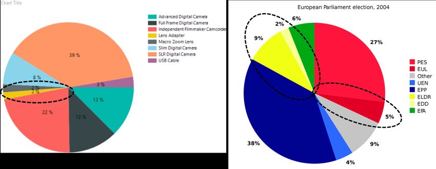
Data Extraction from Charts via Single Deep Neural Network

                                                                  Histograms of Oriented Gradients and the Scale Invariant
                                                                  Feature Transform descriptors for feature extraction and
                                                                  Support Vector Machine (SVM) for classification. Savva et
                                                                  al. (2011) have built a system called Revision to redesign
                                                                  charts, which includes chart classification, data extraction
                                                                  and visualization. Low-level image features are extracted
                                                                  for chart classification by SVMs.
                                                                  In recent years, deep learning techniques have made great
                                                                  progress in general image classification (Krizhevsky et al.,
                                                                  2012; Simonyan & Zisserman, 2012; He & Sun, 2016),
                                                                  which can be applied to chart classification. Among these
                                                                  methods, convolutional neural networks based methods are
   (a) Bar chart extraction        (b) Pie chart extraction       the most widely used, and Siegel et al. (2016) have trained
                                                                  both AlexNet (Krizhevsky et al., 2012) and ResNet-50 (He
        Figure 1. Framework for charts data extraction
                                                                  & Sun, 2016) on their annotated datasets including 60,000
                                                                  charts and 7 categories. VGG16 (Simonyan & Zisserman,
to 57.5% and 62.3% for bar and pie charts, respectively.          2012) is employed in our system.

Our main contributions are as follows.                            A chart includes a set of structural texts and data. In bar
                                                                  charts, texts can be categorized as title, axis-title, axis-tick
  • We propose a single deep learning model that extracts         or legend, and data information is encoded into the height
    information from bar charts. The new ideas of the             or width of bars. To extract the textual and graphical infor-
    model are the combination of text recognition, text           mation from bar charts, one must firstly detect the bounding
    detection, and pairwise matching of components within         boxes of texts and bars. Object detection is a common
    a single model. In particular, we design a new approach       problem in computer vision. With the development of deep
    for matching candidate components, e.g, an actual bar         learning techniques, there are two main kinds of methods:
    bounding box with an entry in the legend.                     1. RCNN (Girshick & Malik, 2014) includes two stages of
                                                                  generating region proposals and subsequent classification; 2.
  • We also propose another single deep learning model for        derivations fast-RCNN (Girshick, 2015) and Faster-RCNN
    pie charts. This model introduces an RNN component            (Ren & Sun, 2015) of RCNN, YOLO (Redmon & Farhadi,
    to detect angles in a pie chart, and a different strategy     2016) and SSD (Liu & Berg, 2016) use only one stage
    for matching non-rectangular patches.                         including both region proposing and classification, which
                                                                  usually perform better on training speed but worse on accu-
  • We use a pipeline where we first identify a chart type        racy of bounding box prediction (Huang & Murphy, 2017).
    by standard CNN-based classification. Once the chart          It is worth pointing out that Faster-RCNN produces higher
    type is identified, we employ one of the aforementioned       accuracy than YOLO and SSD at the expense of a higher
    models to extract information.                                training time. There are also some specially designed mod-
                                                                  els (Tian & Qiao, 2016; Shi & Belongie, 2017) which only
In Section 2, related work and methods for charts data extrac-    focus on text detection. Tian et al. (2016) use an anchor box
tion are reviewed. We show all components of our model            method to predict text bounding boxes. Shi et al. (2017)
and inference methods in Section 3. The computational             introduce a segment linking method that can handle oriented
results are discussed in Section 4.                               text detection.
                                                                  In terms of chart component detection, there are many works
2. Literature Review                                              done with traditional computer vision techniques. Zhou et
Automated chart analysis has been studied for many years,         al. (2000) combined Hough transform and boundary tracing
and the process of extracting data from charts in documents       to detect bars. Huang et al. (2007) have employed rules to
can be divided into four steps: chart localization and extrac-    detect chart components using edge maps. In (Savva et al.,
tion, chart classification, text and element detection, data      2011), bars or pies are detected by their shapes and color
reconstruction. Our work focuses on the last three steps.         information in pixels. By using deep learning techniques, all
                                                                  the texts and chart components can be detected in a model
Chart classification is a specific kind of image classification   automatically. There are already some works based on deep
problems. In 2007, Prasad et al. (2007) have presented            learning techniques; Cliche et al. (2017) have trained three
a traditional computer vision-based approach to classify          separate object detection models ReInspect (Stewart & Ng,
charts in five categories. This approach is based on the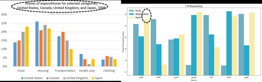
Data Extraction from Charts via Single Deep Neural Network
2016) to detect tick marks, tick labels and points in different 3.1. Background
resolutions, which are finally combined to extract data from
3.1.1. FASTER -RCNN
a scatterplot. Poco et al. (2017) have employed a CNN to
classify each pixel as text or not in a chart and then remove Faster RCNN uses a single convolutional neural network to
all non-text pixels. create feature maps for each predefined regional proposal
Data reconstruction is followed after chart component de- called also anchor proposal and predicts both a class label
tection. Data reconstruction also can be divided into text and bounding box for each anchor proposal. The first part
recognition and numerical data extraction. All detected text in Faster-RCNN is the Region Proposal Network (RPN),
bounding boxes are processed by a text recognition model. which yields a feature map for each anchor proposal. During
Tick labels are combined with the coordinate positions to the second part, two branches predict a class and a more
predict the coordinate-value relation. Other graphical com- accurate bounding box location for each anchor proposal.
ponents are processed by these coordinate-value relations, In the model, CNN is used to generate a single feature map.
which give all the data corresponding to an input chart. Anchor proposals are then selected as follows. A predefined
There is another challenging problem during this process: grid of pixels are used as centers of proposals. Each center
matching objects between different categories, which has pixel is associated with a fixed number of bounding boxes of
been studied by a few researchers. In (Siegel & Farhadi, different sizes centered at the pixel. These anchor proposals
2016), the matching task is formulated as an optimal-path- are identified with the viewing field in the original image
finding problem with features combined from CNN and to identify the ground truth of the class and the precise
pixels. Samira et al. (2017) have trained a model with a bounding box location.
baseline of Relation Networks (RN) (Santoro & Lillicrap,
2017) to build the relationship between objects and answer 3.1.2. R ELATION N ETWORKS
questions related with it. RNs (Santoro & Lillicrap, 2017) were proposed by Santoro
In our work, a single deep neural net is built to predict all et al. to solve the relation reasoning problem by a simple
objects’ bounding boxes and classes, to recognize texts of neural network module, which is appended after a series
textual objects, and match objects in an chart image, which of convolutional neural layers. An RN firstly concatenates
is very different from all aforementioned works because the object features from the last convolutional layer of two
each prior work on bar and pie charts addresses only a single objects and then employs a fully connected layer to predict
aspect leading to brittle solutions. We also introduce brand their true/false relation. The loss function component reads
new concepts and approaches such as rotations and angles
in conjunction with recurrent neural nets, and supervised
angle learning.
1 X
3. Model RN (O) = fφ 2 gθ (oi , oj ) (1)
N i,j
Our model uses Faster-RCNN (Ren & Sun, 2015) as the
object detection part to detect all the elements in a chart,
and then uses the idea from RNs (Santoro & Lillicrap, 2017)
as the object-matching part to match elements between dif- where O ∈ RN ×C is the matrix in which the i0 th row
ferent classes. We use Faster-RCNN over YOLO or SSD contains object representation oi . Here, gθ calculates the
because of higher accuracy. The price is higher training time. relation between a pair of objects and fφ aggregates these
CRNN (Shi & Yao, 2017) is employed as the text recog- relations and computes the final output of the model.
nition part in our model. All these parts are summarized
next. 3.1.3. CRNN
We build our model on Faster-RCNN because an accurate CRNN (Shi & Yao, 2017) is a text recognition model, which
prediction of bounding box locations is more important in is based on the popular CNN-RNN pipeline for text recog-
chart component detection compared with general object nition. It has gained state-of-art accuracy on several text
detection problems. recognition challenges. This model contains 7 convolutional
layers for feature extraction followed by 2 bidirectional
LSTM layers for sequence labeling and a transcription layer
on top of them. A sequence is a sequence of characters and
the input to an LSTM cell is a fixed width window in the
feature map (which keeps sliding from left to right to form
a sequence).
Data Extraction from Charts via Single Deep Neural Network

3.2. Main Model                                                    an IoU overlap to ground truth higher than a threshold are
                                                                   saved and sorted by their confidence. The top 256 of them
The first step in data extraction is to determine the chart
                                                                   are then fed into the regression neural network.
types (bar or pie) which consequently involves the corre-
sponding model for each type. The classification model is
                                                                   3.2.2. O RIENTED T EXT R ECOGNITION
built based on VGG16.
                                                                   The original Faster-RCNN model generates only horizontal
Faster-RCNN is employed as the backbone of our model,
                                                                   bounding boxes, which may contain texts with orientation.
with its two outputs, a class label, and a bounding box
                                                                   Besides the regression layer for localization, a new regres-
offset, for each candidate object augmented by additional
                                                                   sion layer for orientation is added under the branch for text
components. In our bar chart data extraction model, two
                                                                   recognition, see Figure 1 .
additional branches are added: a text recognition branch is
added after proposals with a predicted label of text, and an       Our text recognition branch is added after the Faster-RCNN
object-matching branch is added for all possible proposal          model and takes all proposals predicted as text by the classi-
combinations. Another angle prediction branch is added in          fication layer in Faster-RCNN. The text recognition branch
the pie chart data extraction model, and the object-matching       detects the orientation of the text in each text bounding box
branch is revised to capture slices. In bar charts, the RN         firstly and then rotates the feature map by the detected ori-
components try to match bars with a legend component or            entation using an affine transformation, which is similar to
x-axis label, and the height of a bar with a y-axis value. In      the Spatial Transformer Network (Jaderberg & Zisserman,
pie charts, we attempt to match each slice with a legend           2015), except that we use the orientation angle for super-
component.                                                         vised learning. In summary, the loss function includes the
                                                                   L2 loss Lorientation of the angle (the ground truth for angle
In order to handle non-horizontal text such as y-axis labels, a
                                                                   in training is known).
regression layer to predict orientation is added as part of the
text recognition branch. The feature map is then rotated by        We apply two-layer bidirectional LSTM to predict the se-
the angle and then CRNN is applied. The object-matching            quence labels of characters, followed by a sequence-to-
branch is inspired by the idea of RN by concatenating two          sequence mapping to words. The conditional probabilities
object features if class predictions are high for the classified   defined in CTC (Graves & Schmidhuber, 2006) are adopted
two objects. Figure 1 depicts the model.                           as the loss function of the recognition model.
We next provide details of these components. The first three       The loss function of the branch for oriented text recognition
sections apply to both bar and pie chart data extraction,          is
while the last section explains the enhancements made in                      Ltext = λo Lorientation + λC LCT C             (2)
pie chart data extraction.
                                                                   3.2.3. O BJECT M ATCHING
3.2.1. O BJECT D ETECTION
                                                                   There is an object matching branch appended after the fea-
Our object detection method is based on Faster-RCNN,               ture map (Conv5 3) generated by Faster-RCNN, which aims
which adopts VGG16 (Simonyan & Zisserman, 2012) as                 to match image patches from different categories.
the backbone. The top layer of the convolutional feature
                                                                   Our object matching branch is similar to RN but without
map (Conv5 3) is used to generate a manageable number
                                                                   the summation of feature maps, and the output of RN is
of anchor bounding boxes of all chart components. Con-
                                                                   normalized to better predict whether the input object pair is
sidering that the texts and bars have substantial variety in
                                                                   related or not
height/width ratios and can be of arbitrary orientation, and
the tick marks are always small, the aspect ratios of anchor                  OM (oi , oj ) = fφ (g(oi , oj )) ∈ [0, 1]        (3)
boxes are set to (0.1, 0.2, 0.5, 1.0, 2.0, 5.0, 10.0), while the
scales are set to (2, 4, 8, 16, 32). Scale of 4 refers to 4 × 4    where g is the concatenation operation and fφ refers to a
pixels in the feature map.                                         fully connected neural network. Here o is the feature map
There is no resizing of the input images because a resizing        of an anchor proposal.
procedure would lose the resolution for text in the image.         The loss function of the object matching branch between
Some texts are already very small in the original image            types U, V is formulated as
and cannot be distinguished even by humans after resizing.                      X
The flexible size of the input image affects the size of the        LOM =             H(Poi ) · H(Poj )
resulting convolutional feature maps. For example, a feature                 oi ∈U,oj ∈V
map of size m×n generates m×n×35 candidate bounding                                        · KL(yoi ,oj ||sof tmax(OM (oi , oj )))
boxes through the anchor mechanism. Only candidates with                                                                        (4)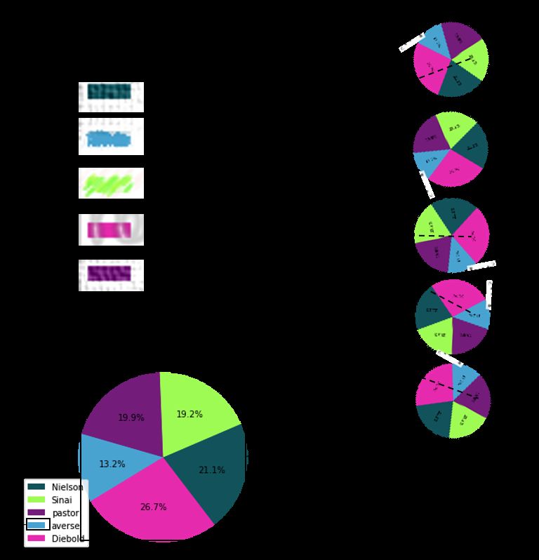
Data Extraction from Charts via Single Deep Neural Network

where yoi ,oj is the ground truth, KL is Kullback–Leibler        and legends for the non-rectangular shapes of slices.
divergence and H is a smooth approximation to the indicator
                                                                 In the pie chart object-matching model, the feature map for
function
                                  1                              each slice is generated from rotating the feature map of the
                H(x) =                                  (5)      whole pie by the angle of its boundary, so that the rotated
                         1 + exp( −k(x−τ
                                    1−τ
                                         )
                                           )
                                                                 feature map can have its corresponding slice in a specific
where τ is a threshold parameter and k is another parameter      region. The rotation is done by an affine transformation. We
controlling the steepness of the function near τ . Types         define the horizontal ray from left to right as zero degree
{U, V } in bar chart data extraction are {bar, legend sample}    and counter-clockwise as the positive direction, so all of
and in pie chart data extraction are {pie, legend}. We also      the feature maps have their corresponding slice features on
use the same model to match textual objects with other           the right-center region in the whole feature maps. Figure 3
objects while oi in above equations refers to the position       illustrates the strategy.
of each object. These types of {U, V } cover {y-tick label,      The object matching part is similar to the one for bar charts,
y-tick mark} and {legend sample, legend label}. We found         which concatenates the feature map of each legend and each
that this works much better than feature map vectors.            rotated feature map of the pie and predicts their relationship.
                                                                 This component learns which region of the feature map is
3.2.4. P IE C HART-BASED E NHANCEMENTS                           in focus.
Data extraction for pie charts is more challenging than for
bar charts since a slice is hard to detect using a rectangular
bounding box. Instead of generating each proposal bound-
ing box for each slice, we only predict the location of the
whole pie and the angle of each slice’s boundary based on
the feature map of the pie. Obtaining all the boundary angles
gives the information of the proportion of the pie chart.

                                                                            Figure 3. Pie chart object-matching model

   Figure 2. Angle prediction branch for pie chart extraction    3.2.5. L OSS F UNCTION
                                                                 Our loss functions for both bar chart and pie chart data
Our pie boundary angle prediction model is a two-layer
                                                                 extraction models take the form of a multi-task loss, which
LSTM appended after the feature map of the predicted pie
                                                                 are formulated as:
anchor proposal. The predicted pie feature map is fed into
the LSTM recurrently until the LSTM outputs a stop signal,                Lbar = Ldet + λtext Ltext + λOM LOM               (6)
while the outputs before the stop signal represent the an-
gles of boundaries in counter-clockwise flow, see Figure 2.       Lpie = Ldet + λtext Ltext + λOM LOM + λang Lang (7)
Values α1 − α5 represent the angles in order of counter-
                                                                 where Ldet represents the loss for object detection, which is
clockwise, with respect to the slice proposals.
                                                                 defined in (Ren & Sun, 2015). Ltext and LOM are the losses
The object-matching model between bars and legends in bar        for text recognition and object matching defined by (2) and
chart data extraction relies on the rectangular feature map of   (4), respectively. Lang is the loss for angle prediction in
each bar or legend, which is not appropriate to match slices     the pie chart data extraction model. The three parameters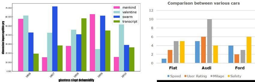
Data Extraction from Charts via Single Deep Neural Network

component λtext , λOM and λang balance each loss function           sification converges, weights in these three branches are
component. In our experiment, λtext is set to 0.1, and λOM          released to become trainable and their parameters are set
and λang are set to 1.                                              to the values provided in Section 3.2.5 and fixed until the
                                                                    end of training. While these fixing steps can be iterated, we
3.3. Inference                                                      observe that a single pass provides a good solution.
The inference approach for bounding box prediction and
                                                                    4.2. Training and Evaluation Data Generation
classification is outlined in (Ren & Sun, 2015), and the
inference approach for text prediction is specified in (Shi &       We utilize both simulated and public data sets because of the
Yao, 2017).                                                         limited availability of the latter. Matplotlib Python library is
                                                                    used to build the data set for bar and pie chart data extraction
Each chart is first recognized by the chart type classification
                                                                    models. To have varieties, we introduce randomness in
model to decide which data extraction model to use.
                                                                    colors for bar or pie, font sizes and types, orientations of
For a bar chart, each of its anchor proposals with confidence       texts, sizes of images as well as sizes of bars and pies. All
more than 0.8 is generated along with their text prediction         of the titles and x,y-axis labels are assumed to have less than
and class. Non-maximum suppression is employed to re-               three words from a vocabulary size of 25,000. Font type
move redundant proposals and the remaining proposals are            can be any one of 35 commonly used ones. Possible font
fed into the object-matching model to generate the final            size ranges for each type of text (titles, axis labels, tick and
prediction with inner relationship between proposals. There         legend labels) in a chart are set separately, and color choices
is still one last step for bar chart data extraction: linear in-    for bars and pies are arbitrary. Note that in the simulation
terpolation is employed to generate the value of a bar from         code we output all of the necessary ground truth information,
pixel locations to the y-axis value. The predicted values are       e.g., angles. For bar charts, tick mark and frame styles are
detected by the top boundary locations of bars.                     also considered with randomness. Each bar chart can be a
                                                                    single bar chart or a grouped one with up to five groups. In
Inference for a pie chart is slightly different. Since we
                                                                    terms of pie charts, the angle of the first right-center slice
assume that there is only one pie in a pie chart, we feed the
                                                                    boundary is random. The number of slices in our data set is
bounding box proposal (pie) with highest confidence after
                                                                    assumed to be less than 10.
non-maximum suppression into the angle prediction model.
The feature map of the pie is then rotated by each predicted        The bar chart data extraction model is trained only on our
angle to match with legend sample feature maps.                     simulated data set of 50,000 images due to the limitation of
                                                                    any public data set with annotations of bounding boxes for
4. Computational Study                                              bar charts. The annotations for ground truth include classes
                                                                    and bounding boxes for all objects, orientations and texts
In this section, we first illustrate the training strategies fol-   for textual objects, and object matching relations in charts.
lowed by the training and evaluation data generation process
                                                                    40,000 simulated pie charts are generated by the above
for the three deep learning models. Then we show the effec-
                                                                    strategy. Besides the annotations in bar charts, there is an
tiveness of our models by evaluating their performance on
                                                                    additional type of labels for boundary angles of slices, which
general test sets.
                                                                    starts from the right-center one and follows the counter-
                                                                    clockwise flow. The training data set also includes 10,000
4.1. Training Strategy                                              charts from the Microsoft FigureQA (Kahou & Bengio,
All of the chart type classification model and data extraction      2017) data set, so the training data set for the pie chart
models have the backbone of VGG16. We start from the                model consists of 50,000 images. FigureQA bar charts are
pre-trained ImageNet VGG16 weights as the first training            not used in training bar charts since they are too simple and
step.                                                               not diversified.

The second training step for chart type classification is to        The chart type classification model is trained on our sim-
train it on our simulated chart data set described in Sec-          ulated data set of 1,000,000 charts and fined-tuned on a
tion 4.2.                                                           data set consisting of 2,500 charts downloaded from Google
                                                                    Image. The simulated data set is generated by the Microsoft
In terms of the two chart data extraction models, the               Excel C# and Matplotlib Python library. The 2,500 chart
second training step focuses on the object detection and            images are downloaded from Google Image by using key-
classification branches. During this step, parameters               words “bar chart,” “pie chart” and labeled based on the cor-
λtext , λOM , λang are fixed to zero and the weights of these       responding keywords. We use them to fine-tune the model
corresponding branches are fixed to their initial random            in training.
values. After the training loss of object detection and clas-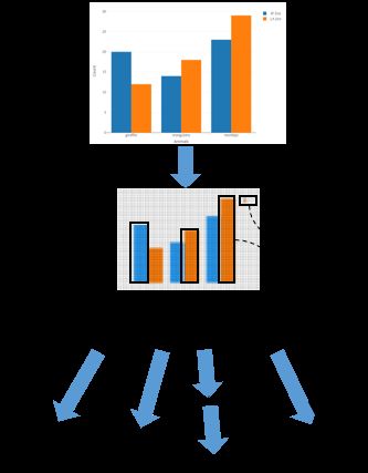
Data Extraction from Charts via Single Deep Neural Network
We use the same stragedy to generate the validation data
Table 1. Average Precision for each object in Simulated (Simul),
set of 5,000 bar chart images with annotations for the bar
FigureQA (FigQA) and human annotated (Annot) bar chart data
chart model. 4,000 simulated pie charts and 1,000 charts sets
from FigureQA data set are integrated as the validation data
set for the pie chart model. The validation data set for chart O BJECT S IMUL F IG QA A NNOT
type classification includes 5,000 simulated charts and 500
T ITLE 100.0 97.3 47.5
downloaded charts. X- AXIS LABEL 99.9 94.1 38.2
In order to show our models’ effectiveness, we consider Y- AXIS LABEL 90.9 93.5 75.0
X- TICK LABEL 91.0 85.0 48.1
the following test data sets: the first one called Simulated Y- TICK LABEL 88.1 91.3 75.4
is the data set with the same distribution as our training X- TICK LINE 89.4 0.0 58.2
data set and consisting of 3,000 charts in each setting; the Y- TICK LINE 87.5 87.0 76.5
second one for both bar and pie models is 1,000 charts LEGEND LABEL 90.8 100.0 75.1
from the FigureQA data set; the third one called Annotated LEGEND MARK 90.2 100.0 24.3
BAR 97.9 96.8 80.2
is 10 charts downloaded from Google Image and labeled M EAN 92.6 84.5 59.7
manually for each data extraction model; the last one called
Excel is generated by Microsoft Excel C# and consists of
1,000 charts for each model. reliable since the predicted value can slightly differ from
the ground truth. The lower y-tick label is the y-tick label
Regarding Excel C#, through their API we were not able
immediately below the actual value of the bar (and similarly
to figure out how to generate all of the necessary ground
defined upper y-tick label). Besides the 4-tuple, each bar
truth for training and thus they are not included in training
chart has its prediction of title, and x- and y-axis labels. All
data sets. In test evaluation, we only generate a subset of
the prediction results are summarized in Table 2.
ground truth labels and use them only for the corresponding
metrics. In Table 2, the accuracy of the entire “ALL” charts, titles,
and x-, y-axis labels in the first 4 rows represent the per-
4.3. Chart Type Classification centage of correctly predicted chart instances in each test
data set. In all elements consisting of text we count true
Our chart type classification model is based on VGG16. The positive only if all words match correctly. We define true
only difference is in the output layer, in which our model positive charts (”ALL”) as predicted with correct title, x-, y-
has two output categories, “bar chart” and “pie chart.” The axis labels and all 4-tuples with less than 1% error in value.
classification model achieves an accuracy of 96.35% on the The following 11 rows are based on each tuple prediction.
test data set of 500 images downloaded from Google. For example, the true positive instance for “tuple 10% err”
means the tuple is predicted with a less than 10% error in
4.4. Bar Chart Data Extraction value and the remaining 3 textual elements are completely
The effectiveness of the bar chart data extraction model is correct. The error is defined as:
first demonstrated by its object detection branch of the 10 |V aluepred − V alueGT |
categories. As shown in Table 1, the mean average precision Error = (8)
|V alueGT |
for the simulated test data set is 92.6%, which is higher than
84.5% for FigureQA and 59.7% for Annotated. Any of the where V alueGT is the ground truth value of each bar.
x-tick lines in the FigureQA data set are not detected since
The results show the model works well on Simulated, Fig-
the x-tick lines in the FigureQA charts are much longer than
ureQA and Excel bar chart data sets but not as good on the
our simulated ones. Legend marks in the Annotated data
Annotated data set.
set are also hard to detect since they have different styles or
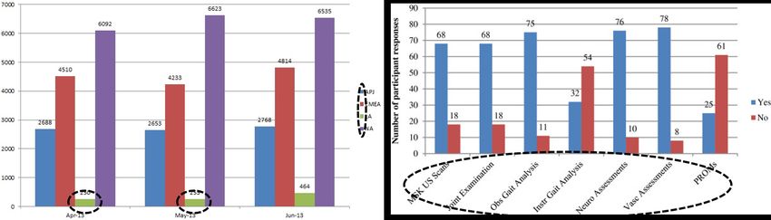
sizes from our training data set. We also plot six chart samples with “good,” “OK” or “bad”
predictions. “Good” samples are from true positives, while
To further evaluate the performance of the bar chart data ex-
“OK” samples predict some parts wrongly. “Bad” samples
traction model, we propose the following evaluation metric.
miss some important objects like bars or x-tick labels. The
We use a 4-tuple to represent the prediction of each bar in
model on the sample on the left in Figure 4b cannot detect
a bar chart: (x-tick label, value, lower y-tick label, upper
the entire 2-line title of more than 10 words since we do not
y-tick label). In the 4-tuple, x-tick label is matched to the
have such training samples, and the bar on the right chart
bar by the object matching branch (x-tick label can be either
cannot be detected correctly since the legend region covers
below the bar or in the legend), value is predicted using the
it. The left “bad” sample in Figure 4c has two very low bars
top boundary location of the bar. The introduction of the
and very small legend marks which are not detected by the
lower and upper y-tick labels makes the evaluation more
model. The right one has several long x-tick labels that are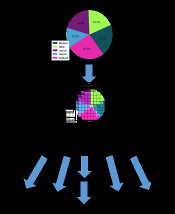
Data Extraction from Charts via Single Deep Neural Network

Table 2. Accuracy of bar chart prediction in Simulated (Simul),
FigureQA (FigQA), annotated (Annot) and Excel bar chart data
sets

  O BJECT             S IMUL    F IG QA    A NNOT     E XCEL
  ALL                   79.4       69.2       30.0      68.3
  T ITLE                95.6       94.8       40.0      91.0
                                                                  (a) Bar chart samples with “good” predictions, left from Simulated,
  X- AXIS LABEL         94.9       93.7       40.0      89.2
                                                                  right from Annotated
  Y- AXIS LABEL         88.2       93.0       50.0      83.1
  T UPLE 1% ERR         81.0       72.3       28.4      77.3
  T UPLE 5% ERR         83.4       76.2       32.8      79.2
  T UPLE 10% ERR        83.9       78.4       34.3      69.8
  T UPLE 25% ERR        85.6       81.3       38.8      83.4
  X- TICK LABEL         87.3       83.5       43.3      87.5
  L OWER VALUE          87.8       85.1       56.0      83.2
  U PPER VALUE          88.3       85.4       58.2      84.9
  VALUE 1% ERR          82.4       77.9       41.0      80.2
  VALUE 5% ERR          86.0       81.2       46.3      82.9      (b) Bar chart samples with “OK” predictions, left from Annotated,
  VALUE 10% ERR         87.7       83.4       50.0      83.3      right from Simulated
  VALUE 25% ERR         91.3       89.1       61.2      88.0

not detected correctly. These wrong predictions are mainly
caused by lack of variance in the training data set or the
convolution operations not working well on small objects.
A more accurate multi-line and multi-word text detection          (c) Bar chart samples with “bad” predictions, both from Annotated
and recognition model would improve the model. This can
be handled by augmenting the training data set. It is unclear     Figure 4. Bar chart samples with “good,” “OK” and “bad” predic-
how to improve the performance on small objects.                  tions; dash circles indicate problematic regions

4.5. Pie Chart Data Extraction
                                                                  when the slices have high contrast colors and they are not
Following similar evaluation metrics for bar charts, we first     too narrow. When there are slices with percentage of less
evaluate the average precision of 4 categories and their mean     than 2% (left sample in Figure 5b) or of similar color on its
value for pie charts in Table 3.                                  neighboring slice (right sample in Figure 5b), the model has
                                                                  difficulties handling it.
Compared with bar charts, objects in pie charts are much
easier to detect since there are fewer categories and the sizes
of objects are larger.                                            5. Conclusion
Different from bar charts, we define a 2-tuple to represent       In this paper, a system of neural networks is established to
the prediction of each slice in a pie chart, (legend, percent-    classify chart types and extract data from bar and pie charts.
age). The accuracy of our prediction results is shown in          The data extraction model is a single deep neural net based
Table 4. The error for pie charts is defined as:                  on Faster-RCNN object detection model. We have extended
                                                                  it with text recognition and object matching branches. We
               |P ercentagepred − P ercentageGT |                 have also proposed a percentage prediction model for pie
   Error =                                        .        (9)
                         P ercentageGT
The results show a great success on the FigureQA data set
since their pies have less variance and are included in our       Table 3. Average Precision for each object in Simulated (Simul),
training data set. The whole accuracy for the Annotated data      FigureQA (FigQA) and human annotated (Annot) pie chart data
set is much worse than the other two data sets because the        sets
accurate prediction of percentage of slices is hard, although
it gets a high accuracy of 77.8% for percentage prediction               O BJECT             S IMUL     F IG QA    A NNOT
in the Annotated data set with less than 5% errors.                      T ITLE               100.0      100.0       90.0
                                                                         P IE                 100.0      100.0      100.0
Figure 5 shows 4 pie charts from the Annotated data set                  LEGEND LABEL          98.9      100.0       83.3
which are divided into “good” and “bad” samples based                    LEGEND MARK           95.3      100.0       66.7
on the quality of the predictions. The model works well                  M EAN                 98.6      100.0       80.4
Data Extraction from Charts via Single Deep Neural Network
charts as another contribution. The model has been trained
on a simulated data set and performs successfully on 79.4%
of the simulated bar charts and 88.0% of the simulated
pie charts. The performance on the images downloaded
from Internet is worse than on the simulated data set or
another generated data set since it includes more variantions
not seen in training. Augmenting the training data set by
means of a more comprehensive simulation (or Microsoft
offering addition API functionality in Excel C#) is an easy
way to substantially improve the performance. It is more
challenging to find a way to cope with small objects.
(a) Pie chart samples with “good” predictions, from Annotated
Acknowledgements
This work was supported by Intel Corporation, Semiconduc-
tor Research Corporation (SRC).
References
Cliche, M., Rosenberg D. Madeka D. and Yee, C. Scatter-
act: Automated extraction of data from scatter plots. In
(b) Pie chart samples with “bad” predictions, from Annotated Joint European Conference on Machine Learning and
Knowledge Discovery in Databases, pp. 135–150, 2017.
Figure 5. Pie chart samples with “good” and “bad” predictions;
dash circles indicate challenging regions Girshick, R., Donahue J. Darrell T. and Malik, J. Rich fea-
ture hierarchies for accurate object detection and semantic
segmentation. In CVPR, pp. 580–587, 2014.
Girshick, R. Fast R-CNN. In CVPR, pp. 1440–1448, 2015.
Graves, A., Fernndez S. Gomez F. and Schmidhuber, J. Con-
nectionist temporal classification: labelling unsegmented
sequence data with recurrent neural networks. In ICML,
pp. 369–376, 2006.
He, K., Zhang X. Ren S. and Sun, J. Deep residual learning
Table 4. Accuracy of pie chart prediction in Simulated (Simul), for image recognition. In CVPR, pp. 770–778, 2016.
FigureQA (FigQA), annotated (Annot) and Excel pie chart data
sets Huang, J., Rathod V. Sun C. Zhu M. Korattikara A. Fathi A.
Fischer I. Wojna Z. Song Y. Guadarrama S. and Murphy,
K. Speed/accuracy trade-offs for modern convolutional
O BJECT S IMUL F IG QA A NNOT E XCEL object detectors. In CVPR, pp. 7310–7319, 2017.
ALL 88.0 98.5 20.0 68.6 Huang, W. and Tan, C.L. A system for understanding im-
T ITLE 96.4 100.0 60.0 92.5
T UPLE 1% ERR 90.0 98.5 28.9 71.2
aged infographics and its applications. In ACM Sympo-
T UPLE 5% ERR 90.5 99.0 57.8 75.3 sium on Document Engineering, pp. 9–18, 2007.
T UPLE 10% ERR 90.8 99.1 60.0 78.0
T UPLE 25% ERR 91.8 99.7 64.4 80.5 Jaderberg, M., Simonyan K. and Zisserman, A. Spatial
L EGEND 92.5 100.0 68.9 87.2 transformer networks. In NIPS, pp. 2017–2025, 2015.
P ERCENT 1% ERR 97.4 98.5 33.3 83.4
P ERCENT 5% ERR 97.8 99.0 77.8 88.9 Kahou, S.E., Atkinson A. Michalski V. Kdr . Trischler A.
P ERCENT 10% ERR 98.0 99.1 80.0 91.2 and Bengio, Y. Figureqa: An annotated figure dataset
P ERCENT 25% ERR 98.9 99.7 86.7 93.0 for visual reasoning. arXiv preprint arXiv:1710.07300,
2017.
Krizhevsky, A., Sutskever, I., and Hinton, G.E. Imagenet
classification with deep convolutional neural networks.
In NIPS, pp. 1106–1114, 2012.Data Extraction from Charts via Single Deep Neural Network Liu, W., Anguelov D. Erhan D. Szegedy C. Reed S. Fu C.Y. and Berg, A.C. SSD: Single shot multibox detector. In ECCV, pp. 21–37, 2016. Poco, J. and Heer, J. Reverse-engineering visualizations: Recovering visual encodings from chart images. In Com- puter Graphics Forum, pp. 353–363, 2017. Prasad, V. S. N., Siddiquie, B., Golbeck, J., and Davis, L. S. Classifying computer generated charts. In Content-Based Multimedia Indexing Workshop, pp. 85–92, 2007. Redmon, J., Divvala S. Girshick R. and Farhadi, A. You only look once: Unified, real-time object detection. In CVPR, pp. 779–788, 2016. Ren, S., He K. Girshick R. and Sun, J. Faster R-CNN: Towards real-time object detection with region proposal networks. In NIPS, pp. 91–99, 2015. Santoro, A., Raposo D. Barrett D.G. Malinowski M. Pas- canu R. Battaglia P. and Lillicrap, T. A simple neural network module for relational reasoning. In NIPS, pp. 4967–4976, 2017. Savva, M., Kong, N., Chhajta, A., Fei-Fei, L., Agrawala, M., and Heer, J. Revision: Automated classification, analysis and redesign of chart images. In Proceedings of the 24th Annual ACM Symposium on User Interface Software and Technology, pp. 393–402, 2011. Shi, B., Bai X. and Belongie, S. Detecting oriented text in natural images by linking segments. In CVPR, pp. 3482–3490, 2017. Shi, B., Bai X. and Yao, C. An end-to-end trainable neural network for image-based sequence recognition and its application to scene text recognition. In PAMI, pp. 2298– 2304, 2017. Siegel, N., Horvitz Z. Levin R. Divvala S. and Farhadi, A. Figureseer: Parsing result-figures in research papers. In ECCV, pp. 664–680, 2016. Simonyan, K. and Zisserman, A. Very deep convolutional networks for large-scale image recognition. In ICLR, 2012. Stewart, R., Andriluka M. and Ng, A.Y. End-to-end people detection in crowded scenes. In CVPR, pp. 2325–2333, 2016. Tian, Z., Huang W. He T. He P. and Qiao, Y. Detecting text in natural image with connectionist text proposal network. In ECCV, pp. 56–72, 2016. Zhou, Y. and Tan, C.L. Hough-based model for recognizing bar charts in document images. In SPIE, pp. 333–341, 2000.
You can also read