Predicting COVID-19 in very large countries: the case of Brazil - Research Square
←
→
Page content transcription
If your browser does not render page correctly, please read the page content below
Predicting COVID-19 in very large countries: the
case of Brazil
Vanderlei Cunha Parro1,*+ , Marcelo Lafetá1,+ , Felipe Ippolito1 , and Tatiana Natasha
Toporcov2
1 Instituto
          Mauá de Tecnologia, Electrical Engineering, São Caetano do Sul, 09580-900, Brazil.
2 Faculdade  de Saúde Pública da Universidade de São Paulo, São Paulo, 01246-904,Brazil.
* vparro@ieee.org
+ these authors contributed equally to this work

ABSTRACT

The existence of asymptomatic individuals with mild symptoms represents an additional challenge for the control of the
coronavirus disease 2019 (COVID-19) pandemic. This challenge puts pressure on public management officials involved in the
design of infrastructure for service provision as well as isolation procedures. The challenge is even greater in a country such
as Brazil, which has large physical dimensions with the assumption of free movement. Considering this scenario, this work
presents a new proposal for estimating health system use for COVID-19 cases, as well as a methodology for using the model in
the real world. The estimate was obtained by modifying the dynamic model known as Susceptible, Infected, Removed and
Dead (SIRD), including a parameter to model not all cases but only the health system dynamics. The model was tuned from
the data available for each state and updated day-by-day, establishing a figure of merit to assess the quality of the model and
determining the free parameters that best fit the model to the data. The proposed model and the respective tuned parameters
were validated considering the data available for the 26 Brazilian states, demonstrating strong adherence in most cases and
allowing the estimation of an epidemic model for the whole of Brazil, which was obtained via the linear combination of the
models for each state. In addition to the effective use of the health system, the incidence rate and removal rate were analysed,
as was the reproduction rate: baseline R0 and effective Rt . In the specific case of Brazil, the states that make up the federation
have autonomy in decision making, which increases the complexity of the analysis of the evolution of the pandemic. With the
proposed global model, the method used to tune the parameters and the available results, there was heterogeneity in the
dynamics observed for each state, which is compatible with some characteristics of the real-world scenario.

Introduction
In December 2019, the new coronavirus severe acute respiratory syndrome coronavirus 2 (SARS-Cov-2) was first identified in
Wuhan, China. On March 11, the World Health Organization designated COVID-19 as a pandemic. As of August 2020, more
than 23 million COVID-19 cases and 80,000 deaths had been reported worldwide1 . In Brazil, the virus was first identified in
São Paulo city on February 26, and the first death occurred in March in Rio de Janeiro. The new cases detected at the beginning
of the pandemic largely coincided with Brazilian cities with airport access, with approximately 2 million Brazilians exposed
in approximately 20 weeks. As of the 7th week after the first case, the virus had spread to cities without airports, probably
via road transport, increasing the population at risk. Within 5 weeks, according to Wesley Cotta/Ministry of Health data2 , all
Brazilian states had registered active cases of the disease. In addition to the different characteristics of the states, which have
HDI index values ranging from 0.631 for the state of Alagoas to 0.824 for the state of Distrito Federal, different measures were
taken to achieve social isolation, implying different courses of the pandemic.
    Brazil, with a population of approximately 200 million inhabitants, is composed of 26 states and the federal district.
Approximately 30 years ago, the country implemented a universal and decentralized health system (Sistema Único de Saúde)3 .
There was instability in the federal management of the health crisis caused by the pandemic, with a number of changes in
the Ministry of Health during a short period of time. States were independent in making several important decisions for
controlling the epidemic, leading to high heterogeneity in the non-pharmacological measures taken to mitigate the pandemic.
The occupation of the health system and decisions about isolation guidelines served as a guide for most of the official
communications from states (26) and municipalities (5570) in the Brazilian press4 .
    Internationally, machine learning has been widely used in an attempt to predict disease behaviour, with the aim of forecasting
demand for health services, as well as planning and evaluating measures to reopen quarantined sites5 ,6 ,7 . The choice of the
best model to forecast demand has been discussed in the literature and remains controversial. COVID-19 is a new disease,
and its transmission dynamics and natural history are not yet completely clear; in addition, there is a variable proportion of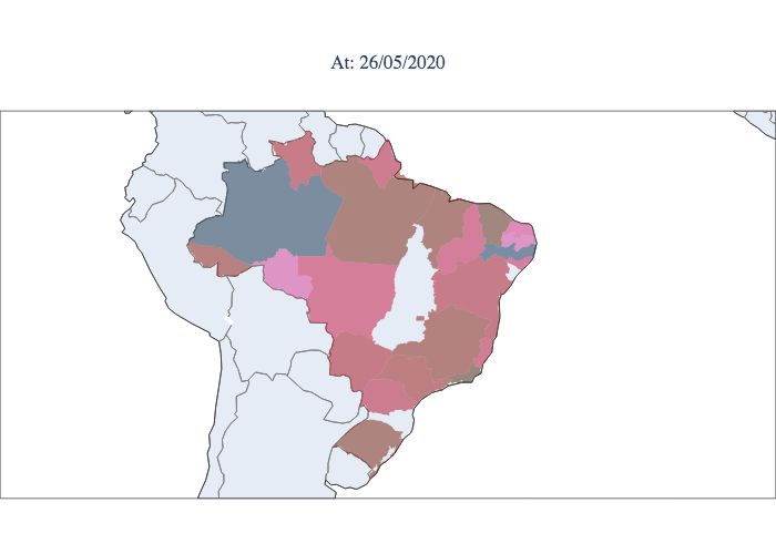
asymptomatic and mildly symptomatic individuals who are not notified and do not need treatment but transmit the disease8 .
This challenge is even greater in large countries with significant inequality and a heterogenous evolution of the pandemic, such
as Brazil. This country has high-quality data on COVID-19, which originate from the epidemiological surveillance of acute
influenza and respiratory syndromes and are available electronically.
    In this article, we propose a modification of the Susceptible, Infected, Removed, and Dead (SIRD)9 ,10 ,11 ,12 model to model
the dynamics of health system use based on reported cases and not on the epidemic as a whole13 . Its simplicity, when compared
to more complete and sophisticated models14 ,15 , makes it simpler to tune the model’s parameters as well as its use by public
agents in management and communication.Essentially, it is known from the characteristics of COVID-19 that only a portion of
those infected will use the health system. It is also known that the peak of the SIRD model is dependent on the population
considered. This logical implication led us to consider a weighting of the total population to estimate the use of the public
health system. The proposal was validated by applying the model to each Brazilian state. In the case of the model for each
state, tuning of the modified SIRD model allows a comparative assessment of its main parameters, infection rate and removal
rate, in addition to an assessment of the basic reproduction rate R0 and the effective reproduction rate Rt , which are all relevant
parameters for public management and decision making16 . The global model for all of Brazil was obtained from a linear
combination of the estimated active cases for each state. This proposal demonstrates that the behaviour of the epidemic in
Brazil does not follow the SIRD model and predicts that the epidemic will intensify in the second half of the year due to the
natural risk associated with its presence in different states and locations.

The model
In this section, the machine learning problem is introduced based upon the so-called SIRD model. With this particular
model structure, an optimization algorithm using a heuristic search is introduced into the learning algorithm. Additionally, a
data-driven optimization trick is introduced as a solution to the susceptible data unavailability problem by introducing a degree
of freedom to the algorithm. To start the optimization problem structure, we must acknowledge the SIRD differential model

      dS(t)      −β I(t)S(t)
               =             ,                                                                                                  (1)
        dt             P
       dI(t)     β I(t)S(t)
               =            − γI(t) − µI(t),                                                                                    (2)
        dt           P
      dR(t)
               = γI(t),                                                                                                         (3)
        dt
      dD(t)
               = µI(t),                                                                                                         (4)
        dt
    where β , γ and µ are the average number of contacts per person per period of time, the inverse of the number of days
required for a person to pass from the infected to the recovered state, and the average number of deaths per period of time.
Considering that the existing data sets are usually sampled uniformly, there is an advantage of using the discrete representation
of the SIRD model, which can be achieved by

       S(k + 1) = S(k) + ∆t −β I(k)S(k)/P ,                                                                                   (5)

        I(k + 1) = I(k) + ∆t β I(k)S(k)/P − γI(k) − µI(k) ,                                                                   (6)
      R(k + 1) = R(k) + ∆tγI(k),                                                                                                (7)
      D(k + 1) = D(k) + ∆tµI(k),                                                                                                (8)
where ∆t is the sample time of the data-sets, and P is the total population that should be considered for each case study.
    where ∆t is the sample time of the data sets and P is the total population that should be considered for each case study.
Note that from model equations 5 – 8, determining the mean squared error e(k + 1) of the model from the provided data is
straightforward. Therefore, it is possible to consider the error equation with an aggregated value for each component, such as
the maximum value of each component, resulting in the weighted error

                              2                                 2             2
                                                 2
                   S(k) − S̃(k)              ˜
                                      I(k) − I(k)      R(k) − S̃(k)    D(k) − S̃(k)
      e p (k) =                     +               +                +                ,                                         (9)
                          S                I                R               D
    where the components with the upper tilde are the output components of the differential model 5–8 for a particular set
                                              ˜ is the simulation of equation 6 for a particular set of parameters at k time
of parametersβ , γ and µ, e.g., the component I(k)

                                                                                                                              2/12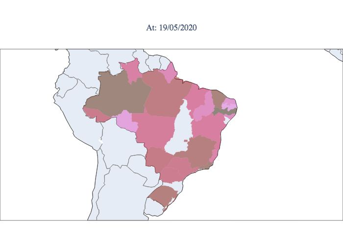
instants from the initial sample. From that, it is possible to compute the mean squared error as

                  ∑Nk=0 e(k)
      MSE =                                                                                                                  (10)
                      N
where N is the number of data samples.
    The defined MSE could be easily assumed as the cost function for the data-driven problem, but due to high amplitude
difference of the model components mean values, the cost function must take into consideration a pondering parameter. This
pondering parameter ensures the same importance for the error of each component of the model. This is not only interesting
because it equalizes the importance of all components on the cost function, but also it will enhance the backward and forward
stability of the optimization search space.
                                                      ˜
    Notice that to simulate the components, S̃(k), I(k),  R̃(k) and D̃(k), the learning algorithm must compute the equations 5–8
for a particular set of parameters, which is straightforward provided that the initial conditions I(0), R(0) and D(0), and a known
population of fixed size P,

      P = S(k) + I(k) + R(k) + D(k).                                                                                         (11)

Definition of susceptible component
The component of susceptible is usually not available on data-sets, and it is commonly computed based upon equation 11, using
the provided components I(k), R(k), D(k) and the estimated population size P. But this assumption is not quite accurate, since
not the entire population, P, should be considered susceptible, specially in case of COVID-19. The model will fit the data-set,
and the information provided by the data is actually the amount of people whom attended to a health care station, and then are
tracked by the data. In the next section, it will be discussed an algorithm capable of computing to extend the influence of the
susceptible component into the cost function, without compromising the learning space.
    Several studies suggest that the susceptible component should not be used in the optimization problem due to the imprecision
of the susceptible component, since one depend on several environment aspects such as isolation, disease health impact, targeted
people, and even climate conditions. This is quite problematic, since to predict the behavior of some characteristic points of the
epidemic, the initial value of the susceptible components is needed i.e. accordingly to 11, the value of the considered population
size. To exemplify, we could determine the susceptible component value at the time point where 2 is zero. So for that can write
2 when t = t p

      dI(t p ) β S(t p )I(t p )
              =                 − γI(t p ) − µI(t p ) , 0                                                                    (12)
        dt           P
where t p is the instant of t where the peak occurs. This leads to the following,

                  γ +µ
      S(t p ) =        P                                                                                                     (13)
                    β

which shows the peak moment t p as an unique realization directly depend on the correct selection of the population size, P. In
13, if provided a susceptible component value, computed from 11, and known population size P, the parameters β , µ and γ are
bounded by this particular representation. Now, consider that the correct initial value of the susceptible component, S(0), is not
the total population, but actually a proportion of it, λ P. This happens in scenarios where part of the population is immune or
are not affected impacted by the disease symptoms, and therefore they are only carries. In this particular case it is possible to
rewrite 13, as
                  γ +µ
      S(t p ) =        λ P.                                                                                                  (14)
                    β

Any distortion of the susceptible component, or of the population value, will be acknowledged by the new degree of freedom of
the model, λ . Which is ensured, since the previous parameters are guided by their particular components, 2–4, and the existent
data-set. The susceptible component, can be computed by considering λ , from 15. Considering the characteristics of CoViD 19,
where not all infectious people seek the health care system and that, our interest is to model the dynamics of the people who
attended to the health care system, mainly estimating its peak S(t p ), the weighting of the total population λ P allows the SIRD
model to be able to represent this dynamic.

      λ P = S(k) + I(k) + R(k) + D(k).                                                                                       (15)

                                                                                                                             3/12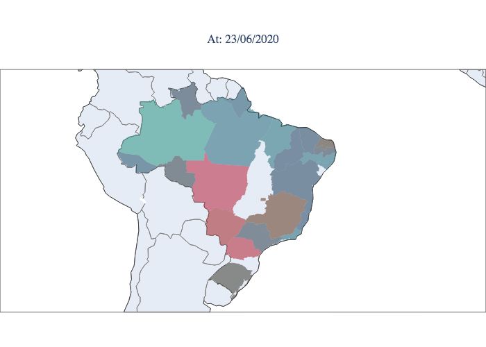
Optimization problem
The optimization problem can be structured in the form

                                ∑Nk=0 e p (k)
      arg {β ,γ,µ,λ }∈Ω min                                                                                                   (16)
                                    N
with e p (k) representing the pondered error at sample k, given by 9, and the component data reference of S(k) being achieved by
15. In order to suit the optimization scaffold of heuristic algorithms, the arguments must be bounded by the search space Ω.
    The search argument boundaries determination is straightforward once each parameter present a physical interpretation in
the model. Specifically, the parameters represent:
    • β , is the amount of people one contagious individual infects per time unit;
    • γ −1 , is the amount of time units that an infected individual takes to became recovered;
    • µ, is the proportion of infected people that dies per time unit;
    • λ , is the proportion of the population considered as initially susceptible.
And with no more than some references and common sense, it is possible to address the boundary limits for each of this
parameters. But there is an even better way to address this particular problem numerically. To understand this statement first we
must became familiar with the basic reproduction number, R0 , influence on the model. For this particular model, the R0 can be
obtained from the following relation
             βλ
      R0 =      .                                                                                                             (17)
              γ
    The basic reproduction number measures the average number of people, one contagious person will infect during it
contamination period. When R0 > 1, it shows that one person will infect more than one other, and therefore the disease will be
capable of sustaining its growth. In the complementary case, R0 < 1, the disease by itself will not have power to maintain a
growth to became an epidemic. And there is a vast bibliography that provides concrete knowledge on the value of R0 for the
most common epidemics. So here, we propose another approach for solving the optimization problem 16, where instead of
searching for the set of arguments {β , γ, µ, λ } we search for {R0 , D, µ, λ }, where D = γ −1 . Also, the search for R0 and D is
more conditioned then the search for β and γ, since R0 directly define the existence of the epidemic.
    The optimization problem can be rewritten in the form

                                 ∑Nk=0 e p (k)
      arg {R0 ,D,µ,λ }∈Ω̄ min                                                                                                 (18)
                                     N
where Ω̄ is the new search space, acknowledging R0 and D.

Validation for Brazilian states
Brazil is a large country, and there are several cultural and environmental aspects that make its states diverse. Each state could
be treated as an isolated epidemic environment, and we could fit a model for each individual state. Figure 1 shows the data and
the model predicted for two distinct Brazilian states, Maranhão and São Paulo. Using all data to fit each model, it is possible to
see that in scenarios where the data were collected rigorously and strict isolation was implemented, such as in Maranhão, as
expected, the algorithm was able to fit the data pattern with high fidelity. Furthermore, even in scenarios where the data were
not collected properly, such as São Paulo, the model was able to visualize the main pattern of the data.
    The modified SIRD model exhibited strong adherence to the data for most states with R2 values between 0.99 and 0.82.
Figure 1 illustrates the adjustment of the model for the date 7/21/20 for the state of Maranhão, which has a population of
approximately 7 million inhabitants (approximately 20 inhabitants perkm2 ) and declared 12 days of lockdown in May 2020,
and the state of São Paulo, which has a population of approximately 46 million inhabitants (approximately 166 inhabitants per
km2 ). The basic reproducibility index estimated for Maranhão was R0 = 3.52 and the basic reproducibility index estimated for
São Paulo was R0 = 4.78.
    In Figure 2, the R2 values for all states are presented for each scenario: searching for { R0 , D, µ, λ } and searching for
{ R0 , D, µ} with the previous setting = 1. From the results, it is possible to see that for all states, R2 is smaller when λ is
selected by the model, i.e., there is the degree of freedom in the population size. In addition, without the reduction of the
considered population, there is no possible set for the argument { R0 , D, µ} that can properly fit the analysed dataset. Note that
this fitness performance of the algorithm is only possible due to the new degree of freedom introduced in section .

                                                                                                                             4/12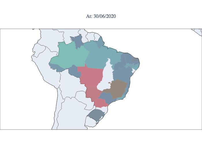
(a) Maranhão results.                                               (b) São Paulo results.

                 Figure 1. Comparison of predictions using the estimated models, with each state real data.

Results from the model
The global model for Brazil is determined via the linear combination of state models. The epidemic curve of active cases
,estimated on June 21, 2020, can be analysed in Figure 3. The peak observed in June 2020 is strongly influenced by the peak in
the state of São Paulo. The decay of the curve followed by support indicates that Brazil is expected to have a stable number
of active cases until September or October 2020 and an increasing number of active cases until the first quarter of 2021. An
important finding is that application of the SIRD model to Brazil as a whole (dotted in the figure) results in a different prediction
for the case dynamics, indicating control of the epidemic in October 2020. The simulation was carried out on 06/27/2020 and
the result clearly demonstrates that the model for Brazil does not follow the SIR model as well as, the proposed model, shows
more realistic behavior about the duration of the epidemic. Some models mistakenly predicted the end of the epidemic at the
end of August 202017 .
     In Figure 4, the predicted value for use of the Brazilian health system is presented, based on the average proportion of the
population that will attend hospitals and health centres throughout the epidemic. In Figure 4, this value is shown as more data
were provided to the model, i.e., as the epidemic developed in the country. It is interesting to note that the value becomes close
to the current (most recent) value of 1.0% of the population on 5/17/20, approximately 1.5 months before the first peak, when
the predicted use was 0.8% of the country’s population.
     It can also be seen in Figure 4 that the growth of the number of individuals seeking health care and its future predictions have
approximately linear behaviour, implying a constant growth rate, which indicates that the number of new cases is stable.Behavior
that is consistent when analyzed in the light of new cases and especially the number of deaths, approximately constant, which
tends to be more reliable. From the model’s point of view, this rate should drop starting in mid-October, as shown in Figure 3.

Results by state
One of the challenges of public health management was described as "flattening" the epidemic curve, a way to openly
communicate the strategies chosen for this purpose. Figure 5 illustrates the peaks in Brazil, with the first state to reach the peak
being Pernambuco and the last states to suffer from the acute phase of the epidemic being Mato Grosso and Mato Grosso do
Sul, which are located in the central west, and Paraná, which is located in the south. In Figure 6, the estimated parameters are
presented for the ten best adjusted states for the first scenario. From the table, it is possible to see that most values ofR0 stay in
this range, except for SC (Santa Catarina), indicating that the inclusion of the λ parameter helps with the parameter bias usually
observed in direct optimizations, where it is required that λ = 1.
    Considering the SIRD model for each state, it is observed that the recovery rate D for individuals who accessed the health
system is approximately 17 days and that the basic reproduction rateR0 is approximately 2.9. Two other relevant parameters are
the average mortality rate , which is close to 0.8%, which implies an estimated number of deaths of 128,000 in August 2020.
The rate of use of the average health system is on the order of 0.6% and may reach 1.0%, which implies an expectation that
2 million people will seek care in the health system. From Figure 6, it is possible to verify some other interesting features.
The first is related to the comparison analysis of the parameter D. In the data, a recovered person is not a person considered
to no longer be contagious but a person who has been cleared by the hospital as recovered from the disease. Therefore, the

                                                                                                                                5/12
Figure 2. R2 value comparing the predictions with the real data of each state and the reliability metric that shows the
proportion of the data that is reliable to use on the learning algorithm.

                                                                                            ,QIHFWHG GDWD
            N                                                                               &RXQWU\ ZLVH PRGHO SUHGLFWLRQ
                                                                                            6WDWH ZLVH PRGHOV SUHGLFWLRQV

            N

            N

            N

            N

            0DU         0D\          -XO         6HS         1RY          -DQ        0DU          0D\             -XO

                  Figure 3. Comparison of predictions using the estimated models, with each state real data.

state transfer dynamics, from infected to recovered, maps the time in which a person needs to receive health care until they are
considered no longer affected by the disease and thus cured. That is why the estimated parameters for D have an average value
of 17.97 when it is well known that a person is only contagious during their first week of symptoms. From the data, it was
defined that COVID-19 has a consistent value for the daily death rate, which has an average value of 0.6%. Compared with the
model results, the state that is most off is RJ, with an estimated value of 2.0%, but notice that this state that has the worst value
for R2 in Figure 2. This particular problem was caused by a lack of rigorous data collection. The data contain many outliers,
and during a long period of time, the data-set was not updated.The synthesis of the results, based on the models by state, can be
analyzed in Figure 7.

Space-time analysis
To calculate the Rt values for each Brazilian state, we used the predicted the number of infected individuals, considering a
window of w days. The prediction of the infection series can be estimated from the likelihood function considering a Poisson
process18 ,19 . This procedure can be applied to both raw data and data predicted by the model. The results are illustrated in
Figure 8 using a window w = 5 days displaced by 1 day, normalized by the z-score method. A second method, based on the

                                                                                                                                6/12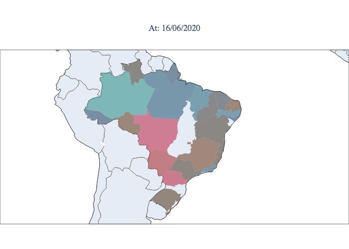
$SU           0D\           0D\            -XQ           -XQ            -XO           -XO

             Figure 4. Prediction of the proportion of the population to attend to health care systems in Brazil.

     Figure 5. Peak evolution of the epidemic in the Brazilian states illustrated in its temporal sequence of occurrence.

extraction of the β transmission rate, was applied for each state, resulting in a third estimate for control of the epidemic20 ,21 .
The results are also illustrated in Figure 8. This last method, although it is probably affected by the fluctuations in the updated
data, in addition to social isolation factors, is shown to be correlated with the other two. The estimate of the Rt rate from
the model works as a filter when compared to the rate obtained from the data window, indicating a species with an average
behaviour of Rt. As noted in Figures 1 and 8, there is a rapid recovery of the model from variations in the data. In the specific
case, the variation was caused by the variation of the data sources and their consolidation, but it is expected that the model

                                                                                                                              7/12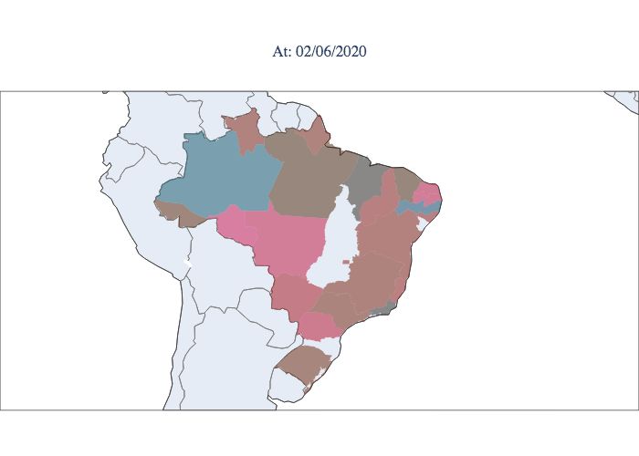
3( $0 5- 0$ 3$ 3( $0 5- 0$ 3$
$& $/ $3 &( 3– %$ $& $/ $3 &( 3– %$
(6 55 63 3% 52 56 (6 55 63 3% 52 56
51 0* ') 07 06 35 51 0* ') 07 06 35
(a) D - taxa de remoção em dias. (b) R0 - taxa básica de repordutividade.
Figure 6. Distributions of the estimated parameters D, R0 , µ and λ , for all Brazilian states based on the state that presented
the first peak. (a) Distribution of the estimated recovery rate in days: - D - X D = 17.97 ± σD = 3.41. (b) (b) Distribution of the
estimated basic reproductive rate: R0 - X R0 = 2.9 ± σR0 = 0.9.
recovery will be equally rapid if the change comes from real cases. In this sense, the rates estimated from data and from the
model can be used in a combined way for decision making, since they are interpreted on a 1- or 2-week horizon to observe
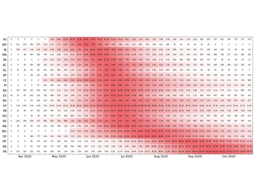
their effects. When we analyse the temporal and geographical progression of the virus, representing the effective reproductive
index Rt for each moment and each state, as shown in Figure 9, a considerable portion of the states are still observed to have
indexes greater than 1, and other states show a decline but are in the opening process. According to the graphs, it is notable
that the epidemic started in the northern and southeastern regions. Then, it spread progressively throughout the country but
did not progress proportionally in each state. The southeastern region does not reach its peak at the same time as the northern
region; it reaches its peak weeks later. Compared to the northern region, the southeastern region remains high Rt values at
present, showing less control of the epidemic. Note that at the moment, there are still three states that have Rt values greater
than 1.0, i.e., the epidemic is still growing. An example of this behaviour is the state of Paraná. As previously mentioned,
according to state models, Brazil will present a second smaller peak in September 2020. This second peak has an amplitude
mostly determined by infection numbers from the state of Paraná, which has the potential to reach values equivalent to those of
São Paulo (predominant state in the amplitude of the first peak).
8/12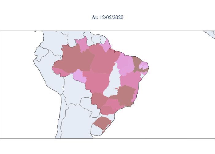
(a) D - removal rate in days.                               (b) R0 - Basal reproduction rate.

                    (c) µ - mortality rate.                              (d) λ - proportionality of the population.

Figure 7. Distributions of the estimated parameters D, R0 , µ e λ , accumulated since the beginning of the pandemic, for all
Brazilian states. (a) Distribution of the estimated recovery rate in days: D - X D = 17.97 ± σD = 3.41. (b) Distribution of the
estimated basic reproductive rate: R0 - X R0 = 2.9 ± σR0 = 0.9. (c) Distribution of the estimated mortality rate: µ -
X µ = 0.8% ± σµ = 0.2%. (d) Distribution of the proportionality rate of the estimated population: λ -
X λ = 0.6% ± σλ = 0.4%.

                                                 'DWD EDVHG                                                           'DWD EDVHG
                                                 7LPH YDULDQW                                                         7LPH YDULDQW
                                                 3UHGLFWLRQ EDVHG                                                     3UHGLFWLRQ EDVHG

                         7LPH GD\V                                                          7LPH GD\V
                 (a) Maranhão estimated R(t).                                      (b) São Paulo estimated R(t).

                      Figure 8. Comparison of standard scaled Rt from different estimate algorithms.

                                                                                                                                  9/12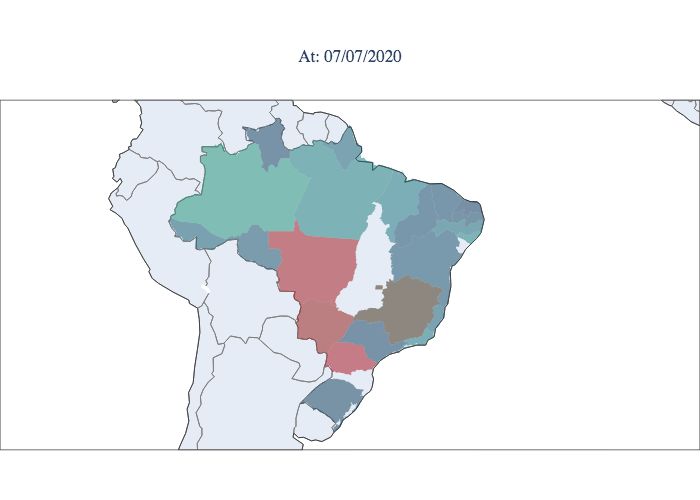
Figure 9. Estimated values of Rt for each state during the epidemic period in Brazil. Starting in March 2020 (upper left
corner) and concluding in September 2020 (lower right corner).

Conclusion
In conclusion, our modified SIRD model allowed the estimation of the COVID-19 epidemic model for the whole Brazil and
may be used in other very large countries, such as USA, India and Russia. When predicting the future of the pandemic in those
countries, it is important that local variation in epidemic stage is accounted in the model to provide accurate. results.The use of
the composite model, to understand the epidemic in Brazil, allowed for a more realistic modeling, regarding the predictions of
the use of the health system, as well as the average control parameters of the epidemic. We also found that COVID-19 peaked
in Brazilian states during periods in which the peak of respiratory diseases also used to occur. The values of R0 and Rt higher
than 1 found for Brazilian States and the high values predicted until the last quarter of 2020 suggests that non-pharmacological
measures will be still needed for months.

                                                                                                                             10/12
References
1. Dong, E., Du, H. & Gardner, L. An interactive web-based dashboard to track COVID-19 in real time, DOI: 10.1016/
S1473-3099(20)30120-1 (2020).
2. Cota, W. Monitoring the number of COVID-19 cases and deaths in Brazil at municipal federative units level. Scielo Prepr.
(2020).
3. Massuda, A., Hone, T., Leles, F. A. G., De Castro, M. C. & Atun, R. The Brazilian health system at crossroads: Progress,
crisis and resilience. BMJ Glob. Heal. 3, 1–8, DOI: 10.1136/bmjgh-2018-000829 (2018).
4. de Souza, W. M. et al. Epidemiological and clinical characteristics of the early phase of the COVID-19 epidemic in Brazil.
medRxiv - Imp. Coll. Lond. 19, DOI: 10.1101/2020.04.25.20077396 (2020).
5. Adam, D. Special report: The simulations driving the world’s response to COVID-19, DOI: 10.1038/d41586-020-01003-6
(2020).
6. Nikolopoulos, K., Punia, S., Schäfers, A., Tsinopoulos, C. & Vasilakis, C. Forecasting and planning during a pandemic:
COVID-19 growth rates, supply chain disruptions, and governmental decisions. Eur. J. Oper. Res. DOI: 10.1016/j.ejor.
2020.08.001 (2020).
7. Jo, H., Son, H., Jung, S. Y. & Hwang, H. J. Analysis of COVID-19 spread in South Korea using the SIR model with
time-dependent parameters and deep learning. medRxiv 2020.04.13.20063412, DOI: 10.1101/2020.04.13.20063412 (2020).
8. Ahmad, A. et al. The Number of Confirmed Cases of Covid-19 by using Machine Learning: Methods and Challenges.
Arch. Comput. Methods Eng. DOI: 10.1007/s11831-020-09472-8 (2020). 2006.09184.
9. Chen, Y.-C., Lu, P.-E., Chang, C.-S. & Liu, T.-H. A Time-dependent SIR model for COVID-19 with Undetectable Infected
Persons. 1–18 (2020). 2003.00122.
10. Tuckwell, H. C. & Williams, R. J. Some properties of a simple stochastic epidemic model of SIR type. Math. Biosci. 208,
76–97, DOI: 10.1016/j.mbs.2006.09.018 (2007).
11. Weiss Sir Ronald Ross, H. The SIR model and the Foundations of Public Health. MATerials MATemàtics Vol. 17,
1887–1097 (2013).
12. Huang, W. & Provan, G. An improved state filter algorithm for SIR epidemic forecasting. Front. Artif. Intell. Appl. 285,
524–532, DOI: 10.3233/978-1-61499-672-9-524 (2016).
13. Bonneville, F., Wallinga, J. & Fiocco, M. BAYESIAN FORECASTING OF Specialisation : Statistical Science STATISTI-
CAL SCIENCE Basis huisstijl. (2019).
14. Giordano, G. et al. Modelling the COVID-19 epidemic and implementation of population-wide interventions in Italy,
vol. 26 (Springer US, 2020).
15. D’Arienzo, M. & Coniglio, A. Assessment of the SARS-CoV-2 basic reproduction number, R0, based on the early phase
of COVID-19 outbreak in Italy. Biosaf. Heal. 2, 57–59, DOI: 10.1016/j.bsheal.2020.03.004 (2020).
16. Adam, D. A guide to R - the pandemic’s misunderstood metric, DOI: 10.1038/d41586-020-02009-w (2020).
17. Filho, L. R. & Lichtenthäler, D. G. A dynamic model for Covid-19 in Brazil. Medrxiv 1–10, DOI: 10.1101/2020.05.10.
20097550 (2020).
18. Chowell, G., Hyman, J. M., Bettencourt, L. M. & Castillo-Chavez, C. Mathematical and statistical estimation approaches
in epidemiology. Math. Stat. Estim. Approaches Epidemiol. 1–363, DOI: 10.1007/978-90-481-2313-1 (2009).
19. Nishiura, H. Correcting the actual reproduction number: A simple method to estimate R0 from early epidemic growth data.
Int. J. Environ. Res. Public Heal. 7, 291–302, DOI: 10.3390/ijerph7010291 (2010).
20. Pollicott, M., Wang, H. & Weiss, H. Extracting the time-dependent transmission rate from infection data via solution of an
inverse ODE problem. J. Biol. Dyn. 6, 509–523, DOI: 10.1080/17513758.2011.645510 (2012).
21. Pollicott, M., Wang, H. & Weiss, H. Extracting the time-dependent transmission rate from infection data via solution of an
inverse ODE problem. J. Biol. Dyn. 6, 509–523, DOI: 10.1080/17513758.2011.645510 (2012). 0907.3529.
Acknowledgements (not compulsory)
The authors would like to thank the Instituto Mauá de Tecnologia for funding this work.
11/12Author contributions statement
Vanderlei Cunha Parro established the methodology and evaluated the model results, Marcelo Lafetá and Felipe Ipólito
developed the Python code and all interfaces, and Tatiana Natasha Toporcov revised the results from the epidemiological
perspective. All authors reviewed the manuscript.
Additional information
The developed system is available on an open platform that can be accessed at https://epidemicapp-280600.web.
app/. On this platform, it is possible to submit a standard csv file and receive a synthesis report, synchronized model and
python source code. Complete documentation can be found at https://epidemicmodels.readthedocs.io/en/
latest/. The data used for tuning the model and generating the results were obtained from https://wesleycota.
com/.
12/12You can also read