Scattering efficiencies measurements of soft protons at grazing incidence from an Athena Silicon Pore Optics sample
←
→
Page content transcription
If your browser does not render page correctly, please read the page content below
Noname manuscript No.
                                              (will be inserted by the editor)

                                              Scattering efficiencies measurements of soft protons
                                              at grazing incidence from an Athena Silicon Pore
                                              Optics sample

                                              Roberta Amato · Sebastian Diebold ·
                                              Alejandro Guzman · Emanuele Perinati ·
                                              Chris Tenzer · Andrea Santangelo ·
                                              Teresa Mineo
arXiv:2110.04122v1 [astro-ph.IM] 8 Oct 2021

                                              Received: date / Accepted: date

                                              Abstract Soft protons are a potential threat for X-ray missions using grazing
                                              incidence optics, as once focused onto the detectors they can contribute to
                                              increase the background and possibly induce radiation damage as well. The
                                              assessment of these undesired effects is especially relevant for the future ESA
                                              X-ray mission Athena, due to its large collecting area. To prevent degradation
                                              of the instrumental performance, which ultimately could compromise some of
                                              the scientific goals of the mission, the adoption of ad-hoc magnetic diverters is
                                              envisaged. Dedicated laboratory measurements are fundamental to understand
                                              the mechanisms of proton forward scattering, validate the application of the
                                              existing physical models to the Athena case and support the design of the
                                              diverters. In this paper we report on scattering efficiency measurements of
                                              soft protons impinging at grazing incidence onto a Silicon Pore Optics sample,
                                              conducted in the framework of the EXACRAD project. Measurements were
                                              taken at two different energies, ∼470 keV and ∼170 keV, and at four different
                                              scattering angles between 0.6° and 1.2°. The results are generally consistent
                                              with previous measurements conducted on eROSITA mirror samples, and as
                                              expected the peak of the scattering efficiency is found around the angle of
                                              specular reflection.

                                              Roberta Amato
                                              Dipartimento di Fisica e Chimica - Emilio Segré, Università degli Studi di Palermo, via
                                              Archirafi, 36, 90123 Palermo, Italy
                                              INAF-IASF Palermo, via Ugo La Malfa, 153, 90146 Palermo, Italy
                                              IAAT, University of Tübingen, Sand 1, 72076 Tübingen, Germany
                                              E-mail: astro.roberta@gmail.com
                                              Sebastian Diebold · Alejandro Guzman · Emanuele Perinati · Chris Tenzer · Andrea San-
                                              tangelo
                                              IAAT, University of Tübingen, Sand 1, 72076 Tübingen, Germany
                                              Teresa Mineo
                                              INAF-IASF Palermo, via Ugo La Malfa, 153, 90146 Palermo, Italy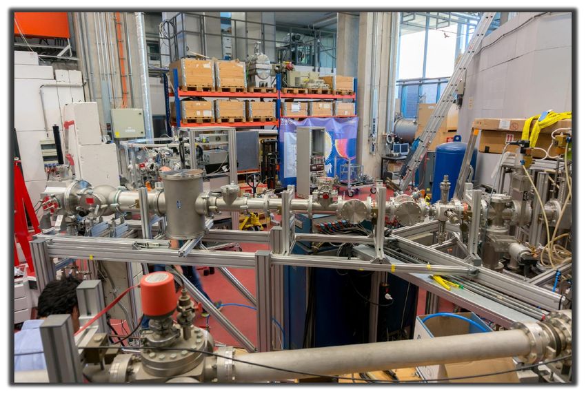
2                                                                  Roberta Amato et al.

Keywords Soft protons · X-ray background · proton scattering · grazing
incidence angle · X-ray astronomy

1 Introduction

Orbiting X-ray observatories are subjected to the impact of charged particles
of different origins, e.g. cosmic rays, solar wind and solar events, electrons and
protons trapped in the Earth magnetosphere, etc. Amongst them, protons with
typical energies ranging from a few tens to a few hundreds of kiloelectronvolts,
the so-called ‘soft protons’ (SP), are scattered and funneled towards the focal
plane when impinging at grazing incidence on X-ray optics. Once they reach
the instruments at the focal plane, they significantly contribute to the level
of non-X-ray background (NXB), and potentially damage the detectors in the
most severe cases. The effects of SP were first observed on the Chandra X-
ray Observatory (Weisskopf et al. 2000) and on XMM-Newton (Jansen et al.
2001), both launched in 1999. To this day SP affect the operability of these
X-ray missions by significantly reducing their useful observing time and their
duty cycles – for instance, the observing time of XMM-Newton is reduced by
∼30–40 % (Ghizzardi et al. 2017).
     SP constitute an even bigger issue for Athena (Advanced Telescope for High
Energy Astrophysics, Nandra et al. 2013), an L-class ESA mission, planned to
be launched in the early 2030s. The telescope will be equipped with Silicon
Pore Optics (SPO) (Willingale et al. 2013), wafers of silicon coated with high-
Z materials, stacked one upon the other and arranged to cover the whole pupil
of the telescope.
     Athena will orbit around the second Lagrangian point L21 of the Earth-Sun
system, at a distance of about 1.5 million kilometer from Earth in the anti-
Sun direction. This orbit lies in the tail of the Earth magnetosphere, where the
particle environment is extremely variable (Lotti et al. 2017). At present, the
science driven requirement for SP is that their flux at the focal plane has to
be < 5 × 10⁻⁴ cts s−1 cm−2 keV−1 (corresponding to 10 % of the total NXB),
in the 2–10 keV energy band, for 90 % of the observing time2 . In order to have
a thorough estimate of the SP flux expected at the focal plane, knowing the
scattering efficiency of soft protons at grazing incidence from Athena’s SPO
is fundamental. To achieve this goal, we performed experimental scattering
efficiency measurements with a SPO sample.
     Similar experimental measurements have already been performed for XMM-
Newton (Rasmussen et al. 1999) and eROSITA (Diebold et al. 2015, 2017)
mirror samples. Especially the measurements on eROSITA showed that the
scattering is always non-elastic, with energy losses of the order of a few tens
of kiloelectronvolts, depending on the energy of the incident beam. The scat-
tering efficiency always peaks close to the angle of specular reflection and is
  1 Currently, there are strong suggestions in favour of an L1 orbit, where the particle

environment is better known, though highly variable
  2 https://www.cosmos.esa.int/documents/400752/507693/Athena_SciRd_iss1v5.pdf
Scattering efficiencies of soft protons from Athena SPO                         3

higher for lower incident angles, while it is almost independent of the energy
of the impinging protons.
    A model for the scattering efficiency of ions at grazing incidence from the
surface of a material was developed by Remizovich et al. (1980), in non-elastic
approximation. However, the model is generally valid for any surface and con-
tains some approximations, therefore a simple application of the Remizovich
formula to the eROSITA data did not exactly reproduce the efficiencies mea-
sured in the laboratory (Amato et al. 2020). A fit of the experimental data
with the Remizovich formula led to the evaluation of the parameter enclosing
the micro-physics of the scattering, so that a new analytical semi-empirical
model that better reproduces the data from the eROSITA mirror sample was
derived (Amato et al. 2020). This model can be used to assess the SP flux
expected at the instrumental focal plane of the satellite. The model can also
be applied to Athena, provided that the proton scattering properties of the
SPO are experimentally determined.
    In this publication, we present the first measurements of scattering efficien-
cies of low-energy protons off a SPO sample. These experimental activities were
conducted in the framework of the EXACRAD (Experimental Evaluation of
Athena Charged Particle Background from Secondary Radiation and Scatter-
ing in Optics) project funded by ESA. The paper is structured as follows: we
first describe the laboratory setup and the elements along the beam line in
Sect. 2; in Sect. 3 we illustrate how the scattering efficiency is derived from
the raw data; the new data are presented in Sect. 4 and are compared to the
data from eROSITA as well as to the semi-empirical model mentioned above
in Sect. 9; finally, we draw our conclusions in Sect. 5.

2 Experimental setup

The experiment was conducted at the 2.5 MV Van de Graaff accelerator at the
Goethe University (Riedberg Campus) in Frankfurt am Main. The setup of
the beamline, similar to that of Diebold et al. (2015, 2017), is given in Figs. 1,
2, and 3.

2.1 Beamline setup

Protons enter the beamline through a copper pinhole aperture of the diame-
ter of 1 mm, which reduces the size of the incoming beam to prevent pile-up
and to maintain reasonable rates on the detectors. Successively, the beam goes
through a 0.002 mm thick aluminium foil, which degrades the incoming beam
energy below the lower limit of the accelerator. The degraded beam enters, at
this point, a 78 cm long collimator, which directs part of the widened beam
directly to the target. Two further apertures are positioned at the entrance
and at the exit of the collimator, both with a diameter of 1 mm. This diam-
eter limits the smallest possible incident angle to ∼0.5◦ . The apertures are
4 Roberta Amato et al.
Detectors
(PIPS)
Beam direction
Target chamber
Pinhole h
aperture
Collimator
✓0
✓
d
Degrader
foil (Al) Normalisation Detector chamber
detector (PIPS)
Fig. 1 Schematic drawing (not in scale) of the beamline setup. The proton beam enters
the setup from the left-hand side. It encounters the pinhole aperture (1 mm in diameter),
the Al degrader foil (0.002 mm thick) and the collimator. Inside the target chamber, the
normalisation detector can be lowered down to intercept the beam for the normalisation
measurements. If the normalisation detector is not in the line of the beam, then protons are
reflected from the SPO sample (in yellow) towards the detector chamber, where they hit the
central and lateral detectors. The incident angle θ0 between the line of the beam and the
mirror varies with the inclination of the target plate, while the scattering angle θ between
the mirror and the detectors in the detector chamber varies with the their height h. The
distance d between the target plate and the vertical ax of the central detectors is fixed to
942 mm.
Fig. 2 A CAD model of the beamline (same as Diebold et al. 2015). The proton beam
enters the setup from the right and moves towards the left. The SPO sample is located in
the target chamber, while the detector is placed in the chamber at the end of the beamline
(detector chamber). A second detector (not shown in the picture) was placed next to the
central one, with an angular distance of ∼ 2◦ .
supported in their position by 2 mm aluminum plates, which absorb any pro-
ton of the degraded beam not entering the apertures and being scattered by
the inner walls of the collimator and of the beamline itself.
The SPO target (Fig. 4), provided by cosine 3 , consists of a 110 mm long
single silicon wafer, 0.775 mm thick, grooved in the bottom, and coated on
3 https://www.cosine.nl/cases/silicon-pore-optics-mirror-modules-spo-for-astronomy/.Scattering efficiencies of soft protons from Athena SPO 5
Detector Target
chamber chamber Degrader
foils
Collimator
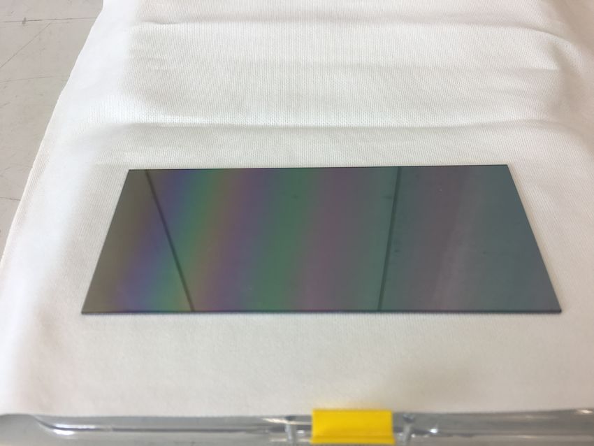
Fig. 3 Picture of the beamline at the Van der Graaff accelerator facility. The beam direction
is from the right to the left. The position of the degrader foils and the collimator inside the
beamline are pointed out, as well as the detector and target chambers.
Fig. 4 Pictures of the SPO sample, with the reflecting surface up (left) and down (right).
top with a 10 nm of iridium and 7 nm of silicon carbide4 . It is located in an
apposite chamber (hereafter called target chamber) and mounted on a tiltable
plate. The height of the target can be adjusted by a set of screws underneath
the plate. A linear manipulator is used to change the inclination of the plate,
i.e., of the incident angle (θ0 ). The pivoting point is is several centimeters
below the line of the beam, so that the target can be completely removed from
the beam, allowing for a determination of the primary beam position on the
detector plane. The manipulator is set below the target chamber and hence
can be easily accessed when the system is under vacuum.
4 Though iridium is the baseline coating material, a low-Z overcoating is also considered
to improve the reflectivity at lower energies. Different low-Z materials and thicknesses are
currently under investigation.6 Roberta Amato et al.
Between the exit of the collimator and the target plate, a Passivated Im-
planted Planar Silicon (PIPS) detector5 is mounted on a push-pull manipu-
lator, at the same height of the beamline. This detector is used to register
the amount of flux of the incident beam impinging on the target, useful to
have normalisation measurements. This detector will be called hereafter ’nor-
malisation detector’. The push-pull manipulator permits a fast removal of the
detector, guaranteeing a measure of the impinging proton flux (Φinc , cfr. Eq. 2)
for each measure of the scattered beam (see Sect. 3 for the need of having fre-
quent normalisation measurements). An aluminium blind with an aperture of
3 mm is set on top of the normalisation detector to avoid saturation. Lastly,
downstream of the target chamber, a thick aluminum sheet, with a slit of 3 cm
height and 1 cm width, is installed a few centimeters after the target plate.
This window lets pass only the protons on the line of the beam, while the
sheet absorbs all the ones that have been scattered by the inner walls or by
the other elements in the target chamber.
At the end of the beamline, a second chamber (hereafter detector chamber)
hosts two more PIPS detectors, called ‘central detector’ and ‘lateral detector’,
respectively, used to register the on-axis and off-axis fluxes (Φscat (θ0 , θ, φ), cfr.
Eq. 2) of the beam scattered by the target. They are mounted on a second
linear manipulator, which allows a spatially resolved sampling of the scattered
beam. The distance between the center of the target plate and the detection
plane is 942 mm. The central detector is aligned with the beam, while the
lateral detector is set on the left. This configuration allows for a coverage of
the scattered beam on the the incident direction and at an azimuthal angle φ
of 1.97◦ ± 0.13◦ . On top of each detector there is a blind with an aperture of a
diameter of 1 mm for the central detectors and of 3 mm for the lateral detector,
respectively. They reduce the solid angle of the detectors with respect to the
mirror center to about 8 × 10⁻⁷ sr and 2 × 10⁻⁵ sr for the central and lateral
detector, respectively.
2.2 Data acquisition chain
The pulse signal produced by the PIPS is amplified and digitalised trough
several analogical/digital electronic components. A flow chart is given in Fig. 5.
The PIPS detectors produce a pulse with an amplitude proportional to the
energy of the incident particle. The pulse signal from each PIPS goes through
its own pre-amplifier and amplifier and it is then digitalised by the Analog
to Digital Converter (ADC). The ADC receive the continuous signal (from
0 to ∼10 V) from the three channels – one for each detector – and convert
them into discrete signals, distributing it into 8192 bins, with a resolution of
1.22 mV. The digitised signals are then passed to the histogramming memory,
which produces an histogram for each channel. Once the measurement is done,
5 The PIPS detectors used in this experiment have a nominal depletion region of 0.1 mm
and a lower energy threshold of a few tens of keV.Scattering efficiencies of soft protons from Athena SPO 7
the histograms are read out by the CAMAC module and are transferred to a
computer, which acquires and stores them as raw data files.
The process of digitalisation of the data within the ADC takes a certain
time (fractions of seconds), so that if a new signal comes within that time,
it is not registered. To account for this dead-time, a pulse generator, which
generates pulses at a fixed frequency, is connected to the ADC and to a scaler,
which counts the number of pulses produced by the pulse generator during the
acquisition time. The scaler is also fed to the CAMAC control module. The
difference between the reading of the counts from the ADC and that from the
scaler gives the dead-time correction factor (cfr. Eq. 4). The pulse generator
fed to the ADC constitutes another channel, so that the whole acquisition
systems consists of four channels, all working simultaneously, and the scaler.
Pre-Amp Amp
Pre-Amp Amp
Histogramming
Pre-Amp Amp ADC
Memory
Pulse Generator
CAMAC
Scaler Acquisition Computer
Controller
Fig. 5 Data flow of the electronic chain for the acquisition of the experimental data. The
analogical signal from the PIPS detectors first goes through a pre-amplifier and an ampli-
fier, then it is converted into a digital signal by the ADC, and finally it is stored in the
histogramming memory. Contemporary, a pulse genarator sends signal at a fixed frequency
to the ADC and to a scaler. The digitised signals are read out by a CAMAC controller unit,
which transmits them to a computer once the measurement is finished.
2.3 Alignment and angular calibration
The alignment of all the movable elements on the beamline, i.e., the pinhole
aperture, the slits, the normalisation detector, and the central detector, is done
by using a telescope previously aligned with the exit of the accelerator.
A 520 nm laser is employed to perform the angular calibration. The laser
is set right after the pinhole aperture and goes through all the slits. When
the target plate is down, the laser reaches the central detector in the detector
chamber. In this way, the zero of the beamline, corresponding to θ = 0◦ , can
be established. This measurement gives also the vertical offset on the linear
manipulator of the central/lateral detectors.
To calibrate the incident and scattering angles, we use the property of the
mirror target to reflect optical light. Hence, we raise the target plate, using its8 Roberta Amato et al.
own manipulator, until the light is blocked. Then, we raise the central detector
till the laser beam is detected again. Assuming a specular reflection, the angle
subtended by the height h of the manipulator will be ζ = θ + θ0 = 2θ0 , so that
the incident angle can be computed as:
ζ
θ0 = (1)
2
This operation is repeated several time, so that we end up with different an-
gles corresponding to different readings on the linear manipulator of the target
plate. The incident angle can then be determined with a simple linear inter-
polation.
3 Efficiency definition and normalisation measurement
y
AAAB83icdVDLSgNBEJyNrxhfUY9eBoPgadnVoMkt6MVjAuYByRJmJ504ZPbBTI8QlnyBVz15E69+kAf/xd01gs86FVXddHX5sRQaHefVKiwtr6yuFddLG5tb2zvl3b2Ojozi0OaRjFTPZxqkCKGNAiX0YgUs8CV0/ell5ndvQWkRhdc4i8EL2CQUY8EZplJrNixXHLtarzmndfqbuLaTo0IWaA7Lb4NRxE0AIXLJtO67ToxewhQKLmFeGhgNMeNTNoF+SkMWgPaSPOicHhnNMKIxKCokzUX4upGwQOtZ4KeTAcMb/dPLxL+8vsFxzUtEGBuEkGeHUEjID2muRNoA0JFQgMiy5EBFSDlTDBGUoIzzVDRpJaW0j8+n6f+kc2K7Z3a1Va00LhbNFMkBOSTHxCXnpEGuSJO0CSdA7sg9ebCM9Wg9Wc8fowVrsbNPvsF6eQcen5Hu
AAAB9nicbVC7TsNAEDyHVwivACXNiQiJKrIRAsoIGsogkYeUWNH5sklOOZ9Pd2tEZOUXaKGiQ7T8DgX/gm1cQMJUo5ld7ewEWgqLrvvplFZW19Y3ypuVre2d3b3q/kHbRrHh0OKRjEw3YBakUNBCgRK62gALAwmdYHqT+Z0HMFZE6h5nGvyQjZUYCc4wk/p6IgbVmlt3c9Bl4hWkRgo0B9Wv/jDicQgKuWTW9jxXo58wg4JLmFf6sQXN+JSNoZdSxUKwfpJnndOT2DKMqAZDhaS5CL83EhZaOwuDdDJkOLGLXib+5/ViHF35iVA6RlA8O4RCQn7IciPSEoAOhQFEliUHKhTlzDBEMIIyzlMxTluppH14i98vk/ZZ3buon9+d1xrXRTNlckSOySnxyCVpkFvSJC3CyYQ8kWfy4jw6r86b8/4zWnKKnUPyB87HN8Nvks0=
✓
AAAB+HicbVC7TsNAEDyHVwivACXNiQiJKrJRBJQRNJRBIg8psaL1ZZMcOT90t0YKVv6BFio6RMvfUPAvOMYFJEw1mtnVzo4XKWnItj+twsrq2vpGcbO0tb2zu1feP2iZMNYCmyJUoe54YFDJAJskSWEn0gi+p7DtTa7nfvsBtZFhcEfTCF0fRoEcSgGUSq0ejZGgX67YVTsDXyZOTiosR6Nf/uoNQhH7GJBQYEzXsSNyE9AkhcJZqRcbjEBMYITdlAbgo3GTLO2Mn8QGKOQRai4Vz0T8vZGAb8zU99JJH2hsFr25+J/XjWl46SYyiGLCQMwPkVSYHTJCy7QG5AOpkQjmyZHLgAvQQIRachAiFeO0l1Lah7P4/TJpnVWd82rttlapX+XNFNkRO2anzGEXrM5uWIM1mWD37Ik9sxfr0Xq13qz3n9GCle8csj+wPr4BXSqTtg==
✓0
AAAB+3icbVC7TsNAEDyHVwivACXNiQiJKrIRAsoIGsogkQdKrGh92SSnnB+6WyNFVr6CFio6RMvHUPAv2MYFJEw1mtnVzo4XKWnItj+t0srq2vpGebOytb2zu1fdP2ibMNYCWyJUoe56YFDJAFskSWE30gi+p7DjTW8yv/OI2sgwuKdZhK4P40COpABKpYc+TZBgYFcG1Zpdt3PwZeIUpMYKNAfVr/4wFLGPAQkFxvQcOyI3AU1SKJxX+rHBCMQUxthLaQA+GjfJA8/5SWyAQh6h5lLxXMTfGwn4xsx8L530gSZm0cvE/7xeTKMrN5FBFBMGIjtEUmF+yAgt0yaQD6VGIsiSI5cBF6CBCLXkIEQqxmk1WR/O4vfLpH1Wdy7q53fntcZ10UyZHbFjdsocdska7JY1WYsJ5rMn9sxerLn1ar1Z7z+jJavYOWR/YH18A8LllG0=
x
AAAB83icdVC7TsNAEDzzDOEVoKQ5ESFRWTZEkHQRNJSJRB5SYkXnyyaccj5bd2tEZOULaKGiQ7R8EAX/gm2CxHOq0cyudnb8SAqDjvNqLSwuLa+sFtaK6xubW9ulnd22CWPNocVDGequzwxIoaCFAiV0Iw0s8CV0/MlF5nduQBsRqiucRuAFbKzESHCGqdS8HZTKjl2pVZ2TGv1NXNvJUSZzNAalt/4w5HEACrlkxvRcJ0IvYRoFlzAr9mMDEeMTNoZeShULwHhJHnRGD2PDMKQRaCokzUX4upGwwJhp4KeTAcNr89PLxL+8XoyjqpcIFcUIimeHUEjIDxmuRdoA0KHQgMiy5ECFopxphghaUMZ5KsZpJcW0j8+n6f+kfWy7p3alWSnXz+fNFMg+OSBHxCVnpE4uSYO0CCdA7sg9ebBi69F6sp4/Rhes+c4e+Qbr5R0dEJHt
z
AAAB83icdVC7TsNAEDzzDOEVoKQ5ESFRWTZEkHQRNJSJRB5SYkXnyyaccj5bd2ukYOULaKGiQ7R8EAX/gm2CxHOq0cyudnb8SAqDjvNqLSwuLa+sFtaK6xubW9ulnd22CWPNocVDGequzwxIoaCFAiV0Iw0s8CV0/MlF5nduQBsRqiucRuAFbKzESHCGqdS8HZTKjl2pVZ2TGv1NXNvJUSZzNAalt/4w5HEACrlkxvRcJ0IvYRoFlzAr9mMDEeMTNoZeShULwHhJHnRGD2PDMKQRaCokzUX4upGwwJhp4KeTAcNr89PLxL+8XoyjqpcIFcUIimeHUEjIDxmuRdoA0KHQgMiy5ECFopxphghaUMZ5KsZpJcW0j8+n6f+kfWy7p3alWSnXz+fNFMg+OSBHxCVnpE4uSYO0CCdA7sg9ebBi69F6sp4/Rhes+c4e+Qbr5R0gLpHv
Fig. 6 Geometrical scheme of the incident plane. The proton beam hits the mirror sample,
in the plane xz with an incident angle θ0 and is pseudo-reflected with a polar scattering
angle θ and an azimuthal scattering angle φ.
In the laboratory system of reference, the scattering efficiency per unit
solid angle can be defined as:
1 Φscat (θ0 , θ, φ)
η(θ0 , θ, φ) = (2)
Ω(θ, φ) Φinc
where θ0 is the incident angle, θ and φ are the polar and azimuthal scattering
angles (see Fig. 6), Φscat and Φinc are the scattered and incident proton count
rates, and Ω(θ, φ) is the solid angle subtended by the detector.
The count rate of the scattered particles is given by the number of protons
Nscat scattered by the SPO sample reaching the detectors in the detector
chamber divided by the integration time ∆tscat . In a similar way, the count rate
of the incident particles is given by the number of particles Ninc intercepted
by the normalisation detector in front of the mirror chamber divided by the
integration time ∆tinc . The number of counts of incident and scattered protons,
Ninc and Nscat , is obtained by integrating the ADC histograms. This numberScattering efficiencies of soft protons from Athena SPO 9
must be corrected for the dead-time of the ADC (cfr. Sect. 2.2), so that the
effective count rates can be expressed as:
Nscat (θ0 , θ, φ) Ninc
Φscat (θ0 , θ, φ) = α , Φinc = α (3)
∆tscat ∆tinc
with the correction factor α given by:
Nscaler
α= (4)
(Npulser )ADC
where Nscaler is the number of counts from the pulse generator as read out from
the scaler fed to the CAMAC controller module and (Npulser )ADC is the number
of pulses from the pulse generator as read out from the ADC (see Fig. 5).
For an ideal incoming proton beam, the number of incident particles Ninc is
constant in time. However, the beam exiting the Van de Graaff accelerator
was not stable, with fluctuations in the direction of the beamline varying in a
time range from a few to several tens of minutes. This made necessary to take
normalisation measurements before and after each scattering measurement
and average them for each scattering data point, so that:
Ninc 1 Ninc,1 Ninc,2
= + (5)
∆tinc 2 ∆tinc,1 ∆tinc,2
where Ninc,1 and Ninc,2 are the counts in two consecutive normalisation mea-
surements with integration times ∆tinc,1 and ∆tinc,2 , respectively.
Concerning the uncertainties, the one on the scattering angle is given
mainly by the errors on the angular calibration, the detector aperture, and
the indeterminate position of the impact point of the beam on the mirror sur-
face. The uncertainty on the incident angle θ0 is dominated by the dimension
of the aperture on the central detector and by the length of the target. It re-
sulted in ∼0.1° for all the chosen scattering angles. Lastly, the uncertainty on
the scattering efficiency is mainly given by the intrinsic fluctuation of the pro-
ton beam. Minor contributions are due to the count statistics and to the error
on the solid angle Ω(θ, φ). The sum of this contributions results in statistical
fluctuations of ±20% on the scattering efficiencies.
4 Results and discussion
We measured the scattering efficiency at two different energies (high- and low-
energy data sets, hereafter) and at four different incident angles: 0.6°, 0.8°,
1.0°, and 1.2°, both on-axis and off-axis, the latter at an angle φ of about 2◦ .
Each data set consists of on-axis and off-axis scattering efficiencies. Results are
shown in Figs. 7 and 8, where the scattering efficiencies have been multiplied
by the square of the incident angle (as in Amato et al. 2020) and are displayed
as a function of the scattering angle divided by the incident one, i.e., Ψ = θ/θ0 .
For the high-energy data set (Fig. 8) we used a beam at ∼590 keV from
the accelerator, which was degraded by the Al foil down to 471±25 keV. This10 Roberta Amato et al.
energy value was chosen mainly for purposes of comparison with the previous
measurements on the eROSITA mirror sample (Diebold et al. 2015, 2017, cfr.
Fig. 9). The rationale behind the low-energy value can be found in the work of
Lotti et al. (2017), who showed that the highest transmission efficiency of soft
protons is observed for those protons impacting the mirrors with 40-60 keV,
for both instruments on board of Athena. Hence, it is crucial to investigate the
scattering of soft protons at energies around and below 100 keV. Unfortunately,
the present setup could not reach such low energies, limiting us to a proton
beam with an energy of ∼340 keV at the exit of the accelerator, degraded to
172±30 keV by the Al foil. In both cases, the values of the incident energies
were determined by simulations with the software TRIM6 (TRansport of Ions
in Matter, Ziegler et al. 2010), already validated in Diebold et al. (2015).
As expected, the on-axis scattering efficiencies peak at the specular angle
(ψ ' 1) and are consistent with each other within the uncertainties. However,
a higher spread is observed for the high-energy on-axis data set (Fig. 8, top
panel), with efficiencies ranging from 0.03 to 0.07 at the peak of the distribu-
tion. Also the off-axis data show a significant spread, which is expected in this
case.
Overall, the maximum scattering efficiency values are ∼0.07 and ∼0.02 for
the on-axis and off-axis configurations, respectively, with the low-energy data
set showing slightly smaller efficiencies than the high-energy one.
4.1 Comparison with the eROSITA measurements
Fig. 9 shows the eROSITA measurements (Diebold et al. 2015, 2017) over-
lapped to the SPO data, for both the energies and the ox-axis and off-axis
configurations. Though the SPO efficiencies are systematically higher than
the eROSITA data, they are consistent within the error bars.
Due to this consistency, we applied the semi-empirical model proposed in
Amato et al. (2020) to the scattering efficiencies of SPO, as shown in Fig. 10.
Overall, the model well reproduces the scattering efficiency of the low-
energy data set, but overestimates the efficiency of the high-energy data set
by a factor of ∼1.5 times. Nonetheless, it has to be borne in mind that at
this stage we simply overlapped the semi-empirical model developed for the
eROSITA to the new SPO experimental data. A more accurate model, specific
for SPO, can be obtained by fitting the data with the formula of Remizovich
et al. (1980) in non-elastic approximation, as in Amato et al. (2020), provided
that energy loss measurements are retrieved from the raw data.
Lastly, we group the efficiency values from the two data sets by the inci-
dent angle, irrespective of the energy of the incident beam. Fig. 11 shows that
the data are perfectly consistent with each other and with the old eROSITA
measurements when grouped by the incident angle, without accounting for the
6 The TRIM code is one of the SRIM (Stopping and Range of Ions in Solids) group of
programs, available at http://www.srim.org/index.htm#HOMETOP.Scattering efficiencies of soft protons from Athena SPO 11
0.06 0.6 ± 0.1
0.8 ± 0.1
0.05 1.0 ± 0.1
1.2 ± 0.1
0.04
0.03
Eff.
0.02
0.01
0.00
0 1 2 3 4
0.0200 0.6 ± 0.1
0.0175 0.8 ± 0.1
1.0 ± 0.1
0.0150 1.2 ± 0.1
0.0125
0.0100
Eff.
0.0075
0.0050
0.0025
0.0000
0 1 2 3 4
Fig. 7 Scattering efficiencies of the low-energy data set as a function of the scattering angle
Ψ = θ/θ0 , for the incident angels of 0.6°, 0.8°, 1.0°, and 1.2°, for the on-axis (top panel) and
off-axis (bottom panel) configurations. Energy beam of 172±30 keV.
energy. Once again, the semi-empirical model derived for the eROSITA data
is overlapped with the data, resulting in a general acceptable agreement.12 Roberta Amato et al.
0.07 0.6 ± 0.1
0.8 ± 0.1
0.06 1.0 ± 0.1
1.2 ± 0.1
0.05
0.04
Eff.
0.03
0.02
0.01
1 2 3 4
0.6 ± 0.1
0.020 0.8 ± 0.1
1.0 ± 0.1
1.2 ± 0.1
0.015
Eff.
0.010
0.005
1 2 3 4
Fig. 8 Scattering efficiencies of the high-energy data set as a function of the scattering
angle Ψ , for the incident angels of 0.6°, 0.8°, 1.0°, and 1.2°, for the on-axis (top panel) and
off-axis (bottom panel) configurations. Energy beam of 471±25 keV.Scattering efficiencies of soft protons from Athena SPO 13
0.07 0.6 ± 0.1 0.07 0.6 ± 0.1
0.8 ± 0.1 0.8 ± 0.1
0.06 1.0 ± 0.1 0.06 1.0 ± 0.1
1.2 ± 0.1 1.2 ± 0.1
0.05 eROSITA (2015) 0.05 eROSITA (2015)
eROSITA (2017) eROSITA (2017)
0.04 0.04
Eff.
Eff.
0.03 0.03
0.02 0.02
0.01 0.01
0.00 0.00
0 2 4 6 8 10 0 2 4 6 8 10
0.6 ± 0.1 0.6 ± 0.1
0.8 ± 0.1 0.8 ± 0.1
0.020 1.0 ± 0.1 0.020 1.0 ± 0.1
1.2 ± 0.1 1.2 ± 0.1
0.015 eROSITA (2017) eROSITA (2017)
0.015
Eff.
Eff.
0.010 0.010
0.005 0.005
0.000 0.000
0 1 2 3 4 5 6 0 1 2 3 4 5 6
Fig. 9 Comparison of the eROSITA scattering efficiencies (blue dots) with the SPO ones
(green dots for the low-energy set and red dots for the high-energy set), for the on-axis (top
panels) and off-axis (bottom panels) data.
0.06 0.6 ± 0.1 0.10 0.6 ± 0.1
0.8 ± 0.1 0.8 ± 0.1
0.05 1.0 ± 0.1 0.08 1.0 ± 0.1
1.2 ± 0.1 1.2 ± 0.1
0.04
0.06
0.03
Eff.
Eff.
0.04
0.02
0.01 0.02
0.00 0.00
0 2 4 6 8 10 0 2 4 6 8 10
0.0200 0.6 ± 0.1 0.030 0.6 ± 0.1
0.8 ± 0.1 0.8 ± 0.1
0.0175 1.0 ± 0.1 0.025 1.0 ± 0.1
0.0150 1.2 ± 0.1 1.2 ± 0.1
0.020
0.0125
0.015
Eff.
0.0100
Eff.
0.0075 0.010
0.0050
0.005
0.0025
0.0000 0.000
0 2 4 6 8 10 0 2 4 6 8 10
Fig. 10 Comparison between the experimental scattering efficiency of SPO (points) and the
semi-empirical model developed from eROSITA data (solid line), for the low-energy (green)
and high-energy (red) data sets and for the on-axis (top panels) and off-axis (bottom panels)
measurements.14 Roberta Amato et al.
0.6 deg 0.8 deg
0.05 Semi-empirical model 0.06 Semi-empirical model
250 keV (2015) 250 keV (2015)
500 keV (2015) 0.05 500 keV (2015)
0.04 1000 keV (2015) 1000 keV (2015)
300 keV (2017) 0.04 300 keV (2017)
0.03 471 keV (SPO) 471 keV (SPO)
172 keV (SPO) 0.03 172 keV (SPO)
Eff.
Eff.
0.02
0.02
0.01 0.01
0.00 0.00
0 2 4 6 8 10 0 2 4 6 8 10
1.0 deg 1.2 deg
Semi-empirical model 0.07 Semi-empirical model
0.06 250 keV (2015) 250 keV (2015)
500 keV (2015) 0.06 500 keV (2015)
0.05 1000 keV (2015) 1000 keV (2015)
471 keV (SPO) 0.05 471 keV (SPO)
0.04 172 keV (SPO) 172 keV (SPO)
0.04
Eff.
Eff.
0.03 0.03
0.02 0.02
0.01 0.01
0.00 0.00
0 2 4 6 8 10 0 2 4 6 8 10
Fig. 11 Scattering efficiencies from eROSITA mirror and the SPO samples, grouped by
different incident angles, irrespective of the energy of the impinging beam. The solid line
stand for the semi-empirical scattering model, with the error on the resulting efficiency given
by the green area.
5 Conclusions
Within the EXACRAD project, we measured for the first time the scatter-
ing efficiency of a single wafer of SPO hit by low-energy protons at grazing
incidence. Measurements were performed at two different energies, of about
470 keV and 170 keV, and at four different incident angles, 0.6°, 0.8°, 1.0°, and
1.2°, both on-axis and at an off-axis angle of about 2◦ .
Hereafter some major remarks:
– the scattering efficiencies show the trend expected from Remizovich et al.
(1980) and from the experimental data on eROSITA (Diebold et al. 2015,
2017). The on-axis data peak close to the specular reflection, while the
off-axis data show a peak shifted to higher Ψ ; the off-axis data reach lower
efficiencies than the on-axis ones; higher incident angles resulted in higher
scattering efficiency;
– the SPO data are generally consisted with the eROSITA data, though the
high-energy data set show a higher spread in efficiency;
– as for the eROSITA data, the scattering efficiency very weakly depends on
the energy of the incident beam;
– the semi-empirical model developed from eROSITA experimental data is
able to acceptably reproduce the low-energy data set, while it results in
higher efficiencies for the high-energy data set. The same model can beScattering efficiencies of soft protons from Athena SPO 15
improved specifically for SPO, with a direct fit of the experimental data,
provided that energy loss measurements are retrieved from the raw data.
As stated above, the experimental configuration used for this experiment
is not suited for measurements at energies below 100 keV, which are those
expected to contribute the most to the background of Athena (Lotti et al.
2018). Therefore, some possible changes to the setup could be explored in the
future to enable measurements at lower energy ranges.
The work here presented is only the first step towards a thorough estima-
tion of the SP flux expected at the focal plane of Athena. Indeed, after being
scattered by the optics, SP cross all the other elements along their path, and,
in particular, the filters located in front of each detector. As showed in Lotti
et al. (2018), the filters not only reduce the energy of the protons, but also
act as degraders, altering their original trajectories. Hence, a thorough predic-
tion of the overall transmission energy of SP can be achieved only combining
the processes of scattering from the optics, crossing of the filters and energy
release within the detectors. The latter two phenomena can be investigated,
for instance, by simulations, as done, e.g., by Fioretti et al. (2018). If the esti-
mated soft proton flux should still result higher than the scientific requirement
of 5 × 10⁻⁴ cts s−1 cm−2 keV−1 , in the 2–10 keV energy band, for 90 % of the
observing time (cfr. Sect. 1), then appropriate solution should be adopted.
Currently, the hypothesis of a magnetic diverter specific for protons is under
discussion and possible designs are under investigation.
Acknowledgements The experiment was conducted under the ESA contract n°4000121062
/17/NL/LF. Authors acknowledge S. Molendi, S. Lotti, and P. Nieminen as coordinators of
the EXACRAD project; M. Collon, for providing the SPO targets for the experiment; S.
Renner and S. Rieckert from the IAAT mechanical workshop for contributing to the beam-
line setup; L. Schmidt and the colleagues of the Van der Graaff accelerator facility for the
onsite help.
This version of the article has been accepted for publication, after peer review but
is not the Version of Record and does not reflect post-acceptance improvements, or any
corrections. The Version of Record is available online at: http://dx.doi.org/10.1007/
s10686-021-09806-9.
References
Amato R, Mineo T, D’Aı A, et al. (2020) Soft proton scattering at grazing incidence from
X-ray mirrors: analysis of experimental data in the framework of the non-elastic ap-
proximation. Experimental Astronomy 49(3):115–140, DOI 10.1007/s10686-020-09657-w,
2003.07295
Diebold S, Tenzer C, Perinati E, et al. (2015) Soft proton scattering efficiency mea-
surements on x-ray mirror shells. Experimental Astronomy 39:343–365, DOI 10.1007/
s10686-015-9451-4, 1504.01024
Diebold S, Hanschke S, Perinati E, et al. (2017) Updates on experimental grazing angle soft
proton scattering. In: Society of Photo-Optical Instrumentation Engineers (SPIE) Con-
ference Series, Society of Photo-Optical Instrumentation Engineers (SPIE) Conference
Series, vol 10397, p 103970W, DOI 10.1117/12.227293016 Roberta Amato et al. Fioretti V, Bulgarelli A, Molendi S, et al. (2018) Magnetic Shielding of Soft Protons in Future X-Ray Telescopes: The Case of the ATHENA Wide Field Imager. Astrophysical Journal 867(1):9, DOI 10.3847/1538-4357/aade99, 1808.09431 Ghizzardi S, Marelli M, Salvetti D, et al. (2017) A systematic analysis of the XMM-Newton background: III. Impact of the magnetospheric environment. Experimental Astronomy 44:273–285, DOI 10.1007/s10686-017-9554-1, 1705.04173 Jansen F, Lumb D, Altieri B, et al. (2001) XMM-Newton observatory. I. The spacecraft and operations. Astronomy and Astrophysics 365:L1–L6, DOI 10.1051/0004-6361:20000036 Lotti S, Mineo T, Jacquey C, et al. (2017) The particle background of the X-IFU instrument. Experimental Astronomy 44:371–385, DOI 10.1007/s10686-017-9538-1, 1705.04076 Lotti S, Mineo T, Jacquey C, et al. (2018) Soft proton flux on ATHENA focal plane and its impact on the magnetic diverter design. Experimental Astronomy 45(3):411–428, DOI 10.1007/s10686-018-9599-9 Nandra K, Barret D, Barcons X, et al. (2013) The Hot and Energetic Universe: A White Paper presenting the science theme motivating the Athena+ mission. arXiv e-prints 1306. 2307 Rasmussen A, Chervinsky J, Golovchenkor J (1999) Proton scattering off of XMM optics: XMM mirror and RGS grating sample. Rgs-col-cal-99009, Columbia Astrophysics Labo- ratory Remizovich VS, Ryazanov MI, Tilinin IS (1980) Energy and angular distributions of particles reflected in glancing incidence of a beam of ions on the surface of a material. Soviet Journal of Experimental and Theoretical Physics 52:225 Weisskopf MC, Tananbaum HD, Van Speybroeck LP, O’Dell SL (2000) Chandra X-ray Observatory (CXO): overview. In: Truemper JE, Aschenbach B (eds) X-Ray Optics, Instruments, and Missions III, Proceedings of the SPIE, vol 4012, pp 2–16, DOI 10.1117/12.391545, astro-ph/0004127 Willingale R, Pareschi G, Christensen F, den Herder JW (2013) The Hot and Energetic Universe: The Optical Design of the Athena+ Mirror. arXiv e-prints arXiv:1307.1709, 1307.1709 Ziegler JF, Ziegler MD, Biersack JP (2010) SRIM - The stopping and range of ions in matter (2010). Nuclear Instruments and Methods in Physics Research B 268(11-12):1818–1823, DOI 10.1016/j.nimb.2010.02.091
You can also read