Real-Time Rendering of Planets with Atmospheres
←
→
Page content transcription
If your browser does not render page correctly, please read the page content below
Real-Time Rendering of Planets with Atmospheres
                                  Tobias Schafhitzel                 Martin Falk        Thomas Ertl
                                      Visualization and Interactive Systems, Universität Stuttgart
                                            Universitätsstraße 38, 70569 Stuttgart, Germany
                                               {schafhitzel|falkmn|ertl}@vis.uni-stuttgart.de

                                                                 ABSTRACT
This paper presents a real time technique for planetary rendering and atmospheric scattering effects. Our implementation
is based on Nishita’s atmospheric model which describes actual physical phenomena, taking into account air molecules and
aerosols, and on a continuous level-of-detail planetary renderer. We obtain interactive frame rates by combining the CPU
bound spherical terrain rendering with the GPU computation of the atmospheric scattering. In contrast to volume rendering
approaches, the parametrization of the light attenuation integral we use makes it possible to pre-compute it completely. The
GPU is used for determining the texture coordinates of the pre computed 3D texture, taking into account the actual spatial
parameters. Our approach benefits from its independence of the rendered terrain geometry. Therefore, we demonstrate the
utility of our approach showing planetary renderings of Earth and Mars.
Keywords: Atmospheric scattering; Ray Tracing; Planets; Terrain Rendering; Multiresolution; GPU Programming;

1    INTRODUCTION                                                            First, the light intensity reaching the observer’s eye
                                                                          is pre computed for each point inside and outside the
Realistic image synthesis plays a crucial role in mod-                    atmosphere. This is followed by a fast evaluation of
ern computer graphics. One topic is the light scattering                  the scattering integral for each rendered vertex easily
and absorbtion of small particles in the air, called atmo-                by fetching the pre computed texture. This fast compu-
spheric scattering. In the last years, several methods                    tation makes this method applicable to rendering scenes
were developed to simulate this effect. These meth-                       consisting of a larger amount of vertices, as they occur
ods make it possible to simulate light beams 4 , the                      in terrain rendering. Therefor, we prove our method
sky 8;15 (including the colors of sunrise and sunset) and                 by combining atmospheric scattering and a continuous
the Earth viewed from space 12 . Also, the application                    level of detail planetary terrain renderer. Due to the
area of these methods is very broad, reaching from ed-                    fact, that the pre computed light scattering values are
ucational programs, CAD applications and terrain rep-                     valid for planar spheres only, applying a rough planet’s
resentations to driving, space or flight simulations in                   surface would implicate several problems. Thereby, the
games. However, all these methods have to overcome                        integration distances change depending on the planet’s
the high computational costs, caused by the complexity                    structure, as well as the light contribution of the terrain
of solving the scattering integral.                                       itself, which has to be accounted additionally. To ad-
                                                                          dress this issues, we discuss the correct use of the pre
   In this paper, we discuss a fast and precise method for                computed lookup texture using a minimal number of
physically based image synthesis of atmospheric scat-                     shader instructions.
tering. Exact integration is provided by a pre computa-
tion step, where the whole scattering integral is solved.
This unloads the graphics hardware in a way, that the
                                                                          2 PREVIOUS WORK
GPU is only used for transforming the actual spatial                      Since physical phenomena are one of the most interest-
parameters to fetch the pre computed values. In con-                      ing research topics in computer graphics, there has been
trast to volume rendering approaches, we simulate the                     a considerably large amount of work on atmospheric
atmospheric scattering effect from each point of view                     scattering in the last years. Most of the earlier work are
by rendering only two spheres.                                            based on ray tracing, which is an appropriate method
                                                                          for the creation of photo-realistic representations of the
                                                                          atmosphere. But due to the high computational costs,
Permission to make digital or hard copies of all or part of this          an interactive visualization was not realizable this time.
work for personal or classroom use is granted without fee provided        In previous work 7;10;18 , the scattering and absorbtion
that copies are not made or distributed for profit or commercial          of light is discussed. In 1993, Nishita et al. 12 discussed
advantage and that copies bear this notice and the full citation on the
first page. To copy otherwise, or republish, to post on servers or to     the basic equations of Rayleigh and Mie scattering ef-
redistribute to lists, requires prior specific permission and/or a fee.   fects. In this work, the attenuation of the incident light
Copyright UNION Agency – Science Press, Plzen,                            was considered at each point of the atmosphere as well
Czech Republic.                                                           as the attenuation from this point to the viewer. Further-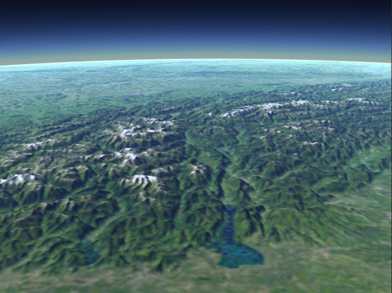
First, we discuss the scattering of air molecules, de-
                                                                 scribed by the Rayleigh scattering equation:

                                                                              I p (λ , θ ) = I0 (λ )K ρ Fr (θ )/λ 4 ,              (1)

                                                                 which describes the light scattered in a sample point P,
                                       atmosphere
                                 Pc                              in dependence of λ , the wavelength of the incident light
          Pv                      sl                             at P and θ , the scattering angle between the viewer and
                     Pa                     earth
                                                                 the incident light at P. I0 stands for the incident light,
                          sv P         Pb                        ρ for the density ratio (given by ρ = exp( −h   H0 )), de-
                                                                 pending on the altitude h and scale height H0 = 7994m,
                                                                 and Fr for the scattering phase function, which indi-
                                                                 cates the directional characteristic of scattering (Fr =
                                                                 4 (1 + cos (θ ))).
                                                                 3          2
       Figure 1: Calculation of light reaching Pv .
                                                                    K describes the constant molecular density at sea
                                                                 level
more, additional to the sky’s color, the colors of clouds                                  2π 2 (n2 − 1)2
                                                                                     K=                   ,             (2)
and sea were discussed. Another model for rendering                                              3Ns
the sky in the daytime was proposed by Preetham 15               with Ns , the molecular number density of the standard
and Hoffman 6 , a physics based night model was de-              atmosphere and n, the index of refraction of the air.
scribed by Jensen 8 . An extension of Preethams’s model             In equation 1, the relation between the scattered light
was proposed by Nielsen 11 by considering a varying              and the wavelength of the incident light describes the
density inside the atmosphere. In 2002, Dobashi et               strong attenuation of short wavelengths. This is due to
al. 4 proposed a GPU based method to implement at-               the wavelength’s inversely behavior to the light atten-
mospheric scattering using a spherical volume render-            uation. To determine the light intensity reaching Pv in
ing. They solved the discrete form of the light scatter-         Figure 1, we have to consider two steps. First, for each
ing integral by sampling it with slices. Depending on            point P between Pa and Pb , the light reaching this point
the shape of the slices, which are planar or spherical,          needs to be attenuated. Second, the resulting light in-
atmospheric scattering effects as well as shafts of light,       tensity on each point P needs to be attenuated a second
as occurring between clouds can be visualized. Later,            time on its way to the viewer at Pv . The attenuation be-
in 2004, O’Neil 13 proposed an interactive CPU imple-            tween two points inside the atmosphere is determined
mentation, solving the scattering integral by ray cast-          by the optical length, which is computed by integrat-
ing. This method avoids expensive volume rendering               ing the attenuation coefficient standing for the extinc-
by representing the atmosphere by only two spheres,              tion ratio per unit length, along the distance sv . The
one for the outer and one the inner boundary of the at-          attenuation coefficient β is given by:
mosphere. Ray casting is used to solve the discrete form
of the scattering integral by separating the ray into seg-                                  8π 3 (n2 − 1)2  4π K
                                                                                  β=                       = 4 ,                   (3)
ments and calculate the attenuation of the light and to                                         3Ns λ 4      λ
the viewer for each sample point. As the connection be-
tween the vertices of the two spheres and the viewer is          which is integrated along the distance S and yields
used as view ray, this approach strongly depends on the                           Z S
                                                                                                      4π K
                                                                                                               Z S
complexity of the scene. A vertex shader implementa-                 t(S, λ ) =         β (s)ρ (s)ds = 4             ρ (s)ds.      (4)
                                                                                   0                   λ         0
tion was published by O’Neil 14 .
   One of the main topics in terrain visualization con-          The scattering of aerosols is described with a differ-
sists of the application of continuous level of detail           ent phase function. Therefor, the improved Henyey-
methods 5;9;16 . Cignoni et al. 1 as well as Röttger et al. 17   Greenstein function by Cornette 3 is used. To adjust
used a quadtree based approach to achieve an adaptive            the rate of decrease of the aerosol’s density ratio, the
mesh refinement of the terrain data. An adaption of the          scale height H0 has to be 1.2km 19 . The optical length
BDAM approach for the application of planetary height            of aerosols is the same as for air molecules, except for
fields was published by Cignioni 2 . In our approach,            the λ14 dependance. According to Nishita 12 , if the equa-
the method of Roettger is extended for planetary terrain         tions above are applied to Equation 1, the light intensity
rendering.                                                       at Pv leads to:
                                                                                              KFr (θ )
3    ATMOSPHERIC SCATTERING                                         Iv (λ ) = Is (λ )                  ·                           (5)
                                                                                               λ4
                                                                                   Z Pb
In this section, the basic equations of Rayleigh and                                        ρ exp(−t(PPc , λ ) − t(PPa , λ ))ds.
Mie scattering are considered (according to Nishita 12 ).                              Pa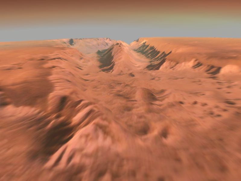
4     REAL-TIME ATMOSPHERIC SCAT-                                The algorithm works as follows: first, we define the
      TERING                                                  parametrization of our 3D texture. As discussed above,
                                                              we have to consider a number of parameters, which
In current approaches for computing atmospheric scat-
                                                              have to be reformulated in a way they can be used to
tering effects, the performance mainly depends on the
                                                              parameterize a three dimensional lookup table. For the
complexity of the scene. Therefor, the scattering in-
                                                              sake of simplicity, we now assume the observer to be
tegral of Equation 5 is solved for each vertex belong-
                                                              situated inside the atmosphere, and discuss the general
ing to the scene geometry. By applying modern graph-
                                                              case later in this section. Basically, the observer can
ics hardware, this approaches are quite fast, especially
                                                              be situated at an arbitrary position, looking in an ar-
when planets are restricted to simple spheres, consisting
                                                              bitrary direction at an arbitrary daytime. Considering
only of few vertices. But an increasing complexity of
                                                              the observer’s position Pv and his view direction Rv at a
the scene makes it impossible to compute the scattering
                                                              specific daytime we can assume that if Pv′ = (0, |Pv |, 0)T
integral for each vertex in real time anymore. This is
                                                              and R′v = (sin(θ ), cos(θ ), 0)T then
the case if you intend to render the structure of planets.
We avoid this lack of performance, by sourcing out the                          1                   1
scattering integral. Therefor, we pre compute the scat-         cos(θ ) =              < Pv , Rv >= ′ < Pv′ , R′v > . (6)
                                                                            |Pv ||Rv |             |Pv |
tering integral and store it in a 3D texture, and thereby,
we reduce the number of instructions which are neces-         This means, that each actual position and the corre-
sary to obtain the light attenuation value. The following     sponding view direction can be described by its height
sections describe the creation of the lookup texture and      h = |Pv | and the view angle θ . Exploiting this behav-
its use at the rendering stage.                               ior, we place the camera at each height inside the at-
                                                              mosphere to send out the view rays in each direction.
4.1    Creating the Scattering Texture                        Based on the fact, that the boundaries of the atmosphere
As we aim to pre compute the light scattering inte-           are considered as spherical, also the distance Pa Pb is the
gral, we have to reconsider Equation 5. It defines the        same for every view ray with angle θ with respect to the
light contribution reaching the observers eye, when it        current position Pv′ . While computing Pa Pb , it is quite
is placed at a position Pv and his view ray penetrates        important to test R′v for intersection with the inner and
the atmosphere from the point Pa to the point Pb . Basi-      the outer boundary sphere. We also have to consider,
cally, the light is attenuated two times, for each point on   that the pre computation regards the planet’s surface as
Pa Pb . The first time from the light source to a position    a simple sphere. How to deal with structured surfaces
P on the view ray, and the second time from P to the          is described in Section 4.2.
observer’s position Pv . In accordance with this obser-          To complete this formulation, we have to introduce
vation, the resulting light contribution depends on four      a light source to our model. As discussed above, the
variables: the observer’s position Pv , the position of the   attenuation from a light source to an arbitrary position
light source Pc and the entry and exit position of the at-    can also be described by the height of the sample point
mosphere Pa and Pb . Furthermore, approximating the           and the angle δ to the light source. For solving equation
integral as a Riemann sum requires an additional sam-         5 for a position Pv′ and a view ray R′v , the light attenua-
ple variable P. If we naively pre compute the scattering      tion t(PPc , λ ) and t(PPa , λ ) can easily be computed by
integral, we have to compute the light intensity for each     sampling along R′v and computing the values according
point in the atmosphere, looking in each direction. This      to the height of the sample point and its angle to the
means that we have to consider several distances Pa Pb .      light source. Finally, we introduce the daytime to our
And we also have to keep in mind, that all this pre com-      model, by applying the pre computation for all angles
putations have to be done for each position of the light      to the sun. Thus, the angle δ builds the third parameter
source. This would result in nine scalar values when          of the 3D texture.
the distance Pa Pb is represented by a three dimensional         Special consideration should be taken for the case,
vector.                                                       when the observer is situated outside the atmosphere.
   O’Neil 13 suggested to simplify the computation of         Since there is no light scattering outside the planet’s
the optical depth (Eq. 4) from the light source to P by       atmosphere, the distance of the observer to the planet
parameterizing each point P by its height and its angle       is not accounted in our pre computation step. Never-
to the Sun. This simplifies Equation 5 enormously, be-        theless, viewing the planet from outside builds a spe-
cause the pre computed values can be used to determine        cial case, in which the computation can be considered
the optical depth from the light source to the sample         the same for each position, even if the camera is sit-
point t(PPc , λ ) as well as for the attenuation from the     uated on the atmosphere’s outer boundary or the cam-
sample point to the observer. Nevertheless, the integral      era is far away. Thus, the camera has to be virtually
from Pv to P remains. For dealing with this expensive         moved towards the planet, until it hits the outer bound-
computation, we have extended O’Neils approach by             ary of the atmosphere. Afterwards, we start the compu-
additionally considering the view direction.                  tation. Thus, we only need to consider one additional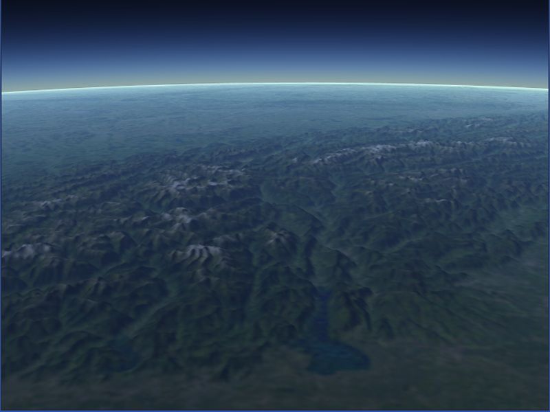
height in our pre computation: the height if the cam-
era is outside the atmosphere, which the height of the                             PV
atmosphere plus an additional, minimal offset.
      // Loop over all view angles to the                                                     Pg
            camera
  1   foreach angleViewer < resZ do
          // Get angle θ
  2       θ = GetViewAngle(angleViewer);
                                                                                                                        Pb
          // Generate a view vector                                    Figure 2: Obtaining the wrong light intensity: instead
  3       R′v = vec3d(sin(θ ), cos(θ ), 0);
                                                                       of Pg Pv the distance Pv Pb was used for the pre compu-
          // Loop over all view angles to the
                                                                       tation
                  light source
  4         foreach angleSun < resY do
                // Get angle δ
  5             δ = GetLightAngle(angleSun);                           boundary of the atmosphere. Furthermore, we enable
                // Loop over all heights of the                        front face culling to ensure, that the ray between the
                        camera                                         observer and the sphere is penetrating the atmosphere
  6               foreach height < resX do                             before the intersection. In contrast to the atmosphere,
                      // Get current height inside                     the terrain is rendered with back face culling enabled,
                            the atmosphere                             because we are only interested in the visible part of
  7                     h = f RadIn + (( f RadOut − f RadIn) ·         the planet’s surface. To obtain the light contribution,
                        height)/(resX − 1);                            first the view ray Rv = Pg − Pv is computed, where
                        // Generate the position                       Pg stands for the position of the current vertex. If
                            vector
                                                                       the observer is outside the atmosphere, the camera is
  8                     Pv = vec3d(0, h, 0);
                                                                       moved to the outer boundary. Then, the height is ob-
                        // Finally, compute the light
                            scattering
                                                                       tained by h = |Pv | as well as the cosine of the view
  9                     color = ComputeScattering(Pv , δ , Rv );       angle cos(θ ) = |Pv ||R
                                                                                             1
                                                                                               v|
                                                                                                  < Rv , Pv > and the sun angle
 10               end                                                  cos(δ ) =< Pc , Pv >. After rescaling this three param-
 11         end                                                        eters to [0, 1], the lookup texture is fetched. Because
 12   end                                                              of the nonlinear behavior of the scattering function, it
                                                                       makes sense to implement the texture fetch as a frag-
The code sample above shows how simple the 3D
                                                                       ment program, instead of a vertex program, with trilin-
lookup texture is created. The texture is given with
                                                                       ear interpolation enabled. This minimizes the interpo-
its sizes in the x, y, and z direction. For each voxel,
                                                                       lation error, since the sample frequency of the fragment
the corresponding angles and the height is used for
                                                                       shader is much higher and much faster than a compara-
computing the light intensity, by evaluating the light
                                                                       ble vertex shader implementation.
scattering integral. Therefor, we solve the discrete
form of Equation 5:                                                       In contrast to the sky, the computation of the terrain
                                                                       needs some more consideration. If we simply apply the
                              KFr (θ ) k                               texture lookup to any other vertices of the scene geom-
      Iv (λ ) = Is (λ )
                               λ 4 i=0∑ ρ exp(−tl − tv )       . (7)   etry, like the vertices representing the terrain, the com-
                                                                       putation fails. Figure 2 shows this case. This behav-
Due to the fact that the whole scattering integral is pre              ior results from the pre computation, which treats the
comuted, the sample rate k as well as the sample rate                  ray to intersect a simple sphere without considering the
for the optical depth tl and tv can be set very high.                  height field of the terrain. Thus, the light scattering is
                                                                       computed for the whole distance Pv Pb . To discuss how
4.2     Applying the Scattering Texture                                it is possible to compute the light scattering along the
                                                                       distance Pg Pv , the pre computed values have to be an-
Since the lookup texture is computed, the calculation of               alyzed. The pre computed light scattering along Pv Pb
the light intensity is quite simple and needs only few in-             can be formulated as the scattering along Pg Pv plus the
structions on the GPU. During the rendering phase, two                 scattering along Pg Pb . Rewriting Equation 5 to obtain
independent scene objects are drawn: a sphere, repre-                  the light scattering along Pg Pv would lead to
senting the sky and the planet’s surface. In Section 5,
the rendering of the terrain is discussed in more detail.
To demonstrate how the light intensity influences our                                         KFr (θ )
                                                                           Iv′ (λ ) = Is (λ )          ·                           (8)
scene, we first consider the rendering of the sky.
                                                                           Z P                λ4
                                                                                                              Pb

   Actually, the sky is represented by rendering only                              b
                                                                                                          Z
                                                                                     ρ exp(−tl − tv )ds −        ρ exp(−tl − tv )ds ,
one tesselated sphere, which is placed nearby the outer                       Pv                          Pg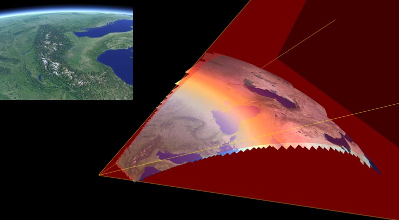
where both terms can be obtained fetching the pre com-                light attenuation between the light and the geometry can
puted texture. In fact, the first term is obtained any-               fetched as well as the attenuation between the geome-
way, simply using the current parameters as input. The                try and the observer. For the other parameters shader
second light contribution can be determined easily by                 constants are used, excepting the phase function Fr (θ )
moving the camera to the intersection point Pg without                which is pre computed as 1D texture. The follow-
changing the view angle. Then we access the lookup                    ing pseudo fragment shader code demonstrates the low
texture a second time and subtract the result from the                number of instructions used for this complex computa-
color value of the first texture lookup. By using this                tion.
mechanism, it is possible to obtain the light contribution
                                                                            // Compute Rv
for any point inside the atmosphere considering several                 1   Rv = normalize(Pg − Pv );
kinds of geometry.                                                          // If the camera is outside the
   Finally, we discuss the correct illumination of the ter-                       atmosphere, move it to the outer
rain. As we are able to compute the light scattering be-                          boundary
tween the object and the viewer, the contribution of the                2   dist = Intersect(Pv , Rv , SphereOut));
illuminated terrain has been not considered yet. Similar                3   if dist > 0 then
to the air molecules and aerosols, the light illuminat-                 4        Pv = Pv + Rv · dist;
ing the terrain is attenuated two times. While the atten-               5   end
uation from the light source to the terrain is even the                     // Compute h, θ and δ
same, the spectral shift of the illuminated terrain to the              6   h = MapToUnit(|Pv |);
                                                                        7   θ = MapToUnit(< Pv , Rv >);
observer needs to be discussed in more detail: first, we
                                                                        8   δ = MapToUnit(< Pc , Pv >);
only consider the light intensity Ig reaching the terrain                   // Get the light intensity without
geometry. Mathematically it is defined as                                         considering the height field
                                                                            Iv = tex3D(texPre3D, vec3d(h, δ , θ ));
                        KFr (θ )                                        9
    Ig (λ ) = Is (λ )            · ρ exp(−t(Pg Pc , λ )) .     (9)          // Move the camera to the intersection
                         λ4                                                       point to obtain the offset
The resulting Ig is used as incident light intensity for               10   h′ = MapToUnit(|Pg |);
illuminating the terrain geometry. We have applied a                   11   δ ′ = MapToUnit(< Pc , Pg >);
Lambert reflection, which considers the cosine of the                  12   Io f f = tex3D(texPre3D, vec3d(h′ , δ ′ , θ ));
                                                                            // Correct the intensity
angle ϕ between the incident light and the terrain nor-
                                                                       13   Iv′ = Iv − Io f f ;
mal as the intensity of the light absorbed by the terrain.                  // Now compute the light contribution
Introducing the diffuse reflection to equation 9 yields                           of the terrain
                                                                            Fr = tex1D(texPhase, θ );
                    KFr (θ )                                           14
Ig (λ ) = Is (λ )            · ρ cos(ϕ ) exp(−t(Pg Pc , λ )) . (10)    15   tgc = tex2D(texPre2D, h′ , δ ′ );
                     λ4                                                16   tgv = tex2D(texPre2D, h′ , MapToUnit(< Pg , Rv >));
Additionally, the attenuation of the reflected color                   17   Igv = Is KFr 1/λ 4 · ρ · < Ng , Pc > ·exp(−tgc − tgv );
needs to be attenuated on its way to the viewer. As de-                     // Finally, get the overall light
fined by Nishita 12 , the attenuation has to be multiplied                        intensity at Pv
with the intensity of the terrain geometry                             18   Iv′′ = Igv + Iv′ ;
                                                                       19   return Iv′′ ;
            Igv (λ ) = Ig exp(−t(Pg Pv , λ )) .              (11)     Please keep in mind, that in the case the camera is sit-
                                                                      uated inside the atmosphere, the computation of tgv re-
This equation describes the light contribution of the ter-
                                                                      quires one additional lookup (see O’Neil 13 ).
rain, without considering the light scattering along the
distance Pg Pv . Since the light contributions of all sam-
ple points are accumulated to determine the intensity
reaching the observer, Equation 8 has to be accounted                 5 PLANETARY TERRAIN RENDER-
as                                                                      ING
                       Iv′′ (λ ) = Igv + Iv′ ,               (12)
                                                                      In this section we discuss the terrain renderer we have
where Iv′′ stands for the overall intensity reaching the              optimized for the visualization of round shapes, like
observer’s eye if he is looking on the rough surface                  planets. Therefor, we extended an existing planar ter-
of a planet. While Equation 8 is implemented as two                   rain renderer 17 to render spherical objects. Indeed, the
fetches of the pre computed 3D texture, the easiest way               extension to achieve the round shape of a planet is quite
to obtain Ig and Igv , is to adopt the 2D lookup texture              easy, simply applying a spherical mapping of the ver-
described in O’Neil 13 . As this texture stores the op-               tices. However, this modification implicates a number
tical depth for each point inside the atmosphere, the                 of further necessary adaptations.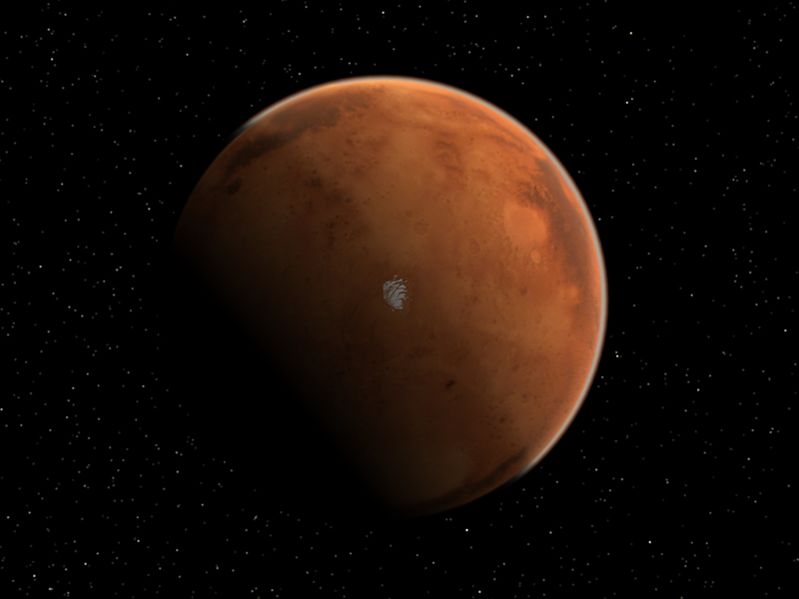
Earth Dataset     Mars Dataset
                                                                   domain size     2572 ×24×12       652 ×24×12
                                                                   outside             67.26             83.51
                                                                   inside              30.31             56.02
                                                                   only terrain
                                                                   outside             76.44            102.37
                                                                   inside              35.83            61.19

                                                              Table 1: Performance outside and inside the atmo-
Figure 3: A two stage clipping algorithm is applied on        sphere (in fps).
the whole planet. Upper left: the corresponding image
reaching the observer.
                                                                   Resolution       Optimized      Vertex Shader
 One adaption consists of the dynamic mesh refine-                     1282           608.49           151.06
ment (geomorphing). As defined in 17 , the mesh refine-                2562           181.54            35.92
ment criterion f is defined by:                                        5122            48.67             9.97
                              l
                f=                         ,          (13)    Table 2: Performance of the atmosphere only, (in fps).
                     d ·C · max(c · d2, 1)
where l is the distance to the viewer and d is the length     quad is clipped, by removing the entry of the quad tree.
of the block, which needs to be refined. The constant         Figure 3 shows the two-stage clipping (center) and the
values C and c are standing for minimum global res-           resulting visualization (upper left).
olution and the desired global resolution. The surface
roughness value is defined as d2 = d1 max |dhi |, where
dhi is the elevation difference between two refinement
                                                              6 RESULTS
levels. If f < l, the mesh needs to be refined. Applying      Table 1 shows the measured performance in frames per
this criterion to a spherical terrain representation, the     seconds. All the measurements are made on an AMD
viewpoint and the vertices needs to be in the same coor-      Athlon64 X2 Dualcore 4800+ 2.4 GHz machine with a
dinate system. To obtain a correct length l, the spherical    GeForce 7900 GT graphics card with 256 MB of mem-
transformation of the terrain needs to be attended (see       ory and a viewport of 800 × 600. First, the planets
Figure 4(i)). Therefore, if we assume the position Pv         are viewed from "outside" the atmosphere, as in Fig-
of the viewer given in world space, an inverse spherical      ure 4(a) and (g). The "inside" measurement considers
mapping of Pv is necessary.                                   the frames per second when the camera is situated in-
   For further optimization, we introduced a spherical        side the atmosphere, like in Figure 4 (c) and (h). Both
view frustum clipping: the terrain consists of several        data sets are divided into 24 tiles with respect to the
tiles, which can differ in the resolution of their local      longitude and 12 tiles with respect to the latitude. The
height field, but not in their size in world space. Thus,     quadratic value stands for the size of the tile. The reso-
a tile with a higher local resolution implicates a higher     lution of the pre computed 3D texture was chosen with
level of refinement in world space. Due to their con-         1283 . This size can be considered as sufficient. Further-
stant size, these tiles are well suited as input for the      more, it is noticeable, that larger sizes of this texture
clipping algorithm. The clipping algorithm consists of        are not really influencing the performance. If we con-
two stages: in the first stage, all non-visible tiles are     sider the measurements of Table 1, we can see that the
clipped. This stage is accomplished before the mesh           rendering outside the atmosphere is much faster than
refinement, by a comparison of the vector of the view         inside. This is due to the adaptive refinement of the ter-
direction and the four vertices, building the border of       rain mesh, which is inactive, when the observer’s dis-
the tile to be tested. If the cosine between this vectors     tance to the planet is too large. In this case, only a tes-
is negative, the tile can be considered as visible. Thus,     selated sphere is rendered. In contrast to this case, the
the first stage can be considered like a kind of crude        number of triangles increases extremely if the camera is
back face culling, just working with whole terrain tiles.     situated nearby the planet’s surface. In order to demon-
The second stage implements a smoother clipping, tak-         strate that the resulting frames per second strongly de-
ing into account the grid refinement. Therefor, the quad      pends on the performance of the terrain renderer, we re-
tree (for further information see 17 ), in which the geom-    placed the 10 tiles representing the focused mountains,
etry is stored, is traversed down and each vertex, situ-      with high resolution height fields of 1800 × 1800 cells.
ated in the center of the current quad, is tested against     This allows us to increase the number of drawn trian-
the four clipping planes. If the visibility test fails, the   gles to compare it with the achieved rendering speed, if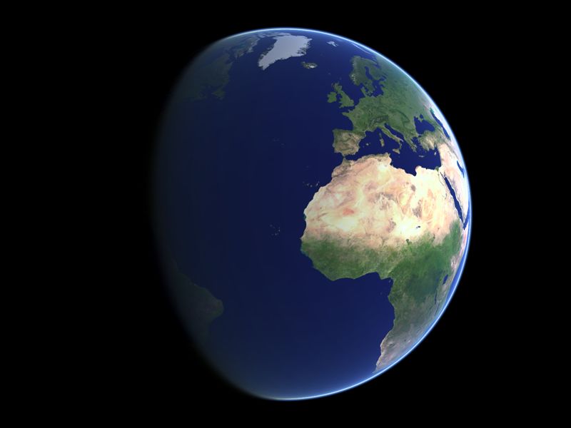
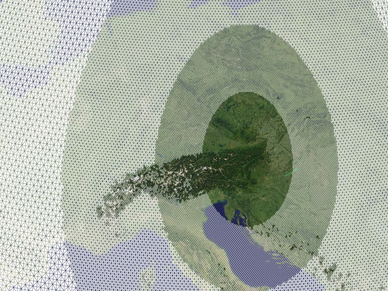
(a)                                         (b)                                       (c)

                  (d)                                         (e)                                        (f)

                  (g)                                         (h)                                        (i)
Figure 4: (a) the Earth viewed from space, (b) South America after the sunrise, (c) sunrise over the Alps, (d)
sunrise (e) early morning, (f) midday, (g) Mars viewed from space, (h) Valles Marineris with martian atmosphere,
(i) adaptive mesh refinement

only the terrain is rendered without any atmospheric ef-            simply modifying the molecular density and the wave-
fects. The mean value of the rendering power, required              length of the incident light. Additional dust particles,
for the atmospheric scattering effects, is about 15%.               which mainly influences the color of the Martian atmo-
                                                                    sphere, are unaccounted. Figure 4 (d), (e) and (f) show
   Table 2 shows the increase in performance, when the
                                                                    the Alps viewed from Italy at different day times, start-
evaluation of the scattering integral is optimized by our
                                                                    ing with the sunrise, over to the early morning hours
method. The frames per second of our implementation
                                                                    to midday. This sequence illustrates the dependency of
are compared with a vertex shader implementation. For
                                                                    the light scattering and the angle to the sun. Finally, (i)
this measurements, only the atmosphere is rendered ap-
                                                                    demonstrates how our spherical refinement mechanism
plying 2 spheres with the given number of vertices per
                                                                    works.
sphere. The resolution of the pre computed 3D texture
is also 1283 . The table shows, that our method is 4 - 5.3
times faster than the vertex shader implementation. It is           7 CONCLUSION AND FUTURE
also perceptible, that this ratio increases proportional to           WORK
the number of rendered triangles, what can be ascribed
                                                                    We have presented an interactive technique for plane-
to the high number of vertex shader instructions and the
                                                                    tary rendering taking into account atmospheric scatter-
costs of vertex texture fetches.
                                                                    ing effects. High efficiency is achieved by combining
  Figure 4 (g) and (h) demonstrate the flexibility of               the CPU based terrain renderer with the atmospheric
the applied light scattering method, by replacing the               rendering. Therefor, the complete scattering integral,
Earth’s atmosphere with the Martian atmosphere by                   described by Nishita 12 , is evaluated in a separate pre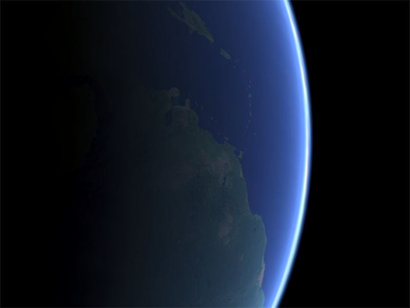
computation step. This is done by computing the at-          [7] H.W. Jensen and P.H. Christensen. Efficient sim-
mospheric scattering for each position inside the atmo-          ulation of light transport in scences with partici-
sphere, parameterized by its height and the angles to the        pating media using photon maps. In SIGGRAPH
                                                                 ’98: Proceedings of the 25th annual conference
viewer and to the Sun. The results are stored into one           on Computer graphics and interactive techniques,
3D texture. The GPU is used to compute the light in-             pages 311–320, 1998.
tensity reaching the observer’s eye, regarding the struc-
ture of the planet’s surface and the correct illumination    [8] H.W. Jensen, F. Durand, J. Dorsey, M.M. Stark,
                                                                 P. Shirley, and S. Premoze. A physically-based
of the terrain geometry. We have discussed, how the              night sky model. In SIGGRAPH ’01: Proceed-
pre computed 3D texture can be used to solve the prob-           ings of the 28th annual conference on Computer
lems mentioned above. Finally, a planetary terrain ren-          graphics and interactive techniques, pages 399–
derer was introduced for the adaptive mesh generation            408, 2001.
and rendering of height fields on spherical objects. The     [9] P. Lindstrom, D. Koller, W. Ribarsky, L. F.
results shows clearly, that the evaluation of the scatter-       Hodges, N. Faust, and G.A. Turner. Real-time,
ing integral is absolutely independent of the scene com-         continuous level of detail rendering of height
plexity, what makes it attractive to utilize it with large       fields. In SIGGRAPH ’96: Proceedings of the
scale renderings.                                                23rd annual conference on Computer graphics
                                                                 and interactive techniques, pages 109–118, 1996.
   In the future, the 3D texture can also be used for
rendering other scenes, like snow or rain simulations. It    [10] N.L. Max. Atmospheric illumination and shad-
is also thinkable to use it as part of a complete weather         ows. In SIGGRAPH ’86: Proceedings of the 13th
simulation or to illuminate large outdoor scenes in               annual conference on Computer graphics and in-
                                                                  teractive techniques, pages 117–124, 1986.
games.
                                                             [11] R.S. Nielsen. Real time rendering of atmospheric
                                                                  scattering effects for flight simulators. Master’s
8   ACKNOWLEDGMENTS                                               thesis, Informatics and Mathematical Modelling,
We would like to thank the NASA for providing the                 Technical University of Denmark, DTU, 2003.
earth textures and the MOLA datasets of Earth and            [12] T. Nishita, T. Sirai, K. Tadamura, and E. Naka-
Mars.                                                             mae. Display of the earth taking into account at-
                                                                  mospheric scattering. In SIGGRAPH ’93: Pro-
                                                                  ceedings of the 20th annual conference on Com-
REFERENCES                                                        puter graphics and interactive techniques, pages
[1] P. Cignoni, F. Ganovelli, E. Gobbetti, F. Marton,             175–182, 1993.
    F. Ponchio, and R. Scopigno. BDAM – batched
    dynamic adaptive meshes for high performance             [13] S. O’Neal. Real-time atmospheric scattering.
    terrain visualization. Computer Graphics Forum,               www.gamedev.net/reference/articles/article2093.asp,
    22(2):505–514, 2003.                                          2004.
                                                             [14] S. O’Neal. Accurate atmospheric scattering. GPU
[2] P. Cignoni, F. Ganovelli, E. Gobbetti, F. Marton,             Gems, 2:253–268, 2005.
    F. Ponchio, and R. Scopigno. Planet-sized batched
    dynamic adaptive meshes (P-BDAM). In Proc.               [15] A.J. Preetham, P. Shirley, and B. Smits. A prac-
    IEEE Visualization, pages 147–155, 2003.                      tical analytic model for daylight. In SIGGRAPH
                                                                  ’99: Proceedings of the 26th annual conference
[3] W.M. Cornette and J.G. Shanks. Physical reason-               on Computer graphics and interactive techniques,
    able analytic expression for the single-scattering            pages 91–100, 1999.
    phase function. Applied Optics, 31(16):3152–
    3160, 1992.                                              [16] E. Puppo. Variable resolution terrain surfaces. In
                                                                  Proceedings of the 8th Canadian Conference on
[4] Y. Dobashi, T. Yamamoto, and T. Nishita. Inter-               Computational Geometry, pages 202–210, 1996.
    active rendering of atmospheric scattering effects
    using graphics hardware. In HWWS ’02: Proceed-           [17] S. Röttger, W. Heidrich, P. Slusallek, and H.-P.
    ings of the ACM SIGGRAPH/EUROGRAPHICS                         Seidel. Real-time generation of continuous lev-
    conference on Graphics hardware, pages 99–107,                els of detail for height fields. In Proc. WSCG ’98,
    2002.                                                         pages 315–322, 1998.
                                                             [18] H.E. Rushmeier and K.E. Torrance. The zonal
[5] M.H. Gross, R. Gatti, and O. Staadt. Fast multires-           method for calculating light intensities in the pres-
    olution surface meshing. In VIS ’95: Proceedings              ence of a participating medium. In SIGGRAPH
    of the 6th conference on Visualization ’95, page              ’87: Proceedings of the 14th annual conference
    135, 1995.                                                    on Computer graphics and interactive techniques,
                                                                  pages 293–302, 1987.
[6] N. Hoffman and A.J. Preetham.          Real-time
    light-atmosphere interactions for outdoor scenes.        [19] S. Sekine. Optical characteristics of turbid atmo-
    Graphics programming methods, pages 337–352,                  sphere. J Illum Eng Int Jpn, 71(6):333, 1992.
    2003.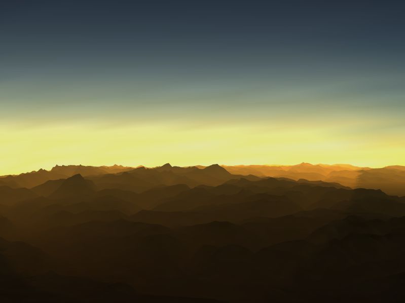
You can also read