Dense Semi-Rigid Scene Flow Estimation from RGBD images
←
→
Page content transcription
If your browser does not render page correctly, please read the page content below

Dense Semi-Rigid Scene Flow Estimation from
                  RGBD images ⋆

    Julian Quiroga1,3, Thomas Brox2 , Frédéric Devernay1 , and James Crowley1
                         1
                         PRIMA team, INRIA Grenoble, France
                            firstname.lastname@inria.fr
           2
             Department of Computer Science, University of Freiburg, Germany
                              brox@cs.uni-freiburg.de
      3
          Departamento de Electrónica, Pontificia Universidad Javeriana, Colombia
                            quiroga.j@javeriana.edu.co

          Abstract. Scene flow is defined as the motion field in 3D space, and
          can be computed from a single view when using an RGBD sensor. We
          propose a new scene flow approach that exploits the local and piece-
          wise rigidity of real world scenes. By modeling the motion as a field of
          twists, our method encourages piecewise smooth solutions of rigid body
          motions. We give a general formulation to solve for local and global rigid
          motions by jointly using intensity and depth data. In order to deal effi-
          ciently with a moving camera, we model the motion as a rigid component
          plus a non-rigid residual and propose an alternating solver. The evalu-
          ation demonstrates that the proposed method achieves the best results
          in the most commonly used scene flow benchmark. Through additional
          experiments we indicate the general applicability of our approach in a
          variety of different scenarios.

          Keywords: motion, scene flow, RGBD image

1     Introduction

The 3D motion field of a scene is useful for several computer vision applications,
such as action recognition, interaction, or 3D modeling on nonrigid objects. One
group of methods uses a stereo or multi-view camera system, where both scene
flow and depth are estimated from the images, while a second group uses RGBD
images as input. In the latter case, the depth given by the sensor may be used
directly for scene flow estimation. In this paper, we present a new formulation
for this second group.
    The two main questions for scene flow estimation from RGBD images are:
(a) how to fully exploit both sources of data, and (b) which motion model should
be used to compute a confident scene flow. When both intensity and depth are
⋆
    This work was supported by a collaborative research program between Inria Grenoble
    and University of Freiburg. We gratefully acknowledge partial funding by CMIRA
    2013 (Region Rhône-Alpes), GDR ISIS (CNRS), and COLCIENCIAS (Colombia).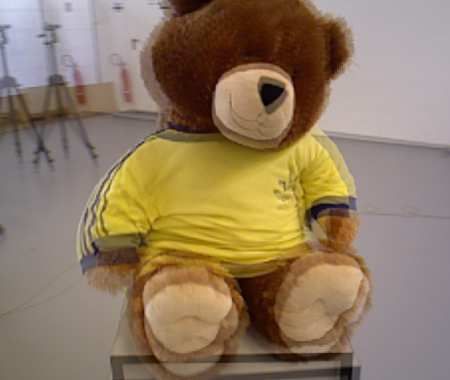
2      J. Quiroga, T. Brox, F. Devernay, J. Crowley

provided, there is not a consensus on how to combine these two sources of infor-
mation most effectively. A straightforward approach would compute the optical
flow from RGB images and infer the scene flow from the depth data. It is also
possible to generate colored 3D point clouds and try to find out the 3D motion
vectors consistent with the input data. However, it is not mandatory to explicitly
represents points in 3D to solve for the scene flow: the scene structure can be
represented in the image domain, where color and depth data can be coupled
using a projective function. This way, depth changes influence the motion in the
image domain and consistency constraints can be formulated jointly over the
color and depth images. This is the approach we follow in this work. It gives us
access to some of the powerful tools developed for 2D motion estimation.
    The second question has been addressed less. Scene flow estimation using in-
tensity and depth is an ill-posed problem and regularization is needed. Usually,
the 3D motion vector of each point is solved to minimize color and intensity
constraints in a data term and the whole 3D motion field is regularized to get
spatially smooth solutions while preserving discontinuities. Since depth data is
available, a weighted regularization can be used to preserve motion disconti-
nuities along depth edges, where independent motions are probable to appear.
However, solving for a piecewise smooth solution of the 3D motion field may
not be the best choice for some motions of interest. For example, a 3D rotation
of a rigid surface induces a great variety of 3D motions that are hardly well
regularized by such an approach. A similar issue occurs when the RGBD sensor
is moving with respect to the scene.
    In this work, we take advantage of the fact that most real scenes can be well
modeled as locally or piecewise rigid, i.e., the scene is composed of 3D indepen-
dently rigid components. The main contribution of this paper is the definition of
an over-parametrized framework for scene flow estimation from RGBD images.
We model the scene flow as a vector field of rigid body motions. This repre-
sentation helps the regularization process which, instead of directly penalizing
variations in the 3D motion field, encourages piecewise smooth solutions of rigid
motions. Moreover, the proposed rigid body approach can be constrained in the
image domain to fully exploit intensity and depth data. This formulation is flex-
ible enough to support different data constraints and regularization strategies,
and it can be adapted to more specialized problems. By using the same general
framework, it is possible to model the scene flow as a global rigid motion plus
a non-rigid residual, which is particularly useful when estimating the motion of
deformable objects in conjunction with a moving camera.

2   Related work

Scene flow was first introduced by Vedula [18] as the 3D motion field of the
scene. Since this seminal work several approaches have been proposed to compute
the 3D motion field. If a stereo or multi-view camera system is available, the
scene flow can be computed by enforcing consistency with the observed optical
flows [18], by a decoupled [21] or joint [1, 8] estimation of structure and motion,
Dense Semi-Rigid Scene Flow Estimation from RGBD images             3

or by assuming a local rigidity of the scene [19]. In this work we assume that
a depth sensor is available and the estimation of the structure is not needed.
The first work using intensity and depth was by Spies et al. [16], where the
optical flow formulation by Horn and Schunck [7] is extended to include depth
data. In this approach, depth data is used simply as an additional channel in the
variational formulation of the optical flow. The range flow is estimated using the
observed data and enforced to be smooth. However, the scene is assumed to be
captured by an orthographic camera and there is no coupling between optical
and range flows. The coupling issue can be solved as in [10], where the scene
flow is directly solved using the depth data to constrain the 3D motion in the
image domain. However in that work, the depth data is not fully exploited since
there is no range flow constraint. Similar to [16], this method suffers from the
early linearization of the constancy constraints and from over-smoothing along
motion boundaries because of the L2 -regularization. Quiroga et al. [12] define
a 2D warping function to couple image motion and 3D motion, allowing for a
joint local constraint of the scene flow on intensity and depth data. Although the
method is able to deal with large displacements, it fails on untextured regions
and more complex motions, such as rotations.
    In order to solve for dense scene flow, a regularization procedure is required.
Usually, the 3D motion field is assumed to be piecewise smooth, and total vari-
ation (TV) is used as regularizer. The work by Herbst [6] follows this idea, but
as [16], it lacks a coupling between optical and range flows, and the regularization
is done on the optical flow rather than on the scene flow. In [13], a variational
extension of [12] is presented. A weighted TV is applied on each component of
the 3D motion field, aiming to preserve motion discontinuities along depth edges.
    All these methods assume spatial smoothness of the scene flow, which is a
reasonable assumption for translational motions but not for rotations. Under
a rotation, even close scene points present different 3D motions. In case of a
moving camera the regularization of the motion field can be a challenge. In this
work, we use an over-parametrization of the scene flow, where each scene point is
allowed to follow a rigid body motion. This way, the regularization can be done
on a field of rigid motions, favoring piecewise solutions, which is a better choice
for real scenes. A similar idea is presented in [14], where a regularization of a
field of rigid motions is proposed. Our approach differs from that work in three
ways. First, we use a more compact representation of the rigid-body motion
via the 6-parameter twist representation, instead of a R12 embedding. Second,
our approach solves and regularizes the rigid motion field at the same time.
Finally, we decouple the regularization of the rotational and translational fields,
which simplifies the optimization and allows the use of different TV strategies
on each field. Similar to [12], we use a depth-based weighting function to avoid
penalization along surface discontinuities.
    In an alternative approach, Hadfield and Bowden [5] estimate the scene flow
using particle filtering in a 3D colored point cloud representation of the scene.
In that approach, a large set of motion hypotheses must be generated and tested
for each 3D point, leading to high computational costs. We rather use the 2D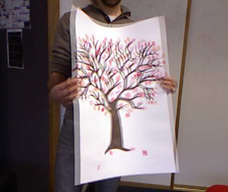
4      J. Quiroga, T. Brox, F. Devernay, J. Crowley

parametrization provided by RGBD sensors to formulate an efficient 3D motion
exploration. As done in [12], we define a warping function to couple the twist
motion and the optical flow. A very similar warp is presented in [9] to solve for
a global rigid motion from RGBD images. In our approach, we use the warping
function to locally constrain the rigid motion field in the image domain. The
global rigid motion estimation can be seen as a particular case of the proposed
formulation. Moreover, unlike [9], we define a depth consistency constraint to
fully exploit both sources of data. Thus, we can solve for the local twist motion
that best explains the observed intensity and depth data, gaining robustness un-
der noise. The local solver, in conjunction with the TV regularization of the twist
field, provides an adjustable combination between local and piecewise rigidity.
    As we present in the experiments, this framework is flexible enough to es-
timate a global rigid body motion or to solve for a general 3D motion field in
challenging setups. This way, we are able to model the motion of the scene as a
global rigid motion and a non-rigid residual.

3     Scene motion model
We parameterize every visible 3D point into the image domain Ω ⊂ R2 . The
projection π : R3 → R2 maps a 3D point X = (X, Y, Z) onto a pixel x = (x, y)
on Ω by:
                                                 T
                                 X         Y
                     π(X) = fx + cx , fy + cy        ,                  (1)
                                 Z         Z
where fx and fy are the focal lengths of the camera and (cx , cy ) its principal
point. The inverse projection π −1 : R2 × R → R3 back-projects an image point
to the 3D space for a given depth z, as follows:
                                                      T
                                     x − cx y − cy
                     π −1 (x, z) = z        ,z      ,z    .                  (2)
                                       fx        fy
We will use X or π −1 (x, z) as the 3D representation of image point x.
   The scene flow v(x) : Ω → R3 is defined as the 3D motion field describing
the motion of every visible 3D point between two time steps accordingly
                              Xt+1 = Xt + v (xt ) .                            (3)

3.1   Twist motion field
Instead of directly representing the elements of the motion field as 3D vectors,
we use an over-parametrized model to describe the motion of every point as a
rigid transformation. The group action of a rigid body transformation can be
written as T (X) = RX + t, where t ∈ R3 is a translation, and R ∈ SO(3) is
a rotation matrix. Using homogeneous coordinates, a 3D point X̃ = (X, 1)T is
transformed into X̃′ accordingly to

                    ′                         R t
                  X̃ = GX̃, with G =                 ∈ SE(3).                (4)
                                            01×3 1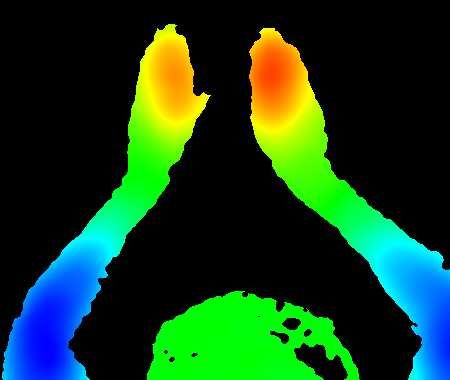
Dense Semi-Rigid Scene Flow Estimation from RGBD images 5
Since G has only 6 degrees of freedom, a more convenient and compact rep-
resentation is the 6-parameter twist. Every rigid motion can be described as a
rotation around a 3D axis ω = (ωX , ωY , ωZ )T and a translation τ = (τx , τy , τz )T
along this axis. Therefore it can be shown that for any arbitrary G ∈ SE(3)
there exists an equivalent ξ ∈ R6 twist representation. A twist ξ = (τ, ω) can be
converted into the G representation with the following exponential map:
ˆ2
(ξ) ˆ3
(ξ)
G = eξ̂ = I + ξ̂ + ++ + ··· , (5)
2! 3!
where
0 −ωZ ωY
ω̂ τ
ξ̂ = , with ω̂ = ωZ 0 −ωX . (6)
01×3 1
−ωY ωX 0
Correspondingly, for each G ∈ SE(3) there exist a twist representation given by
the logarithmic map via ξ = log(G); see [11] for more details.The motion of the
scene is embedded in a twist motion field ξ(x) : Ω → R6 , where the motion of
every 3D point between two time steps is given by:
X̃t+1 = eξ̂(xt ) X̃t . (7)
3.2 Twist motion on the image
For every time t the scene is registered as an RGBD image St (x) = {It (x), Zt (x)}
where images I(x) and Z(x) provide color and depth, respectively, for every
point x ∈ Ω. Under the action of a twist ξ between t and t + 1, the motion
of a 3D point induces an image flow (u, v). We define the warping function
W(x, ξ) : R2 ×R6 → R2 that maps each non-occluded pixel onto its new location
after the rigid motion. The warping function is defined as:
−1
π (x, Z(x))
W(x, ξ) = π eξ̂ X̃ , with X̃ = . (8)
1
Let S k (x) be a component of the RGBD image (e.g. brightness or depth) eval-
uated at x ∈ Ω and let ρS k (x, ξ) be a robust error function between Stk (x) and
k
St+1 (W(x, ξ)). Every twist motion vector ξ is solved to minimize one or sev-
eral consistency functions ρS k (x, ξ). Optimization problems on manifolds such
as SE(3) can be solved by calculating incremental steps in the tangent space
to the manifold. Considering that an initial estimate ξ is known, the goal at
each optimization step is to find the increment ∆ξ which (approximately) min-
imizes ρS k (x, ξ). Since SE(3) is a Lie group (not an Euclidean space) with
the composition as operation, the exponential and logarithmic functions are
used to update the current estimate ξ with the new increment ∆ξ according to
ˆ
ξ ← log(e∆ξ eξ̂ ) [11]. The iterative solution requires a linearization of the warping
function. Given the initial estimate ξ, the image point x becomes xξ = W(x, ξ)
and the warping function satisfies:
ˆ
W(x, log(e∆ξ eξ̂ )) = W(xξ , ∆ξ) = xξ + δx(xξ , ∆ξ), (9)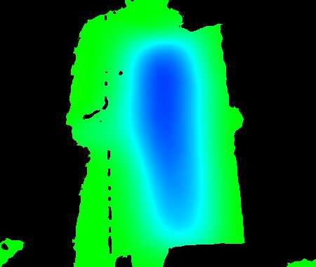
6 J. Quiroga, T. Brox, F. Devernay, J. Crowley
where δx(xξ , ∆ξ) is the image flow induced by the increment ∆ξ, which is given
ˆ T
by δx(xξ , ∆ξ) = π(e∆ξ X̃ξ ) − π(X̃ξ ), with X̃ξ = π −1 (xξ , Z(xξ )), 1 . Assuming
ˆ
a small rotation increment, the exponential function is approximated as e∆ξ ≈
ˆ Therefore for a small increment ∆ξ the warping function can be well
I + ∆ξ.
approximated by the following linear version:
ˆ
W(x, log(e∆ξ eξ̂ )) = W(x, ξ) + J(xξ )∆ξ, (10)
where J(xξ ) is the Jacobian matrix, given by:
fx x x y fx +x2ξ yξ fx
0 − Z(xξξ ) − fξy ξ −
Z(xξ ) fy fy
J(xξ ) = . (11)
fy y fy +y 2 xξ yξ xξ fy
0 Z(x ξ)
− Z(xξξ ) − fx ξ fx fx
4 Scene flow formulation
Given two pairs of RGBD images {I1 , Z1 } and {I2 , Z2 } the goal is to solve
for the scene flow field that best explains the observed data. Due to vanishing
gradients, the aperture problem and outliers, this motion computation is an ill-
posed problem that cannot be solved independently for each point. Therefore, a
smoothness in the motion field must be assumed. In our formulation, we consider
only spatial smoothness, but it can be extended to temporal smoothness. In
general, we solve for the twist field ξ minimizing the following energy:
E(ξ) = ED (ξ) + αES (ξ), (12)
where the data term ED (ξ) measures how consistent is the estimated twist-based
model with the observed color and depth data, and the smoothness term favors
piecewise smooth fields while preserving discontinuities.
4.1 Data term
The warping function (8) enables the formulation of consistency constraints for
the twist field in the image domain. Using the gray value image we define a
brightness constancy assumption:
I2 (W(x, ξ)) = I1 (x), (13)
and a gradient constancy assumption:
I2g (W(x, ξ)) = I1g (x). (14)
where I g (x) = |∇I(x)|. The gradient assumption reduces the effect of brightness
changes. We use the gradient magnitude since it is invariant to rotation. The
estimated twist motion should satisfy these constraints for most points.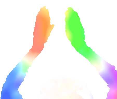
Dense Semi-Rigid Scene Flow Estimation from RGBD images                7

   On the other hand, the surface changes under the twist action. This variation
must be consistent with the observed depth data. Therefore we define a depth
variation constraint given by:
                          Z2 (W(x, ξ)) = Z1 (x) + δZ (x, ξ),                       (15)
where δZ (x, ξ) is the depth variation induced on the 3D point π −1 (x, Z1 (x)) by
the twist ξ, obtained from the third component of the 3D vector:
                                                     −1
                                                      π (x, Z1 (x))

                          ξ̂
          δ3D (x, ξ) = e − I4×4 X̃        with X̃ =                    .      (16)
                                                            1
This equation enforces the consistency between the motion captured by the
depth sensor and the estimated motion.
    Without regularization, equations (13), (14) and (15) alone are not sufficient
to constrain the twist motion for a given point since there is an infinite number
of twists that satisfy these constraints. However, real scenes are locally rigid
and it is possible to solve for a local twist explaining the observed motion. We
formulate the twist motion estimation as a local least-square problem by writing
the data term as follows:
           X X
                     Ψ ρ2I (x′ , ξ (x)) + γρ2g (x′ , ξ (x)) + λΨ ρ2Z (x′ , ξ (x)) , (17)

 ED (ξ) =
             x x′ ∈Nx

where Nx is an image neighborhood centered on x, and with the brightness,
gradient and depth residuals, respectively given by:
                   ρI (x, ξ) = I2 (W(x, ξ)) − I1 (x) ,                             (18)
                   ρg (x, ξ) = I2g (W(x, ξ)) − I1g (x) ,                           (19)
                  ρZ (x, ξ) = Z2 (W(x, ξ)) − (Z1 (x) + δZ (x, ξ)).                 (20)
Constant γ balances brightness and gradient residuals,
                                                 √ while λ weights intensity
and depth terms. We use the robust norm Ψ s2 = s2 + ε2 , which is a differ-
entiable approximation of the L1 norm, to cope with outliers due to occlusion
and non-rigid motion components in Nx .

4.2   Smoothness term
A twist motion field ξ can be decomposed into a rotational field ω, with eω̂ : Ω →
SO(3), and a 3D motion field τ : Ω → R3 . Since they are decorrelated by nature,
we regularize each field independently using weighted Total Variation (TV),
which allows piecewise smooth solutions while preserving motion discontinuities.
    Regularization of the fields ω and τ poses different challenges. Elements of
τ lie in the Euclidean space R3 and the problem corresponds to a vector-valued
function regularization. Different TV approaches can be used to regularize τ , as
described in [4]. Particularly the channel-by-channel L1 norm has been success-
fully used for optical flow [22]. We define the weighted TV of τ as:
                                      X
                           TVc (τ ) =     c(x) k∇τ (x)k ,                      (21)
                                         x
8       J. Quiroga, T. Brox, F. Devernay, J. Crowley

                                                                              2
where k∇τ k := |∇τX | + |∇τY | + |∇τZ | and c(x) = e−β|∇Z1 (x)| . The weighting
function c helps preserve motion discontinuities along edges of the 3D surface.
Moreover, the L1 norm can be replaced by the Huber norm [23] to reduce the
staircasing effect. Efficient solvers for both norms are presented in [3].
    Elements of ω are rotations in the Lie group SO(3) embedded in R3 through
the exponential map, and the regularization has to be done on this manifold.
In order to apply a TV regularization, a notion of variation should be used for
elements of SO(3). Given two points eω̂1 , eω̂2 ∈ SO(3) the residual rotation can
                   ˆ 1 ω̂2
be defined as e−ω       e . The product in logarithmic coordinates can be expressed
as eω̂1 eω̂1 = eµ(ω̂1 ,ω̂2 ) , where the mapping µ can be expanded in a Taylor series
around the identity, using the Baker-Campbell-Hausdorff formula:

                                            1
                 µ(ω̂1 , ω̂2 ) = ω̂1 + ω̂2 + [ω̂1 , ω̂2 ] + O(|(ω̂1 , ω̂2 )|3 ),   (22)
                                            2

where [·, ·] is the Lie bracket in so(3). Close to the identity, (22) is well ap-
proximated by its first-order terms, so that for small rotations the variation
measure can be defined as the matrix subtraction in so(3), or equivalently, as
a vector difference for the embedding in R3 . Accordingly, the derivative matrix
Dω := (∇ωX , ∇ωZ , ∇ωZ )T : Ω → R3×2 approximates the horizontal and verti-
cal point-wise variations of ω on the image. Following [4], we define the TV as
the sum over the largest singular value σ1 of the derivative matrix:

                                          X
                           TVσ (ω) =            c(x) σ1 (Dω(x)) .                  (23)
                                            x

This TV approach supports a common edge direction for three components,
which is a desirable properties for the regularization of the field of rotations.
Moreover, deviations are less penalized with respect to other measures (e.g.
Frobenius norm [14]) and efficient solvers are available. However, this TV defini-
tion approximates the real structure of the manifold yielding to a biased measures
far from the identity. The more the rotation is away from the identity, the more
its variations in SO(3) are penalized as is shown hereinafter. Given two rotations
         ω−1 and ω2 = θ2 ←
ω 1 = θ1 ←               ω−2 , with θ the angle and ←− the unitary axis vector of the
                                                     ω
rotation, and writing θ2 = θ1 + δθ, leads to ω2 − ω1 = θ1 (←  ω−2 − ←
                                                                    ω−1 ) − δθ←
                                                                              ω−2 . This
linearly dependent penalization usually is not a problem, since large rotations
imply larger motion on the image. Thus, a stronger regularization can be rea-
sonable. Moreover, large rotation caused by a global motion of the scene or the
camera can be optimized separately and compensated, as we show in Sec. 4.4.
Optionally, this over-penalization can be removed by expressing each rotation
as ω = θ←   − and applying a vectorial TV on ←
            ω                                      − and a scalar TV on θ. In our
                                                   ω
approach, the full smoothing term is given by:

                             ES (ξ) = TVc (τ ) + TVσ (ω).                          (24)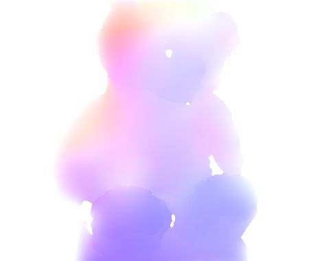
Dense Semi-Rigid Scene Flow Estimation from RGBD images                9

4.3   Optimization
The proposed energy (12) is minimized by decomposing the optimization into
two simpler problems. We use the variable splitting method [20] with auxiliary
variable χ, and the minimization problem becomes:
                                           1 X
                  min ED (ξ) +                 |ξ(x) − χ(x)|2 + αES (χ),             (25)
                   ξ,χ                    2κ x
where κ is a small numerical variable. Note that the linking term between ξ and
χ is the distance on the tangent space at the identity in SE(3). The solution of
(25) converges to that of (12) as κ → 0. Minimization of this energy is performed
by alternating the two following optimization problems:

i. For fixed χ, estimate ξ that minimizes (25). This optimization problem can
be solved point-wise by minimizing:
                    1        2
                                X
                                     Ψ ρ2I + γρ2g + λΨ ρ2Z ,

                      |ξ − χ| +                                          (26)
                   2κ           ′          x ∈Nx
                                  ′
where the parameters (x , ξ) are considered implicit. This energy can be lin-
earized around an initial estimate ξ, using a first-order Taylor series expansion:
   1                      2                                                   2

                                           Ψ |ρI + Ix J∆ξ|2 + γ |ρG + Igx J∆ξ|
                                      X
     log(e∆ξ̂ eξ̂ ) − χ       +
  2κ
                                  x′ ∈Nx

                                                                              2
                                                     + λΨ |ρZ + (Zx J − K) ∆ξ| . (27)

where Ix , Igx and Zx are the row vector gradients of I2 (x), Ig2 (x) and Z2 (x),
respectively, and J is the Jacobian (11) of the warp, all evaluated at xξ =
W(x, ξ). The 1 × 6 vector K is defined as K = D ([Xξ ]× |I3×3 ) with D = (0, 0, 1)
isolating the third component and [·]× the cross product matrix. Finding the
minimum of (27) requires an iterative approach. Taking the partial derivative
with respect to ∆ξ and setting it to zero, the increment ∆ξ can be computed as:
                 "
                   X
              −1
                        Ψ ′ ρ2I + γρ2G (Ix J)T ρI + γ(Igx J)T ρG

   ∆ξ = −H
                  x′ ∈Nx
                                                       o 1
                              +λ Ψ ′ ρ2Z (Zx J − K)T ρZ + log (eξ̂ )−1 eχ̂ , (28)

                                                         κ
where Ψ ′ is the derivative of the robust norm, which is evaluated at the current
estimate ξ. The 6 × 6 matrix H is the Gauss-Newton approximation of the
Hessian matrix and is given by:
        X                   h      T                 T
                                                               i
  H=          Ψ ′ ρ2I + γρ2G (Ix J) (Ix J) + γ (Igx J) (Igx J)
       x′ ∈Nx

                                                            T              1
                                      + λ Ψ ′ ρ2Z (Zx J − K) (Zx J − K) +

                                                                             I6×6 . (29)
                                                                          2κ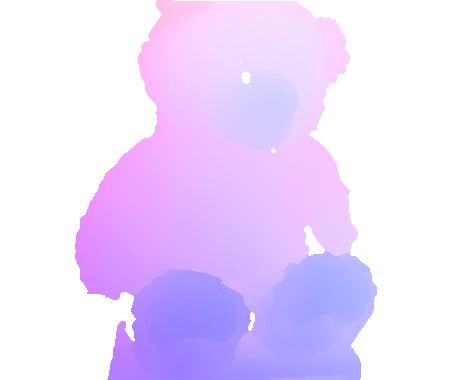
10     J. Quiroga, T. Brox, F. Devernay, J. Crowley

ii. For fixed ξ = (ω, τ ), compute χ = (̟, π) that minimizes:
  (                                 ) (                                   )
               ηX                 2                 ηX                  2
    TVc (π) +       |π(x) − τ (x)| + TVσ (̟) +            |̟(x) − ω(x)|     (30)
               2 x                                   2 x

where η = (κα)−1 . Each side of equation (30) corresponds to a vectorial image
denoising problem with a TV-L2 model (ROF model). Efficient primal-dual al-
gorithms exist for solving both problems. The left side is solved component-wise
using the first-order primal-dual algorithm [3]. For the right side we use the
vectorial approach [4] which allows an optimal coupling between components. A
small modification is necessary in both cases to include the weighting function.

4.4   Scene flow with camera motion estimation
In many applications, the sensor itself moves relative to the observed scene and
causes a dominant global motion in the overall motion field. In this situation,
compensating for the motion of the camera can simplify the estimation and
regularization of the scene flow. Moreover, for 3D reconstruction of deformable
objects, the camera motion is needed to register partial 3D reconstructions.
Therefore, we consider splitting the motion of the scene into a globally rigid
component ξR = (τR , ωR ) ∈ R6 , capturing the camera motion relative to the
dominant object/background, plus a non-rigid residual field ξ = (τ, ω). We as-
sume that a large part of the scene follows the same rigid motion. Accordingly,
the scene flow is defined as the composition χ = log(eξ̂ + eξ̂R − I4×4 ), and the
estimation problem is formulated as:

                             min ERig (χ) + ERes (χ) ,                      (31)
                               χ

with ERig (χ) and ERes (χ) the rigid and non-rigid energies, respectively. It is
worth noting that the separation of the camera motion is in addition to the
framework presented above, i.e., the non-rigid part can still deal with local mo-
tion.

Rigid energy. The camera motion can be estimated using the data term (17),
by considering every pixel (or a subset of Ω) to solve for a unique twist ξR .
Accordingly, the rigid component of the energy is defined as:
                       X
                          Ψ ρ2I (x, χ) + γρ2g (x, χ) + λΨ ρ2Z (x, χ) .

          ERig (χ) =                                                     (32)
                        x

Non-rigid residual energy. The residual motion can be computed following
(12), with the non-rigid energy given by:

                            ERes (χ) = ED (χ) + αES (χ).                    (33)

We minimize (31) by an iterative, alternating estimation of ξR and ξ:
Dense Semi-Rigid Scene Flow Estimation from RGBD images 11
a. Given a fixed ξ, solve for ξR that minimizes ERig (χ). This is done by itera-
tively applying (28) and (29), with a zero auxiliary flow.
b. Given a fixed ξR , solve for ξ that minimizes ERes (χ). This is done by iterating
steps i and ii in Sec. 4.3.
5 Experiments
5.1 Implementation details
In order to compute the scene flow, the proposed method assumes that a pair of
calibrated RGBD images is provided. Regardless of the depth sensor, depth data
is always processed in cm and RGB color images are transformed to intensity
images and normalized. For all the experiments α = 10, β = 1, γ = 0.1 and
λ = 0.1. For each scene a depth range is defined and only pixels having a valid
depth measure inside the range are taken into account for the data term and
final measurements. However, all pixels are considered in the regularization.
We use a multi-scale strategy in order to deal with larger motions. We con-
struct an image pyramid with a downsampling factor of 2. We apply a Gaussian
anti-aliasing filter to the intensity image and the pyramid is built using bicubic
downsampling. For the depth image, a 5 × 5 median filter is used and the pyra-
mid is constructed by averaging pixels in non-overlapped neighborhoods of 2 × 2,
where only pixels with a valid depth measure are used. Having a pyramid with
levels l = {0, 1, ..., L}, with 0 the original resolution, the computation is started
at level L an the estimated twist field is directly propagated to the next lower
level. The camera matrix is scaled at each level by the factor 2l . The neighbor-
hood Nx is defined as a N × N centering window. At each level we perform M
loops consisting of MGN = 5 iterations of the Gauss-Newton procedure followed
by MTV = 50 iterations of the TV solver. The constant κ is styled at each scale.
5.2 Middlebury datasets
The Middlebury stereo dataset [15] is commonly used as benchmark to compare
scene flow methods [1, 8, 5, 13]. Using images of one of these datasets is equiv-
alent to a fixed camera observing an object moving in X direction. As in [5,
13], we take images 2 and 6 as the first and second RGBD image, respectively,
and use the ground truth disparity map of each image as depth channel. Stereo-
based methods [1, 8] do not assume RGBD images and simultaneously estimate
the optical flow and disparity maps by considering images 2, 4, 6 and 8 of each
dataset. The ground truth for the scene corresponds to the camera motion along
the X axis, while the optical flow is given by the disparity map. The scene flow
error is measured in the image domain using root mean squared error (RMS)
and the average angle error (AAE) of the optical flow. In order to compare with
optical flow methods, we include results for the scene flow inferred using LDOF
[2] and the depth data, as is described in [5]. Results and comparison for Teddy12 J. Quiroga, T. Brox, F. Devernay, J. Crowley
Table 1. Middlebury dataset: errors on the optical flow extracted from the scene flow
(except for [2], which is an optical flow method). See Sec. 5.2 for details.
Teddy Cones
Views RMS AAE RMS AAE
Semi-rigid Scene Flow (ours) 1 0.49 0.46 0.45 0.37
Hadfield and Bowden [5] 1 0.52 1.36 0.59 1.61
Quiroga et al. [13] 1 0.94 0.84 0.79 0.52
Brox and Malik [2] + depth 1 2.11 0.43 2.30 0.52
Basha et al. [1] 2 0.57 1.01 0.58 0.39
Huguet and Devernay [8] 2 1.25 0.51 1.10 0.69
and Cones datasets are shown in Table 1, where stereo methods are denoted
with 2 views. In this experiment, we used a 5-level pyramid, with M = 5, N = 3
and for each level l, we set κ = 104 10−l . A non-optimized implementation of
our method processes each dataset in about 60 sec. The proposed approach out-
performs previous methods. Because the 3D motion field resulting from camera
translation is constant, Middlebury datasets are not well suited to fully evaluate
the performance of scene flow methods.
5.3 Scene flow from RGBD data
We performed further experiments on more complex scenes using two RGBD
sensors: the Microsoft Kinect for Xbox and the Asus Xtion Pro Live. We consider
three different setups: i) a fixed camera, ii) a moving camera observing a rigid
scene and iii) a moving camera capturing deformable objects. In each case, we
show the input images, the optical flow, and one or more components of the scene
flow. To give an idea of the motion, the average of the two input RGB images
is shown. The optical flow is visualized using the Middlebury color code [15].
For the scene flow, we show each component using a cold-to-warm code, where
green color is zero motion, and warmer and colder colors represent positive and
negative velocities, respectively.
In the first experiment, the Kinect sensor is fixed to compute the scene flow
from two sequences (Fig. 1). The top row shows the deformation of a poster,
which produces a non-uniform deformation. The proposed method is able to
capture the poster deformation, thus it is possible to accurately estimate the
changes in depth when the poster is folded. The gradient constancy constraint
plays an important role here, since the sensor applies automatic white balancing.
The bottom images show a motion performed with arms and hands. While hands
are rotating inwards, the elbows lift, and a region of both arms remains almost
still. This composite motion generates a discontinuous optical flow, which is well
estimated by our method. Moreover, it can be seen that small rotations and
articulated motions are well described for the proposed motion model.
The second experiment considers a static scene observed by a moving camera.
We use Teddy images of the RGBD dataset [17]. Unlike the Middlebury dataset,Dense Semi-Rigid Scene Flow Estimation from RGBD images 13
Fig. 1. Scene flow estimation with a fixed camera. a) Left: Input images. b) Middle:
Optical flow c) Right: Z-component of the scene flow.
Fig. 2. Camera motion. From left to the right: a) Input images. b) Optical flow of the
rigid motion estimation. c) Optical flow using the proposed method. d) Optical flow by
the scene flow method [13]. Results of the proposed method are clearly more accurate
than those of [13].
this scene presents a changing 3D motion field due to the translation and rotation
of the sensor. We first estimate a single rigid motion as is presented in Sec. 4.4.
We estimate the parameters using every second pixel with a range between 50 cm
and 150 cm from the sensor. At each level of the pyramid we run 100 iterations.
This result is taken as baseline and compared in Figure 2 with resulting optical
flows of our method and the dense estimation provided by [13]. The proposed
method produces a close estimation of the camera motion without assuming a
global rigidity of the scene. In contrast, the direct regularization on the scene
flow components, as is performed in [13], fails to capture the diversity of 3D
motions introduced by the camera rotation.
In the last experiment, a moving Asus Xtion camera observes a non-rigid
scene. To estimate the rigid and non-rigid components we perform 3 rounds of14 J. Quiroga, T. Brox, F. Devernay, J. Crowley
Fig. 3. Motion estimation with a moving camera. Top, from left to right: a) Input
images. b) Optical flow of the global rigid motion. c) Optical flow of the non-rigid
residual. Bottom, from left to right: (X, Y, Z) components of the non-rigid 3D motion.
alternation at each level of the pyramid. As is shown in Figure 3, the proposed
approach allows the joint estimation of both components. Particularly, it is pos-
sible to compute the motion of both hands and the rotation of the face while the
camera is turning. Capturing the motion of thin objects, as the fingers of the left
hand, is a challenge since depth data is incomplete and very noisy in this area.
The size of the local neighborhood was kept fixed for all the scales and for
every position on the image. Results could be improved by adjusting the size of
the window using the depth data, in order to get a constant resolution.
6 Summary
We have presented a new method to compute dense scene flow from RGBD im-
ages by modeling the motion as a field of rigid motions. This allows for piecewise
smooth solutions using TV regularization on the parametrization. We have de-
coupled the regularization procedure for the rotational and translational part and
proposed some approximations to simplify the optimization. Future advances on
manifold regularization may provide even more accurate and faster solvers that
can be used with our parameterization. In order to fully exploit both intensity
and depth data, we constrain the rigid body motion in the image domain. This
way, we can solve for the local rigid motion as an iteratively reweighted least
squares problem. The proposed approach provides an adjustable combination
between local and piecewise rigidity, which, in conjunction with a global rigid
estimation, is able to capture the motion in real world scenes.Dense Semi-Rigid Scene Flow Estimation from RGBD images 15
References
1. Basha, T., Moses, Y., Kiryati, N.: Multi-view scene flow estimation: A view cen-
tered variational approach. In: Conference on Computer Vision and Pattern Recog-
nition. pp. 1506–1513 (2010)
2. Brox, T., Malik, J.: Large displacement optical flow: Descriptor matching in vari-
ational motion estimation. IEEE Transactions on Pattern Analysis and Machine
Intelligence 33(3), 500–513 (2011)
3. Chambolle, A., Pock, T.: A first-order primal-dual algorithm for convex problems
with applications to imaging. Journal of Mathematical Imaging and Vision 40(1),
120–145 (2011)
4. Goldluecke, B., Strekalovskiy, E., Cremers, D.: The natural vectorial total variation
which arises from geometric measure theory. SIAM Journal on Imaging Sciences
5(2), 537–563 (2012)
5. Hadfield, S., Bowden, R.: Scene particles: Unregularized particle-based scene flow
estimation. IEEE Transactions on Pattern Analysis and Machine Intelligence 36(3),
564–576 (2014)
6. Herbst, E., Ren, X., Fox, D.: RGB-D flow: Dense 3-D motion estimation using color
and depth. In: International Conference on Robotics and Automation (ICRA). pp.
2276–2282 (2013)
7. Horn, B.K., Schunck, B.G.: Determining optical flow. Artificial Intelligence 17,
185–203 (1981)
8. Huguet, F., Devernay, F.: A variational method for scene flow estimation from
stereo sequences. In: International Conference on Computer Vision. pp. 1–7 (2007)
9. Kerl, C., Sturm, J., Cremers, D.: Robust odometry estimation for RGB-D cameras.
In: International Conference on Robotics and Automation (ICRA). pp. 3748–3754
(2013)
10. Letouzey, A., Petit, B., Boyer, E.: Scene flow from depth and color images. In:
British Machine Vision Conference (BMVC), 2011 (2011)
11. Murray, R.M., Sastry, S.S., Zexiang, L.: A Mathematical Introduction to Robotic
Manipulation. CRC Press, Inc., Boca Raton, FL, USA, 1st edn. (1994)
12. Quiroga, J., Devernay, F., Crowley, J.: Scene flow by tracking in intensity and
depth data. In: Computer Vision and Pattern Recognition Workshops (CVPRW).
pp. 50–57 (2012)
13. Quiroga, J., Devernay, F., Crowley, J.: Local/global scene flow estimation. In:
International Conference on Image Processing (ICIP). pp. 3850–3854 (2013)
14. Rosman, G., Bronstein, A., Bronstein, M., Tai, X.C., Kimmel, R.: Group-valued
regularization for analysis of articulated motion. In: European Conference on Com-
puter Vision Workshops. pp. 52–62 (2012)
15. Scharstein, D., Szeliski, R.: High-accuracy stereo depth maps using structured light.
In: Conference on Computer Vision and Pattern Recognition. pp. 195–202 vol.1
(2003)
16. Spies, H., Jahne, B., Barron, J.: Dense range flow from depth and intensity data.
In: International Conference on Pattern Recognition. pp. 131–134 vol.1 (2000)
17. Sturm, J., Engelhard, N., Endres, F., Burgard, W., Cremers, D.: A benchmark for
the evaluation of RGB-D slam systems. In: International Conference on Intelligent
Robot Systems (IROS). pp. 573–580 (2012)
18. Vedula, S., Baker, S., Rander, P., Collins, R.: Three-dimensional scene flow. In:
International Conference on Computer Vision. pp. 722–729 vol.2 (1999)16 J. Quiroga, T. Brox, F. Devernay, J. Crowley
19. Vogel, C., Schindler, K., Roth, S.: 3D scene flow estimation with a rigid motion
prior. In: International Conference on Computer Vision. pp. 1291–1298 (2011)
20. Wang, Y., Yang, J., Yin, W., Zhang, Y.: A new alternating minimization algorithm
for total variation image reconstruction. SIAM J. Img. Sci. 1(3), 248–272 (2008)
21. Wedel, A., Rabe, C., Vaudrey, T., Brox, T., Franke, U., Cremers, D.: Efficient
dense scene flow from sparse of dense stereo data. In: European Conference on
Computer Vision. pp. 739–751 (2008)
22. Wedel, A., Pock, T., Zach, C., Bischof, H., Cremers, D.: An improved algorithm for
TV-L1 optical flow. In: Cremers, D., Rosenhahn, B., Yuille, A., Schmidt, F. (eds.)
Statistical and Geometrical Approaches to Visual Motion Analysis, Lecture Notes
in Computer Science, vol. 5604, pp. 23–45. Springer Berlin Heidelberg (2009)
23. Werlberger, M., Trobin, W., Pock, T., Wedel, A., Cremers, D., Bischof, H.:
Anisotropic Huber-L1 Optical Flow. In: Proceedings of the British Machine Vi-
sion Conference (BMVC) (2009)You can also read