KeypointNet: A Large-scale 3D Keypoint Dataset Aggregated from Numerous Human Annotations
←
→
Page content transcription
If your browser does not render page correctly, please read the page content below
KeypointNet: A Large-scale 3D Keypoint Dataset
                                                                      Aggregated from Numerous Human Annotations

                                                                  Yang You, Yujing Lou∗, Chengkun Li∗, Zhoujun Cheng, Liangwei Li,
                                                                              Lizhuang Ma, Weiming Wang†, Cewu Lu
                                                                                Shanghai Jiao Tong University, China
arXiv:2002.12687v6 [cs.CV] 7 Aug 2020

                                                                      Abstract

                                           Detecting 3D objects keypoints is of great interest to the
                                        areas of both graphics and computer vision. There have
                                        been several 2D and 3D keypoint datasets aiming to address
                                        this problem in a data-driven way. These datasets, however,
                                        either lack scalability or bring ambiguity to the definition
                                        of keypoints. Therefore, we present KeypointNet: the first
                                        large-scale and diverse 3D keypoint dataset that contains
                                        103,450 keypoints and 8,234 3D models from 16 object cat-
                                        egories, by leveraging numerous human annotations. To
                                        handle the inconsistency between annotations from differ-
                                        ent people, we propose a novel method to aggregate these
                                        keypoints automatically, through minimization of a fidelity
                                        loss. Finally, ten state-of-the-art methods are benchmarked          Figure 1. We propose a large-scale KeypointNet dataset. It con-
                                        on our proposed dataset. Our code and data are available             tains 8K+ models and 103K+ keypoint annotations.
                                        on https://github.com/qq456cvb/KeypointNet.

                                                                                                                 In order to alleviate the bias of experts’ definitions on
                                        1. Introduction                                                      keypoints, we ask a large group of people to annotate vari-
                                                                                                             ous keypoints according to their own understanding. Chal-
                                            Detection of 3D keypoints is essential in many applica-
                                                                                                             lenges rise in that different people may annotate different
                                        tions such as object matching, object tracking, shape re-
                                                                                                             keypoints and we need to identify the consensus and pat-
                                        trieval and registration [22, 6, 37]. Utilization of keypoints
                                                                                                             terns in these annotations. Finding such patterns is not triv-
                                        to match 3D objects has its advantage of providing features
                                                                                                             ial when a large set of keypoints spread across the entire
                                        that are semantically significant and such keypoints are usu-
                                                                                                             model. A simple clustering would require a predefined dis-
                                        ally made invariant to rotations, scales and other transfor-
                                                                                                             tance threshold and fail to identify closely spaced keypoints.
                                        mations.
                                                                                                             As shown in Figure 1, there are four closely spaced key-
                                            In the trend of deep learning, 2D semantic point detec-
                                                                                                             points on each airplane empennage and it is extremely hard
                                        tion has been boosted with the help of a large quantity of
                                                                                                             for simple clustering methods to distinguish them. Besides,
                                        high-quality datasets [3, 23]. However, there are few 3D
                                                                                                             clustering algorithms do not give semantic labels of key-
                                        datasets focusing on the keypoint representation of an ob-
                                                                                                             points since it is ambiguous to link clustered groups with
                                        ject. Dutagaci et al. [11] collect 43 models and label them
                                                                                                             each other. In addition, people’s annotations are not al-
                                        according to annotations from various persons. Annotations
                                                                                                             ways exact and errors of annotated keypoint locations are
                                        from different persons are finally aggregated by geodesic
                                                                                                             inevitable. In order to solve these problems, we propose a
                                        clustering. ShapeNetCore keypoint dataset [42], and a sim-
                                                                                                             novel method to aggregate a large number of keypoint an-
                                        ilar dataset [15], in another way, resort to an expert’s anno-
                                                                                                             notations from distinct people, by optimizing a fidelity loss.
                                        tation on keypoints, making them vulnerable and biased.
                                                                                                             After this auto aggregation process, we verify these gener-
                                          ∗ These   authors contributed equally.                             ated keypoints based on some simple priors such as symme-
                                          † Weiming    Wang is the corresponding author.                     try.

                                                                                                         1
In this paper, we build the first large-scale and diverse   PoseTrack [2] annotate millions of keypoints on humans.
dataset named KeypointNet which contains 8,234 models           For more general objects, SPair-71k [23] contains 70,958
with 103,450 keypoints. These keypoints are of high fidelity    image pairs with diverse variations in viewpoint and scale,
and rich in structural or semantic meanings. Some examples      with a number of corresponding keypoints on each image
are given in Figure 1. We hope this dataset could boost         pair. PUB [36] provides 15 part locations on 11,788 images
semantic understandings of common objects.                      from 200 bird categories and PASCAL [5] provides key-
    In addition, we propose two large-scale keypoint predic-    point annotations for 20 object categories. HAKE [19] pro-
tion tasks: keypoint saliency estimation and keypoint cor-      vides numerous annotations on human interactiveness key-
respondence estimation. We benchmark ten state-of-the-          points. ADHA [25] annotates key adverbs in videos, which
art algorithms with mIoU, mAP and PCK metrics. Results          is a sequence of 2D images.
show that the detection and identification of keypoints re-         Keypoint datasets on 3D objects, include Dutagaci et
main a challenging task.                                        al. [11], SyncSpecCNN [42] and Kim et al. [15]. Dutagaci
    In summary, we make the following contributions:            et al. [11] aggregates multiple annotations from different
                                                                people with an ad-hoc method while the dataset is extremely
  • To the best of our knowledge, we provide the first
                                                                small. Though SyncSpecCNN [42], Pavlakos et al. [26] and
    large-scale dataset on 3D keypoints, both in number
                                                                Kim et al. [15] give a relatively large keypoint dataset, they
    of categories and keypoints.
                                                                rely on a manually designed template of keypoints, which is
  • We come up with a novel approach on aggregating             inevitably biased and flawed. GraspNet [12] gives dense an-
    people’s annotations on keypoints, even if their anno-      notations on 3D object grasping. The differences between
    tations are independent from each other.                    theirs and ours are illustrated in Table 1.
  • We experiment with ten state-of-the-art benchmarks on
                                                                3. KeypointNet: A Large-scale 3D Keypoint
    our dataset, including point cloud, graph, voxel and
    local geometry based keypoint detection methods.               Dataset
                                                                3.1. Data Collection
2. Related Work
                                                                   KeypointNet is built on ShapeNetCore [8]. ShapeNet-
2.1. Detection of Keypoints                                     Core covers 55 common object categories with about
   Detection of 3D keypoints has been a very important task     51,300 unique 3D models.
for 3D object understanding which can be used in many              We filter out those models that deviate from the majority
applications, such as object pose estimation, reconstruc-       and keep at most 1000 instances for each category in or-
tion, matching, segmentation, etc. Researchers have pro-        der to provide a balanced dataset. In addition, a consistent
posed various methods to produce interest points on ob-         canonical orientation is established (e.g., upright and front)
jects to help further objects processing. Traditional meth-     for every category because of the incomplete alignment in
ods like 3D Harris [31], HKS [32], Salient Points [7], Mesh     ShapeNetCore.
Saliency [18], Scale Dependent Corners [24], CGF [14],             We let annotators determine which points are important,
SHOT [35], etc, exploit local reference frames (LRF) to         and same keypoint indices should indicate same meanings
extract geometric features as local descriptors. However,       for each annotator. Though annotators are free to give their
these methods only consider the local geometric informa-        own keypoints, three general principles should be obeyed:
tion without semantic knowledge, which forms a gap be-          (1) each keypoint should describe an objects semantic infor-
tween detection algorithms and human understanding.             mation shared across instances of the same object category,
   Recent deep learning methods like SyncSpecCNN [42],          (2) keypoints of an object category should spread over the
deep functional dictionaries [33] are proposed to detect        whole object and (3) different keypoints have distinct se-
keypoints. Unlike traditional ones, these methods do not        mantic meanings. After that, we utilize a heuristic method
handle rotations well. Though some recent methods like          to aggregate these points, which will be discussed in Sec-
S2CNN [9] and PRIN [43] try to fix this, deep learning          tion 4.
methods still rely on ground-truth keypoint labels annotated       Keypoints are annotated on meshes and these annotated
by human with expert verification.                              meshes are then downsampled to 2,048 points. Our final
                                                                dataset is a collection of point clouds, with keypoint indices.
2.2. Keypoint Datasets
                                                                3.2. Annotation Tools
   Keypoint datasets have its origin in 2D images, where
plenty of datasets on human skeletons and object inter-            We develop an easy-to-use web annotation tool based
est points are proposed. For human skeletons, MPII hu-          on NodeJS. Every user is allowed to click up to 24 inter-
man pose dataset [3], MSCOCO keypoint challenge [1] and         est points according to his/her own understanding. The UI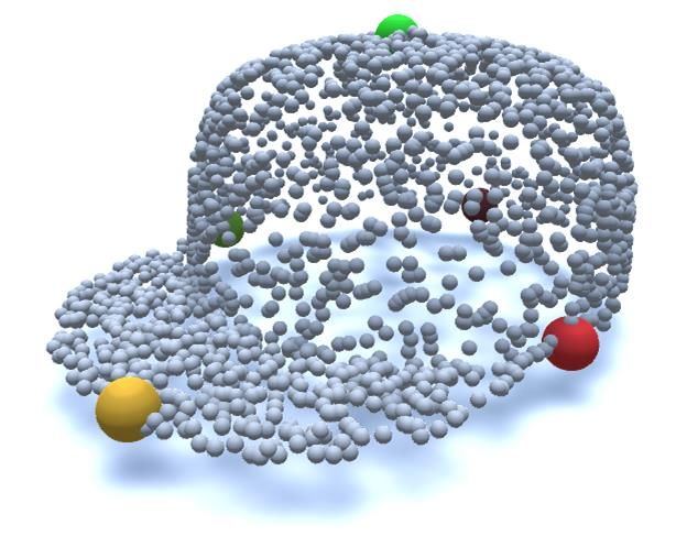
Dataset                Domain Correspondence Template-free Instances Categories Keypoints    Format
                                             √
         FAUST [4]              human                     ×             100       1        689K         mesh
                                             √
         SyncSpecCNN [42]        chair                    ×            6243       1       ∼60K      point cloud
                                                          √
         Dutagaci et al. [11]   general      ×                          43        16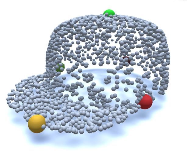
Airplane

            Bottle

             Cap

             Chair

          Skateboard

             Table

Figure 3. Dataset Visualization. Here we plot ground-truth keypoints for several categories. We can see that by utilizing our automatic
aggregation method, keypoints of high fidelity are extracted.

where dθ is the L2 distance between two vectors in embed-             robust to noisy points as the embedding space encodes the
ding space:                                                           semantic information of an object.
                                                                         Equation 1 involves both θ and Y and it is impractical
                dθ (a, b) = kgθ (a) − gθ (b)k22 ,
                                                                      to solve this problem in closed form. In practice, we use
and                                                                   alternating minimization with a deep neural network to ap-
                                                                      proximate the embedding function gθ , so that we solve the
                n∗ = arg min dθ (lm,n
                                  (c)
                                      , ym ).                         following dual problem instead (by slightly loosening the
                           n                                          constraints):
   Unlike previous methods such as Dutagaci et al.[11]
where a simple geodesic average of human labeled points
is given as ground-truth points, we seek a point whose ex-                θ∗ = arg min[H(gθ )
pected embedding distance to all human labeled points is                            θ
smallest. The reason is that geodesic distance is sensi-                                   Km
                                                                                         M X
                                                                                         X                                                (2)
tive to the misannotated keypoints and could not distinguish                    +λ                   kgθ (ym1 ,k ) − gθ (ym2 ,k )k22 ],
closely spaced keypoints, while embedding distance is more                              m1 ,m2   k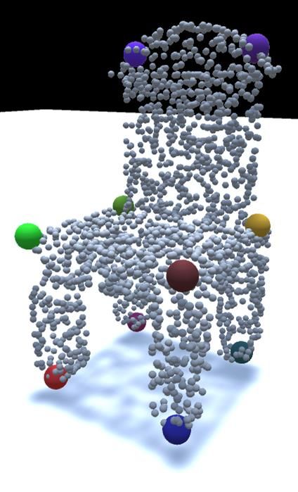
Fidelity Error
                                                                                            Calculatation

                    ……                                                  …...                                              ……
                Raw Annotations                                   Embedding Space                                   Fidelity Error Map

                                                                                                                              NMS

                                               Human                                         Clustering
                                             Verification                                      t-SNE

                    ……                                                                                                    ……
              Aggregated Keypoints                                Clustered Keypoints                              Potential Keypoints
Figure 4. Keypoint aggregation pipeline. We first infer dense embeddings from human labeled raw annotations. Then fidelity error maps
are calculated by summing embedding distances to human labeled keypoints. Non Minimum Suppression is conducted to form a potential
set of keypoints. These keypoints are then projected onto 2D subspace with t-SNE and verified by humans.

        Category       Train   Val   Test    All #Annotators                            Category          Train     Val    Test      All
        Airplane        715    102   205    1022     26                                 Airplane           9695    1379    2756    13830
        Bathtub         344     49    99    492      15                                 Bathtub            5519    772     1589     7880
        Bed             102     14    30    146       8                                 Bed                1276    188     377      1841
        Bottle          266     38    76    380       9                                 Bottle             4366    625     1269     6260
        Cap              26      4     8     38       6                                 Cap                154      24      48      226
        Car             701    100   201    1002     17                                 Car               14976    2133    4294    21403
        Chair           699    100   200    999      15                                 Chair              8488    1180    2395    12063
        Guitar          487     70   140    697      13                                 Guitar             4112    591     1197     5900
        Helmet           62     10    18     90       8                                 Helmet             529      85     162      776
        Knife           189     27    54    270       5                                 Knife              946     136     276      1358
        Laptop          307     44    88    439      12                                 Laptop             1842    264     528      2634
        Motorcycle      208     30    60    298       7                                 Motorcycle         2690    394     794      3878
        Mug             130     18    38    186       9                                 Mug                1427    198     418      2043
        Skateboard       98     14    29    141       9                                 Skateboard         903     137     283      1323
        Table           786    113   225    1124     17                                 Table              6325    913     1809     9047
        Vessel          637     91   182    910      18                                 Vessel             9168    1241    2579    12988
        Total          5757    824   1653   8234    194                                 Total             72416   10260   20774   103450

      Table 2. Keypoint Dataset statistics. Left: number of models in each category. Right: number of keypoints in each category.

                                                                               Non Minimum Suppression Equation 3 may be hard to
                                                                               solve since Km is also unknown beforehand. For each
                  M X
                  X   Km Z
                    C X                                     (c)
                                                        φ(lm,n? , x)           model Mm , the fidelity error associated with each poten-
Y ∗ = arg min                          dθ (x, ym,k )                 dx,       tial keypoint ym ∈ Mm is:
          Y      m=1 c=1 k=1     Mm                        Z(φ)
                                                                                               M X C Z                      (c)
                                                                                                                         φ(lm0 ,n∗ , x)
                 s.t. gθ (ym1 ,k ) ≡ gθ (ym2 ,k ), ∀m1 , m2 , k,
                                                                                               X
                                                                                f (ym , gθ ) =               dθ (x, ym )
                                                                                                                      0                 dx,
                                                                     (3)                       0  c=1 Mm0
                                                                                                                            Z(φ)
                                                                                              m 6=m
                                                                                                                                           (4)
and alternate between the two equations until convergence.
                                                                               where ym0 = arg minym0 ∈Mm0 kgθ (ym0 ) − gθ (ym )k22 .
   By solving this problem, we find both an optimal em-                           Then ym∗
                                                                                           is found by conducting Non Minimum Sup-
bedding function gθ , together with intra-class consistent                     pression (NMS), such that:
ground-truth keypoints Y, while keeping its embedding dis-
tance from human-labeled keypoints as close as possible.                                                      ∗
                                                                                                          f (ym , gθ ) ≤ f (ym , gθ ),
The ground-truth keypoints can be viewed as the projection                                                         ∗                       (5)
of human labeled data onto embedding space.                                                   ∀ym ∈ Mm , dθ (ym , ym ) < δ,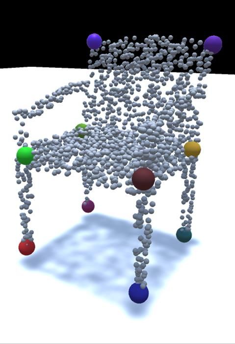
GroudTruth                     RSNet                        RSCNN                   DGCNN                    GraphCNN                      ISS3D                 HARRIS3D

             Table

             Chair

             Mug

                                                     Figure 5. Visualizations of detected keypoints for six algorithms.

             Airplane    Bathtub       Bed        Bottle       Cap         Car        Chair       Guitar      Helmet      Knife       Laptop      Motor        Mug         Skate      Table       Vessel     Average
PointNet     10.4/9.3     0.8/6.3     3.0/9.4     0.5/8.2     0.0/0.3     7.3/9.2     7.7/6.5     0.1/1.4     0.0/1.3     0.0/0.9    23.6/32.0    0.1/4.0     0.2/3.9      0.0/2.9   20.9/23.1    7.1/9.1     5.1/8.0
PointNet++   33.5/44.6   18.5/32.3   16.4/23.4   22.1/38.2   13.2/12.1   24.0/41.0   18.2/29.4   24.3/27.7    7.0/7.4    19.0/22.1   30.9/60.0   21.9/36.0   16.3/21.4   13.7/16.1   29.3/47.4   16.7/26.9   20.3/30.4
RSNet        33.7/38.8   23.1/36.0   28.4/42.5   29.4/44.3   26.7/26.9   30.4/42.3   22.7/26.2   30.5/34.2   15.8/21.3   21.7/31.5   39.8/62.0   31.5/43.2   24.1/35.2   21.6/25.9   39.7/54.6   18.3/22.3   27.3/36.7
SpiderCNN    24.6/24.7   13.0/16.4   16.4/17.1    3.6/8.2     0.0/0.5    11.8/17.2   18.2/20.4    7.4/9.9     0.0/0.5    14.9/18.7   25.6/40.0   12.0/13.3    2.2/4.0      1.8/3.3   27.9/40.5   12.9/14.6   12.0/15.6
PointConv    40.0/51.2   29.0/44.7   25.1/43.7   33.6/46.5    0.0/7.0    35.9/55.6   25.5/39.8   28.0/39.3    7.7/8.3    26.6/38.1   43.1/63.5   35.9/50.6   19.8/32.0    9.3/10.1   44.1/64.0   21.7/31.8   26.6/39.1
RSCNN        31.1/45.0   20.4/34.9   26.2/40.1   25.6/40.1    7.0/8.9    25.4/44.7   22.0/33.0   27.3/34.1    8.9/10.8   21.1/27.2   35.2/58.8   23.6/37.0   15.9/18.6   21.9/30.1   27.4/49.8   18.1/28.9   22.3/33.9
DGCNN        39.2/52.0   25.5/40.6   32.4/42.8   40.3/61.6    0.0/2.0    27.0/48.6   24.9/34.6   31.9/44.1   17.1/19.9   31.5/39.9   44.8/69.6   30.3/41.4   23.9/33.2   22.6/29.8   41.0/59.0   24.4/35.6   28.5/40.9
GraphCNN      0.7/0.7    17.0/23.7   22.2/31.5   23.3/42.6    0.0/4.1    23.0/36.5    0.6/0.6    17.0/21.6    9.7/12.5   18.7/23.3   33.3/49.7    0.6/0.7     0.5/0.6    11.7/12.8   24.5/34.7   15.1/19.3   13.6/19.7
Harris3D       1.6/-       0.3/-       0.9/-       0.5/-       0.0/-       0.9/-       0.7/-       1.2/-        0.0/-      1.9/-       0.3/-       0.7/-       0.0/-        1.0/-      0.4/-       1.2/-       0.7/-
SIFT3D         1.2/-       1.0/-       0.5/-       1.1/-       0.4/-       1.0/-       0.7/-       0.7/-        0.4/-      0.6/-       0.2/-       0.8/-       0.5/-        0.7/-      0.3/-       1.0/-       0.7/-
ISS3D          1.1/-       1.4/-       0.9/-       1.8/-       0.6/-       1.7/-       0.7/-       0.7/-        0.8/-      0.4/-       0.1/-       0.8/-       0.9/-        0.8/-      0.3/-       1.1/-       0.9/-

                          Table 3. mIoU and mAP results (in percentage) for compared methods with distance threshold 0.01.

where δ is some neighborhood threshold.                                                                       4.5. Pipeline
   After NMS, we would get several ground-truth points
ym,1 , ym,2 , . . . , ym,k for each manifold Mm . However, the                                                   The whole pipeline is shown in Figure 4. We first in-
arbitrarily assigned index k within each model does not pro-                                                  fer dense embeddings from human labeled raw annotations.
vide a consistent semantic correspondence across different                                                    Then fidelity error maps are calculated by summing em-
models. Therefore we cluster these points according to their                                                  bedding distances to human labeled keypoints. Non Min-
embeddings by first projecting them onto 2D subspace with                                                     imum Suppression is conducted to form a potential set of
t-SNE [21].                                                                                                   keypoints. These keypoints are then projected onto 2D sub-
                                                                                                              space with t-SNE and verified by humans.
Ground-truth Verification Though the above method
automatically aggregate a set of potential set of keypoints                                                   5. Tasks and Benchmarks
with high precision, it omits some keypoints in some cases.
As the last step, experts manually verify these keypoints                                                        In this section, we propose two keypoint prediction
based on some simple priors such as the rotational symme-                                                     tasks: keypoint saliency estimation and keypoint correspon-
try and centrosymmetry of an object.                                                                          dence estimation. Keypoint saliency estimation requires
                                                                                                              evaluated methods to give a set of potential indistinguish-
4.4. Implementation Details                                                                                   able keypoints while keypoint correspondence estimation
   At the start of the alternating minimization, we initialize                                                asks to localize a fixed number of distinguishable keypoints.
Y to be sampled from raw annotations and then run one it-
eration, which is enough for the convergence. We choose                                                       5.1. Keypoint Saliency Estimation
PointConv with hidden dimension 128 as the embedding
function g. During the optimization of Equation 3, we clas-                                                   Dataset Preparation For keypoint saliency estimation,
sify each point into K classes with a SoftMax layer and ex-                                                   we only consider whether a point is the keypoint or not,
tract the feature of the last but one layer as the embedding.                                                 without giving its semantic label. Our dataset is split into
The learning rate is 1e-3 and the optimizer is Adam [17].                                                     train, validation and test sets with the ratio 70%, 10%, 20%.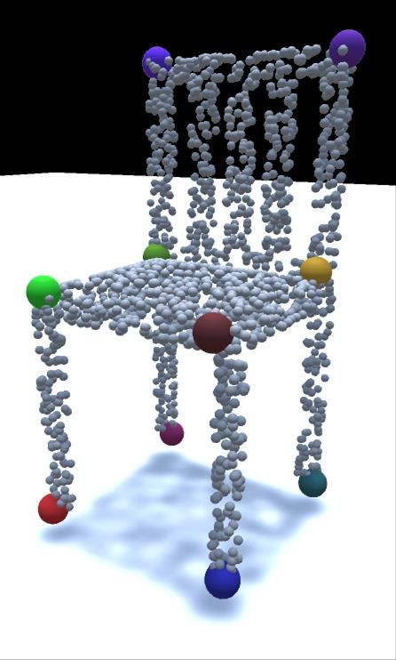
Evaluation Metrics Two metrics are adopted to evaluate
the performance of keypoint saliency estimation. Firstly, we
evaluate their mean Intersection over Unions [34] (mIoU),
which can be calculated as
                             TP
                IoU =                .                   (6)
                        TP + FP + FN
mIoU is calculated under different error tolerances from 0 to
0.1. Secondly, for those methods that output keypoint prob-
abilities, we evaluate their mean Average Precisions (mAP)
over all categories.

Benchmark Algorithms We benchmark eight state-
of-the-art algorithms on point cloud semantic analysis:
PointNet [27], PointNet++ [28], RSNet [13], Spider-
CNN [41], PointConv [39], RSCNN [20], DGCNN [38] and
                                                                Figure 6. mIoU results under various distance thresholds (0-0.1)
GraphCNN [10]. Three traditional local geometric keypoint
                                                                for compared algorithms.
detectors are also considered: Harris3D [31], SIFT3D [29]
and ISS3D [30].

Evaluation Results For deep learning methods, we use
the default network architectures and hyperparameters to
predict the keypoint probability of each point and mIoU and
mAP are adopted to evaluate their performance. For local
geometry based methods, mIoU is used. Each method is
tested with various geodesic error thresholds. In Table 3,
we report mIoU and mAP results under a restrictive thresh-
old 0.01. Figure 6 shows the mIoU curves under different
distance thresholds from 0 to 0.1 and Figure 7 shows the
mAP results. We can see that under a restrictive distance
threshold 0.01, geometric and deep learning methods both
fail to predict qualified keypoints.
    Figure 5 shows some visualizations of the results from
RSNet, RSCNN, DGCNN, GraphCNN, ISS3D and Har-
                                                                Figure 7. mAP results under various distance thresholds (0-0.1) for
ris3D. Deep learning methods can predict some of ground-
                                                                compared algorithms.
truth keypoints while the predicted keypoints are sometimes
missing. For local geometry based methods like ISS3D and
Harris3D, they give much more interest points spread over       number of keypoints is fixed and the data split is the same
the entire model while these points are agnostic of seman-      as keypoint saliency estimation.
tic information. Learning discriminative features for better
localizing accurate and distinct keypoints across various ob-
                                                                Evaluation Metric The prediction of network is evalu-
jects is still a challenging task.
                                                                ated by the percentage of correct keypoints (PCK), which
5.2. Keypoint Correspondence Estimation                         is used to evaluate the accuracy of keypoint prediction in
                                                                many previous works [42, 33].
   Keypoint correspondence estimation is a more challeng-
ing task, where one needs to predict not only the keypoints,
but also their semantic labels. The semantic labels should      Benchmark Algorithms We benchmark eight state-
be consistent across different objects in the same category.    of-the-art algorithms: PointNet [27], PointNet++[28],
                                                                RSNet [13], SpiderCNN [41], PointConv [39],
Dataset Preparation For keypoint correspondence esti-           RSCNN [20], DGCNN [38] and GraphCNN [10].
mation, each keypoint is labeled with a semantic index. For
those keypoints that do not exist on some objects, index -      Evaluation Results Similarly, we use the default network
1 is given. Similar to SyncSpecCNN [42], the maximum            architectures. Table 4 shows the PCK results with error dis-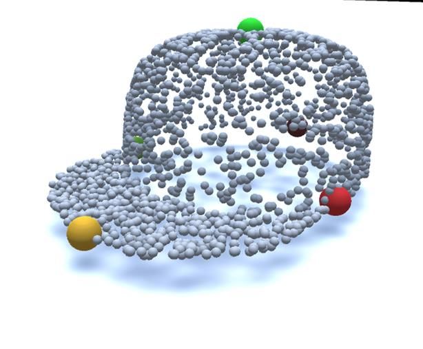
GroundTruth         PointNet               RSCNN       PointConv     SpiderCNN        DGCNN           GraphCNN

         Bathtub

         Helmet

       Motorbike

           Figure 8. Visualizations of detected keypoints and their semantic labels. Same colors indicate same semantic labels.

              Airplane   Bath   Bed    Bottle   Cap    Car    Chair Guitar Helmet Knife Laptop Motor   Mug    Skate   Table   Vessel Average
 PointNet       65.4     57.2   55.4    78.9    16.7   66.6    43.2 65.4    42.6 32.6 76.1      62.1   60.7    50.4    63.8    42.5   55.0
 PointNet++     64.1     45.4   44.2    10.2    18.8   55.1    38.0 55.4    23.6 43.8 64.6      49.9   36.4    42.3    57.1    37.9   42.9
 RSNet          68.9     56.0   69.2    78.2    47.9   65.7    49.4 63.7    33.8 56.9 80.3      67.4   61.7    69.2    72.3    46.7   61.7
 SpiderCNN      54.9     36.8   43.9    50.4     0.0   47.1    36.9 37.7    5.6   32.2 63.4     36.6   16.4    15.8    61.0    36.8   36.0
 PointConv      70.3     54.4   58.6    64.6    25.0   65.7    51.1 62.6    16.2 47.4 74.2      61.7   51.2    51.8    69.5    46.7   54.4
 RSCNN          66.8     47.9   52.4    59.4    18.8   56.5    45.0 60.0    21.3 51.4 66.9      52.8   29.5    51.7    64.8    41.2   49.2
 DGCNN          66.8     51.5   56.3     8.9    39.6   58.6    46.0 62.4    36.1 52.1 73.9      57.7   51.4    52.3    70.5    46.8   51.9
 GraphCNN       41.8     19.5   35.4    32.1     8.3   36.9    27.0 28.9    8.8   20.0 65.9     34.4   15.6    26.2    17.3    22.1   27.5

                          Table 4. PCK results under distance threshold 0.01 for various deep learning networks.

                                                                            ferent methods. Same colors denote same semantic labels.
                                                                            We can see that most methods can accurately predict some
                                                                            of keypoints. However, there are still some missing key-
                                                                            points and inaccurate localizations.
                                                                                Keypoint saliency estimation and keypoint correspon-
                                                                            dence estimation are both important for object understand-
                                                                            ing. Keypoint saliency estimation gives a spare represen-
                                                                            tation of object by extracting meaningful points. Key-
                                                                            point correspondence estimation establishes relations be-
                                                                            tween points on different objects. From the results above,
                                                                            we can see that these two tasks still remain challenging. The
                                                                            reason is that object keypoints from human perspective are
                                                                            not simply geometrically salient points but abstracts seman-
                                                                            tic meanings of the object.

Figure 9. PCK results under various distance thresholds (0-0.1) for         6. Conclusion
compared algorithms.
                                                                               In this paper, we propose a large-scale and high-quality
                                                                            KeypointNet dataset. In order to generate ground-truth key-
                                                                            points from raw human annotations where identification of
tance threshold 0.01. Figure 9 illustrates the percentage of                their modes are non-trivial, we transform the problem into
correct points curves with distance thresholds varied from                  an optimization problem and solve it in an alternating fash-
0 to 0.1. RS-Net performs relatively better than the other                  ion. By optimizing a fidelity loss, ground-truth keypoints,
methods under all thresholds. However, all eight methods                    together with their correspondences are generated. In addi-
face difficulty in giving exact consistent semantic keypoints               tion, we evaluate and compare several state-of-the-art meth-
under a threshold of 0.01.                                                  ods on our proposed dataset and we hope this dataset could
   Figure 8 shows some visualizations of the results for dif-               boost the semantic understanding of 3D objects.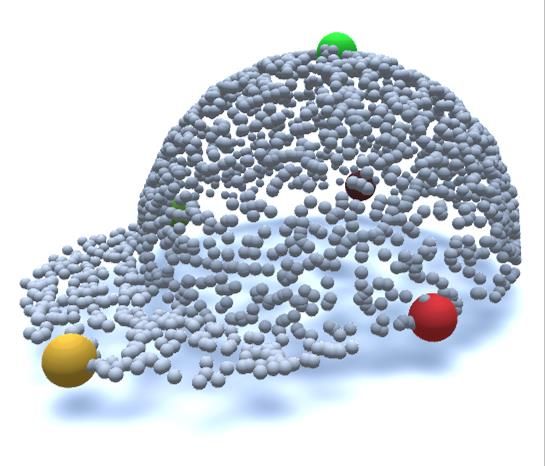
Acknowledgements                                                       [12] Hao-Shu Fang, Chenxi Wang, Minghao Gou, and Cewu
                                                                            Lu. Graspnet: A large-scale clustered and densely annotated
   This work is supported in part by the National Key                       datase for object grasping. arXiv preprint arXiv:1912.13470,
R&D Program of China (No. 2017YFA0700800), Na-                              2019. 2
tional Natural Science Foundation of China under Grants                [13] Qiangui Huang, Weiyue Wang, and Ulrich Neumann. Re-
61772332, 51675342, 51975350, SHEITC (2018-RGZN-                            current slice networks for 3d segmentation of point clouds.
02046) and Shanghai Science and Technology Commit-                          In Proceedings of the IEEE Conference on Computer Vision
tee.                                                                        and Pattern Recognition, pages 2626–2635, 2018. 7
                                                                       [14] Marc Khoury, Qian-Yi Zhou, and Vladlen Koltun. Learning
References                                                                  compact geometric features. In Proceedings of the IEEE In-
                                                                            ternational Conference on Computer Vision, pages 153–161,
 [1] Mscoco keypoint challenge 2016, 2016. 2
                                                                            2017. 2
 [2] Mykhaylo Andriluka, Umar Iqbal, Eldar Insafutdinov,
                                                                       [15] Vladimir G Kim, Wilmot Li, Niloy J Mitra, Siddhartha
     Leonid Pishchulin, Anton Milan, Juergen Gall, and Bernt
                                                                            Chaudhuri, Stephen DiVerdi, and Thomas Funkhouser.
     Schiele. Posetrack: A benchmark for human pose estima-
                                                                            Learning part-based templates from large collections of 3d
     tion and tracking. In Proceedings of the IEEE Conference
                                                                            shapes. ACM Transactions on Graphics (TOG), 32(4):70,
     on Computer Vision and Pattern Recognition, pages 5167–
                                                                            2013. 1, 2
     5176, 2018. 2
                                                                       [16] Vladimir G Kim, Wilmot Li, Niloy J Mitra, Stephen DiVerdi,
 [3] Mykhaylo Andriluka, Leonid Pishchulin, Peter Gehler, and
                                                                            and Thomas Funkhouser. Exploring collections of 3d models
     Bernt Schiele. 2d human pose estimation: New benchmark
                                                                            using fuzzy correspondences. ACM Transactions on Graph-
     and state of the art analysis. In IEEE Conference on Com-
                                                                            ics (TOG), 31(4):1–11, 2012. 3
     puter Vision and Pattern Recognition (CVPR), June 2014. 1,
                                                                       [17] Diederik P Kingma and Jimmy Ba. Adam: A method for
     2
                                                                            stochastic optimization. arXiv preprint arXiv:1412.6980,
 [4] Federica Bogo, Javier Romero, Matthew Loper, and                       2014. 6
     Michael J. Black. FAUST: Dataset and evaluation for 3D
                                                                       [18] Chang Ha Lee, Amitabh Varshney, and David W Jacobs.
     mesh registration. In Proceedings IEEE Conf. on Com-
                                                                            Mesh saliency. ACM transactions on graphics (TOG),
     puter Vision and Pattern Recognition (CVPR), Piscataway,
                                                                            24(3):659–666, 2005. 2
     NJ, USA, June 2014. IEEE. 3
                                                                       [19] Yong-Lu Li, Liang Xu, Xijie Huang, Xinpeng Liu, Ze Ma,
 [5] Lubomir Bourdev and Jitendra Malik. Poselets: Body part                Mingyang Chen, Shiyi Wang, Hao-Shu Fang, and Cewu Lu.
     detectors trained using 3d human pose annotations. In 2009             Hake: Human activity knowledge engine. arXiv preprint
     IEEE 12th International Conference on Computer Vision,                 arXiv:1904.06539, 2019. 2
     pages 1365–1372. IEEE, 2009. 2                                    [20] Yongcheng Liu, Bin Fan, Shiming Xiang, and Chunhong
 [6] M Bueno, J Martı́nez-Sánchez, H González-Jorge, and H                Pan. Relation-shape convolutional neural network for point
     Lorenzo. Detection of geometric keypoints and its applica-             cloud analysis. In Proceedings of the IEEE Conference
     tion to point cloud coarse registration. International Archives        on Computer Vision and Pattern Recognition, pages 8895–
     of the Photogrammetry, Remote Sensing & Spatial Informa-               8904, 2019. 7
     tion Sciences, 41, 2016. 1                                        [21] Laurens van der Maaten and Geoffrey Hinton. Visualiz-
 [7] Umberto Castellani, Marco Cristani, Simone Fantoni, and                ing data using t-sne. Journal of machine learning research,
     Vittorio Murino. Sparse points matching by combining                   9(Nov):2579–2605, 2008. 6
     3d mesh saliency with statistical descriptors. In Computer        [22] Ajmal S Mian, Mohammed Bennamoun, and Robyn Owens.
     Graphics Forum, volume 27, pages 643–652. Wiley Online                 Three-dimensional model-based object recognition and seg-
     Library, 2008. 2                                                       mentation in cluttered scenes. IEEE transactions on pattern
 [8] Angel X Chang, Thomas Funkhouser, Leonidas Guibas,                     analysis and machine intelligence, 28(10):1584–1601, 2006.
     Pat Hanrahan, Qixing Huang, Zimo Li, Silvio Savarese,                  1
     Manolis Savva, Shuran Song, Hao Su, et al. Shapenet:              [23] Juhong Min, Jongmin Lee, Jean Ponce, and Minsu Cho.
     An information-rich 3d model repository. arXiv preprint                Spair-71k: A large-scale benchmark for semantic correspon-
     arXiv:1512.03012, 2015. 2                                              dence. arXiv preprint arXiv:1908.10543, 2019. 1, 2
 [9] Taco S Cohen, Mario Geiger, Jonas Köhler, and Max                [24] John Novatnack and Ko Nishino. Scale-dependent 3d geo-
     Welling. Spherical cnns. arXiv preprint arXiv:1801.10130,              metric features. In 2007 IEEE 11th International Conference
     2018. 2                                                                on Computer Vision, pages 1–8. IEEE, 2007. 2
[10] Michaël Defferrard, Xavier Bresson, and Pierre Van-              [25] Bo Pang, Kaiwen Zha, Yifan Zhang, and Cewu Lu. Further
     dergheynst. Convolutional neural networks on graphs with               understanding videos through adverbs: A new video task. In
     fast localized spectral filtering. In Advances in neural infor-        AAAI, 2020. 2
     mation processing systems, pages 3844–3852, 2016. 7               [26] Georgios Pavlakos, Xiaowei Zhou, Aaron Chan, Konstanti-
[11] Helin Dutagaci, Chun Pan Cheung, and Afzal Godil. Eval-                nos G Derpanis, and Kostas Daniilidis. 6-dof object pose
     uation of 3d interest point detection techniques via human-            from semantic keypoints. In 2017 IEEE International Con-
     generated ground truth. The Visual Computer, 28(9):901–                ference on Robotics and Automation (ICRA), pages 2011–
     917, 2012. 1, 2, 3, 4                                                  2018. IEEE, 2017. 2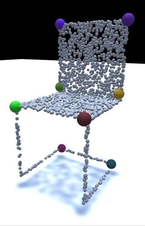
[27] Charles R Qi, Hao Su, Kaichun Mo, and Leonidas J Guibas.         [41] Yifan Xu, Tianqi Fan, Mingye Xu, Long Zeng, and Yu Qiao.
     Pointnet: Deep learning on point sets for 3d classification           Spidercnn: Deep learning on point sets with parameterized
     and segmentation. In Proceedings of the IEEE Conference on            convolutional filters. In Proceedings of the European Con-
     Computer Vision and Pattern Recognition, pages 652–660,               ference on Computer Vision (ECCV), pages 87–102, 2018.
     2017. 7                                                               7
[28] Charles Ruizhongtai Qi, Li Yi, Hao Su, and Leonidas J            [42] Li Yi, Hao Su, Xingwen Guo, and Leonidas J Guibas. Sync-
     Guibas. Pointnet++: Deep hierarchical feature learning on             speccnn: Synchronized spectral cnn for 3d shape segmenta-
     point sets in a metric space. In Advances in neural informa-          tion. In Proceedings of the IEEE Conference on Computer
     tion processing systems, pages 5099–5108, 2017. 7                     Vision and Pattern Recognition, pages 2282–2290, 2017. 1,
[29] Blaine Rister, Mark A Horowitz, and Daniel L Rubin.                   2, 3, 7
     Volumetric image registration from invariant keypoints.          [43] Yang You, Yujing Lou, Qi Liu, Yu-Wing Tai, Weiming
     IEEE Transactions on Image Processing, 26(10):4900–4910,              Wang, Lizhuang Ma, and Cewu Lu. Prin: Pointwise rotation-
     2017. 7                                                               invariant network. arXiv preprint arXiv:1811.09361, 2018.
[30] Samuele Salti, Federico Tombari, Riccardo Spezialetti, and            2
     Luigi Di Stefano. Learning a descriptor-specific 3d keypoint
     detector. In Proceedings of the IEEE International Confer-
     ence on Computer Vision, pages 2318–2326, 2015. 7
[31] Ivan Sipiran and Benjamin Bustos. Harris 3d: a robust ex-
     tension of the harris operator for interest point detection on
     3d meshes. The Visual Computer, 27(11):963, 2011. 2, 7
[32] Jian Sun, Maks Ovsjanikov, and Leonidas Guibas. A concise
     and provably informative multi-scale signature based on heat
     diffusion. In Computer graphics forum, volume 28, pages
     1383–1392. Wiley Online Library, 2009. 2
[33] Minhyuk Sung, Hao Su, Ronald Yu, and Leonidas J Guibas.
     Deep functional dictionaries: Learning consistent semantic
     structures on 3d models from functions. In Advances in Neu-
     ral Information Processing Systems, pages 485–495, 2018.
     2, 7
[34] Leizer Teran and Philippos Mordohai. 3d interest point de-
     tection via discriminative learning. In European Conference
     on Computer Vision, pages 159–173. Springer, 2014. 7
[35] Federico Tombari, Samuele Salti, and Luigi Di Stefano.
     Unique signatures of histograms for local surface descrip-
     tion. In European conference on computer vision, pages
     356–369. Springer, 2010. 2
[36] C. Wah, S. Branson, P. Welinder, P. Perona, and S. Belongie.
     The Caltech-UCSD Birds-200-2011 Dataset. Technical Re-
     port CNS-TR-2011-001, California Institute of Technology,
     2011. 2
[37] Hanyu Wang, Jianwei Guo, Dong-Ming Yan, Weize Quan,
     and Xiaopeng Zhang. Learning 3d keypoint descriptors for
     non-rigid shape matching. In Proceedings of the European
     Conference on Computer Vision (ECCV), pages 3–19, 2018.
     1
[38] Yue Wang, Yongbin Sun, Ziwei Liu, Sanjay E Sarma,
     Michael M Bronstein, and Justin M Solomon. Dynamic
     graph cnn for learning on point clouds. ACM Transactions
     on Graphics (TOG), 38(5):146, 2019. 7
[39] Wenxuan Wu, Zhongang Qi, and Li Fuxin. Pointconv: Deep
     convolutional networks on 3d point clouds. In Proceedings
     of the IEEE Conference on Computer Vision and Pattern
     Recognition, pages 9621–9630, 2019. 7
[40] Yu Xiang, Roozbeh Mottaghi, and Silvio Savarese. Beyond
     pascal: A benchmark for 3d object detection in the wild. In
     IEEE Winter Conference on Applications of Computer Vision
     (WACV), 2014. 3
You can also read