A PRIORI GUARANTEES OF FINITE-TIME CONVER-GENCE FOR DEEP NEURAL NETWORKS - OpenReview
←
→
Page content transcription
If your browser does not render page correctly, please read the page content below
Under review as a conference paper at ICLR 2021

A PRIORI GUARANTEES OF FINITE - TIME CONVER -
GENCE FOR D EEP N EURAL N ETWORKS

 Anonymous authors
 Paper under double-blind review

                                            A BSTRACT

         In this paper, we perform Lyapunov based analysis of the loss function to derive an
         a priori upper bound on the settling time of deep neural networks. While previous
         studies have attempted to understand deep learning using control theory frame-
         work, there is limited work on a priori finite time convergence analysis. Drawing
         from the advances in analysis of finite-time control of non-linear systems, we
         provide a priori guarantees of finite-time convergence in a deterministic control
         theoretic setting. We formulate the supervised learning framework as a control
         problem where weights of the network are control inputs and learning translates
         into a tracking problem. An analytical formula for finite-time upper bound on
         settling time is provided a priori under the assumptions of boundedness of input.
         Finally, we prove that our loss function is robust against input perturbations.

1   I NTRODUCTION
Over the past decade, Deep neural networks have achieved human-like performance in various ma-
chine learning tasks, such as classification, natural language processing and speech recognition.
Despite the popularity of deep learning, the underlying theoretical understanding remains relatively
less explored. While attempts have been made to develop deep learning theory by drawing inspi-
ration from other related fields such as statistical learning and information theory, a comprehensive
theoretical framework is still in an early developmental stage. It is difficult to perform mathematical
analysis on Deep neural networks due to the large number of parameters involved. Other problems
in deep neural networks revolve around the stability and desired convergence rate of the training.
Since the performance of the network depends highly on the training data and the choice of the opti-
mization algorithm, there is no guarantee that the training will converge. Our work attempts to give
finite-time convergence guarantees for training of a deep neural network by utilizing an established
stabilization framework from control theory.
Existing works in deep learning theory have attempted to bridge the gap in understanding deep
learning dynamics by focusing on simple models of neural networks [Saxe et al. (2013), Li & Yuan
(2017), Arora et al. (2018), Jacot et al. (2018)]. This could be attributed to the fact that current
state-of-the-art deep learning models are highly complex structures to analyze. Jacot et al. (2018)
proved that a multilayer fully-connected network with infinite width converges to a deterministic
limit at initialization and the rate of change of weights goes to zero. Saxe et al. (2013) analyzed
deep linear networks and proved that these networks, surprisingly, have a rich non-linear structure.
The study shows that given the right initial conditions, deep linear networks are a finite amount
slower than shallow networks. Following this work, Arora et al. (2018) proved the convergence of
gradient descent to global minima for networks with dimensions of every layer being full rank in di-
mensions. While these studies give important insights into the design of neural network architecture
and the behavior of training, their results may need to be modified in order to provide convergence
guarantees for the conventional deep neural networks. Du et al. (2018) extended the work of Jacot
et al. (2018) further by proving convergence for gradient descent to achieve zero training loss in
deep neural networks with residual connections.
When it comes to convergence of certain state variables of a dynamical system, control theory pro-
vides a rich mathematical framework which can be utilized for analyzing the non-linear dynamics
of deep learning [Liu & Theodorou (2019)]. One of the early works relating deep learning to con-
trol theory was of LeCun et al. (1988), which used the concept of optimal control and formulated

                                                  1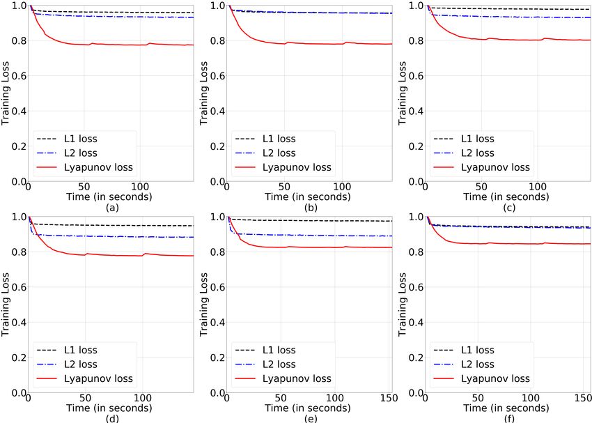
Under review as a conference paper at ICLR 2021

back-propagation as an optimization problem with non-linear constraints. Non-linear control has
gained increasing attention over the past few years in the context of neural networks, especially for
recurrent neural networks [Allen-Zhu et al. (2019), Xiao (2017)] and reinforcement learning [Xu
et al. (2013), Gupta et al. (2019), Wang et al. (2019), Kaledin et al. (2020)]. A new class of recurrent
neural networks, called Zhang Neural Networks (ZNN), was developed that expressed dynamics of
the network as a set of ordinary differential equations and used non-linear control to prove global
or exponential stability for time-varying Sylvester equation [Zhang et al. (2002), Guo et al. (2011)].
Li et al. (2013) introduced the sign bi-power activation function for Zhang Neural Networks (ZNN)
which helps to prove the existence of finite-time convergence property. Haber & Ruthotto (2017)
presents deep learning as a parameter estimation problem of non-linear dynamical systems to tackle
the exploding and vanishing gradients.
The focus of this paper is on deriving a priori guarantee of attaining finite-time convergence of train-
ing in a supervised learning framework under some assumptions on inputs. The novelty lies in the
fact that the weight update is cast as a finite-time control synthesis such that the loss function is
proven to be a valid Lyapunov function. The resulting training update is derived as a function of
time such that it ensures the convergence of Lyapunov function in finite time. The only assumption
used is that the magnitude of atleast one input is greater than zero. Thus, the learning problem is
converted into a finite time stabilization problem as studied rigorously in Bhat & Bernstein (2000).
The contributions of the proposed study are twofold. First, we propose a Lyapunov candidate func-
tion to be used as loss function. Second, we modify the weight update of the neural network in
such a way that the supervised training is converted into a dynamical control system. This allows
us to use results from Bhat & Bernstein (2000) to a priori guarantee finite time convergence on the
training. To the best of our knowledge, a guarantee of finite-time convergence is being studied for
the first time in context of training a general multi-layer neural network. The proposed results will
enable time bound training that will be useful in real-time applications.
The paper is organized as follows. Section 2 starts with introducing the Lyapunov function from
the control theory perspective. Section 2.1 derives the weight update and lyapunov loss function
for a single neuron case and proves that it satisfies the conditions required for finite-time stability
theorems developed in Bhat & Bernstein (2000) to be applicable. Section 2.2 then proves that
a similar result extends to a multi-layer perceptron network under reasonable assumptions on the
input. In Section 2.3, we state the equations to compute upper bounds on the convergence time for
training neural networks. Section 2.4 provides an extension to the case when bounded perturbations
are admitted at the input and convergence guarantees are shown to hold true. In Section 3, some
numerical simulations are presented for both single neuron and multi-layer perceptron cases for
regression. Section 4 collects conclusions and discusses future scope.

2     P ROPOSED METHOD TO CONVERT SUPERVISED LEARNING INTO
      DYNAMICAL CONTROL SYSTEM

This section motivates the development of a priori bounds on settling time with certain assumptions
on the input. The weight update problem for supervised learning in neural networks is similar to
the tracking problem of non-linear control systems. The idea is to synthesize a feedback control law
based on certain Lyapunov function V (x). A Lyapunov function is a positive definite function, i.e.
V (x) > 0, and its time derivative is negative definite along the given system dynamics, i.e. V̇ < 0.
We cast the supervised learning problem as a dynamical system which admits a valid Lyapunov
function as the loss function with the weight update is designed as a function of time.

2.1   S INGLE N EURON C ASE

We start with a simplistic single neuron case. Let x ∈ Rn be the input to the network where
                         >
x = [x1 x2 · · · xn ] , |xi | < c, i = 1, 2, · · · n holds
                                                      Pn true for some a priori but arbitrary scalar
c ∈ (0, ∞). Let y ? be the target output and z =         i=1 wi xi + b be the linear combination of
weights wi with inputs xi and bias b. The definition of signum function used here is sign(x) =
1, ∀x > 0, sign(x) = −1, ∀x < 0, sign(x) ∈ [−1, 1], x = 0. For our analysis, we choose sigmoid
function as our activation function, i.e. σ(z) = 1+e1−z . The output of the neural network is given
by y = σ(z). Let the error in output be defined as ē = y − y ∗ . The first objective is to convert our

                                                   2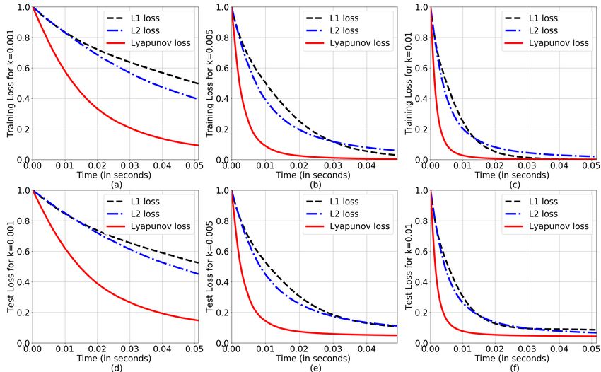
Under review as a conference paper at ICLR 2021

loss function into a candidate Lyapunov function in order to apply the control theoretic principles.
Consider a continuous function E(ē) to be a candidate Lyapunov function as follows:
                                                       |ē|(α+1)
                                               E=                                                          (1)
                                                       (α + 1)
where α ∈ (0, 1) is a user-defined parameter. The second objective is to define the temporal rate of
weight as the control input to enforce the stability of the origin ē = 0 as t → ∞. The Lyapunov
function in (1) is used to show that it is indeed plausible to achieve this asymptotic stability goal.
Taking the temporal derivative of the candidate Lyapunov function (1) produces (by chain rule of
differentiation)
                                      dE      dE dē dy dz dw
                                            =
                                       dt     dē dy dz dw dt
            dē dy dz
where dEdē dy dz dw is the weight update for standard gradient descent algorithm and
                                                                                              dw
                                                                                              dt   is the addi-
tional term we introduce to the weight update equation. Using (1), we get:
                                             e−z

                    dE
                       = |ē|α sign(ē)                 (x1 ẇ1 + x2 ẇ2 + · · · + xn ẇn )                (2)
                    dt                    (1 + e−z )2
Define, u1 , ẇ1 , u2 , ẇ2 , · · · , un , ẇn , and
                      ui = −ki sign(xi ) sign(ē)ez (1 + e−z )2 ,    i = 1, 2, · · · , n,                  (3)
where ki > 0, for all i, are tuning parameters to be chosen by the user. It can be noted that all control
inputs u1 , u2 , · · · , un remain bounded due to boundedness assumption of all the inputs xi and that
of ez . Substituting (3) into (2) produces
                                                       n
                                                                  !
                                        dE         α
                                                      X
                                            = −|ē|       ki |xi |                                    (4)
                                        dt            i=1

Assumption 1. At least one input of all xi , i = 1, 2, · · · , n is non-zero such that |xj | > γ > 0
where γ is a priori known scalar for some integers j ∈ [1, n].

It can be noted that Assumption 1 is reasonable for many practical applications in that some inputs
will always be nonzero with a known lower bound on its magnitude. First main result of the paper
is in order.
Theorem 1. Assuming Assumption 1 holds true, let the output of the neural network be given by
y = σ(z). Let all the inputs xi , i = 1, 2, · · · , n be bounded by some a priori known scalar a ∈
(0, ∞) such that |xi | < a holds true for all i. Then, weight update (3) causes the error ē = y − y ∗
to converge to zero in finite time.

Proof. The proof of the theorem is furnished using standard Lyapunov analysis arguments. Consider
E defined by (1) as a candidate Lyapunov function. Observing (4), it can be concluded that the right
hand side of the temporal derivative of remains negative definite since it involves power terms and
norm of inputs. Furthermore, (4) can be rewritten under the assumption 1 as follows:
                                             dE
                                                ≤ −kmin γE β                                               (5)
                                             dt
                                                 α
                                                                        α
where kmin = min(ki ), i = 1, 2, · · · , n, β = α+1 and |ē|α = |ē|α+1 α+1 = E β has been utilized.
Noting that E is a positive definite function and scalars kmin and γ are always positive, the proof is
complete by applying (Bhat & Bernstein, 2000, Theorem 4.2).

2.2   M ULTI N EURON C ASE

Consider a multi-layer perceptron with N layers where the layers are connected in a feed-forward
manner (Bishop, 1995, Chapter 4). Let x ∈ Rn be the input to the network where x =
                   >
[x1 x2 · · · xn ] and |xi | < c, i = 1, 2, · · · n holds true for some a priori but arbitrary scalar c ∈
                  m
(0, ∞). Let y ∈ R define the multi-neuron output to the network where y = [y1 y2 · · · ym ].
Let y ? ∈ Rm define the target output values of the network where y ? = [y1? y2? · · · ym       ?
                                                                                                  ]. The

                                                       3
Under review as a conference paper at ICLR 2021
error in the output layer can be expressed as ē = [|y1 − y1? | |y2 − y2? | ··· ?
|ym − ym |]. Hence,
the scalar candidate Lyapunov function can be written as follows:
|ē1 |(α+1) |ēm |(α+1)
E = E1 + · · · + Em = + ··· + (6)
(α + 1) (α + 1)
As is usually done in the case of feed-forward networks, consider unit j of layer l that computes its
output
X
alj = l l
wji zi (7)
i
using its inputs zil from layer l where bias parameter has been embedded inside the linear combi-
nation and zjl = σ(al−1 j ), where σ is non-linear activation function. The aim of this section is to
extend the single neuron case to a multi-neuron one. The simplest way do achieve this is to find
l
sensitivity of E to the weight wji of a given layer l, which is given by
∂Em ∂Em ∂alj
l
= (8)
∂wji ∂alj ∂wji
l
∂Em
Using standard notation δjl , ∂alj
with (7) results in:
∂Em
l
= δjl zil (9)
∂wji
L
It is straightforward to compute δm that belongs to the output layer L as shown below:
∂Em ∂Em
L
δm = L
= σ 0 (aL
m) (10)
∂am ∂ym
L
where zm is replaced by ym as it is the output layer. Finally, computation of δjl for all hidden units
is given by
∂Em X ∂Em ∂al+1
δjl = l
= k
(11)
∂aj k
∂al+1
k
∂alj
where units with a label k includes either hidden layer units or an output unit in layer l + 1. Com-
bining (7), zjl = σ(alj ) and δjl , ∂E
∂al
m
produces
j
X
δjl = σ 0 (alj ) l+1 l+1
wkj δk (12)
k
A slightly modified version of assumption 1 is required before the next result of the paper is pre-
sented.
Assumption 2. At least one input of all zi , i = 1, 2, · · · , L is non-zero such that |zn | > γ > 0
where γ is a priori known scalar for some integers n ∈ [1, L] where L is the number of units in layer
l.
Theorem 2. Let the weight update for connecting unit i of layer l to unit j of layer l + 1 of a
multi-layer neural network be given by
l l
ẇji = −kji sign(δjl zil )|δjl zil |α E β (13)
with some scalar β ∈ (0, 1) such that α + β < 1 and kji > 0 is a tuning parameter. Then the output
vector y converges to y ∗ in finite time.
Proof. Consider the candidate Lyapunov function E given by (6). The temporal derivative of the
Lyapunov function is given by
X X ∂Em
l
Ė = Ėm = ẇji (14)
m m
∂w jil
4Under review as a conference paper at ICLR 2021
which can be simplified using (13) and (9) as
X
Ė = −E β l
kji |δjl zil |α+1 (15)
m
l
Using Assumption 2 it is easy to conclude that for some kmin = min kji > 0, the following inequal-
i,j,l
ity holds true:
Ė ≤ −kmin γ α+1 E β (16)
Noting that E is a positive definite function and scalars kmin , γ are always positive, the proof is
complete by applying (Bhat & Bernstein, 2000, Theorem 4.2).
Remark 1. It can be seen that weight update (13) (or respectively (3)) is in a feedback control form
where state zi and δj (respectively xi and ē) are being used for influencing the learning process.
2.3 S ETTLING TIME FOR NEURAL NETWORK TRAINING
Theorem 1 and 2 prove that using candidate Lyapunov function as the loss function and the temporal
rate of change of the loss function as the weight update equation, we can convert supervised learning
framework into a control problem. (Bhat & Bernstein, 2000, Theorem 4.2) states that if there is
continuous function that is positive definite and it’s rate of change with respect to time is negative
definite, then it’s finite time stable equilibrium is at origin. The theorem also gives the settling time
when the above conditions are satisfied by the control system. For our case, this means that the
Lyapunov based loss function will converge in finite time and time taken to converge is as given
below:
The settling time for Single Neuron case:
1 (1−β)
T ≤ E (17)
kmin γ(1 − β) ini
The settling time for Multi Neuron case:
1 (1−β)
T ≤ E (18)
kmin γ α+1 (1 − β) ini
where γ is the lower bound on the inputs, kmin is the minimum value of tuning parameter k, α is
the scalar used in the Lyapunov loss function and Eini is the initial value of loss, i.e. loss at t = 0.
2.4 S ENSITIVITY TO PERTURBATIONS
This section considers the robustness of training a neural network based on our proposed algorithm.
In control theoretic terms, perturbation can be understood either as a disturbance to the process or as
modelling uncertainty. When supervised learning is viewed as a control process, perturbation in each
neuron of the input layer can be seen as external noise. This perturbation could cause the control
system to diverge. In this section, we develop theoretical claims that even with perturbed inputs,
training a neural network with the proposed algorithm will converge. The following assumption of
the upper bound on the perturbation of inputs is invoked.
Assumption 3. There exists an a priori known constant M > 0 such that all inputs xi , i =
1, 2, · · · , N admit additive perturbations ∆xi such that
|∆xi | ≤ M |xi |α (19)
for all i where N is the number of inputs.
The following result is in order.
Theorem 3. Let assumptions 2 and 3 hold true. Let the weight update for connecting unit i of layer
l to unit j of layer l + 1 of a multi-layer neural network be given by (13). Then the output vector y
converges to y ∗ in finite time in the presence of additive perturbations ∆xn , n ∈ [1, L] if kmin > M .
5Under review as a conference paper at ICLR 2021
Proof. It can be seen that the perturbation is considered only in inputs. Hence all hidden layer
weights are updated as done in the proof of Theorem 2. Hence, the dynamics of learning results in
the following revised temporal derivative of Lyapunov function:
X n
X
β α+1
Ė = −E kji |δj zi | + k1p |δp xp |α sign(δp xp )δp ∆xp (20)
m p=0
where k1p is the gain parameter for training of all the input layer weights. The expression in (20)
can be simplified using Assumption 3 as follows:
X n
X
Ė ≤ −E β kji |δj zi |α+1 + E β k1p |δp xp |α+1 M,
m p=0 (21)
X
β α+1
≤ −E (kji − M )|δj zi |
m
where inputs zi now collect inputs xi as well. Similar to the proof of Theorem 2, (21) can be
re-written by applying Assumption 2 as follows:
Ė ≤ −(kmin − M )γE β (22)
Since kmin > M , the proof is complete by applying (Bhat & Bernstein, 2000, Theorem 4.2).
3 E XPERIMENTS
This section presents empirical evidence that the theoretical results derived in the above sections
hold for real-life applications.
Convergence Rate for training. To analyze the training convergence rate of the proposed method,
we train a multi-layer perceptron (covered in Section 2.2) to perform regression on the Boston
Housing dataset (Harrison Jr & Rubinfeld (1978)). Experiment on single neuron case is covered
in Appendix A.2.2
Training details. We compare our proposed method (Lyapunov based loss and modified weight
update equation) with traditional L1 , L2 loss functions and standard SGD weight update equa-
tion. The modifications to the weight update equation for Lyapunov loss are as stated in (15)
for multi-neuron case. We plot the training and test loss with respect to time in Figure 1.
The details about the training examples,
epochs, learning rate etc. are specified under
the description of the figures. We observe that
the Lyapunov Loss function converges faster
than L1 and L2 loss functions, demonstrating
the results proven extensively in Section 2. This
is attributed mainly to the non-Lipschitz weight
updates given by (3) and (13).
The settling time as well as metrics of the
trained networks are reported in Table 1. The
time taken by the proposed algorithm to con-
verge falls within the a priori upper bound. We
also observe that the metrics (Accuracy for sin-
gle neuron case and rmse (Root mean square er-
ror) for multi-neuron case) achieved by the pro-
posed method is better than the baselines. Ad-
mittedly, the theoretical upper bound on settling
time for single neuron and multi-layer percep-
tron produced by (5) and (16) are very conser- Figure 1: Comparison of convergence with re-
vative, yet it is an a priori deterministic upper spect to time for the multi-layer perceptron trained
bound and the aggressive learning proves to be on the Boston Housing dataset. All networks are
faster than traditional loss functions in the sce- trained for 4000 epochs with learning rate = 0.02
narios considered here. and α = 0.68.
6Under review as a conference paper at ICLR 2021
Experiment Theoretical Upper Exp. Convergence Time Metric
Bound (in seconds)
(in seconds) L1 L2 Lyap. L1 L2 Lyap.
SingleNeuron (acc) ∼ 3.4e3 0.065 0.064 0.025 0.95 0.95 1.0
MLP (rmse) ∼ 1.4e10 4.3e3 3.4e3 3.1e3 0.091 0.179 0.085
Table 1: Settling time in seconds for each experiment conducted. We compare the time taken for
convergence by three different loss functions, L1 , L2 and Lyapunov Loss function. The training
conditions were similar for individual cases in the experiment. The single neuron case is trained on
Iris dataset and the metric used is Accuracy (higher is better). For Multi-layer perceptron, we use
Boston Housing dataset and the metric used for this is rmse (lower is better).
This can be attributed to the fact that we operate in the realm of non-smooth functions which tend
to be more aggressive than the smooth L2 function we usually encounter in most learning problems.
We can clearly observe that the loss value does not converge to zero. According to (Bhat & Bern-
stein, 2000, Theorem 5.2), a control system will converge to a non-zero value at steady state, if there
is constant perturbation in the input. Usually in real life datasets, there is an inherent bias or constant
perturbation, which prevents the loss to converge to zero. Of course, by setting α = 0, we can reject
all persisting disturbances (Orlov (2005)) and force the loss to converge to zero, but this may result
in discontinuity in back propagation (discussed in Appendix A.1) and result into large numerical
errors.
Hyperparameter analysis and its effect on training. In this section, we attempt to give an em-
pirical analysis as to how changes in the hyperparameters like k and α affect the training of the
neural network. In order to study the effect of tuning k, we work with the single neuron case for
simplicity and ease of understanding. We use Iris dataset for this experiment Dua & Graff (2017).
Existing literature in control theory suggests that a monotonic increase in the tuning parameter, k
should result in a monotonic decrease in the corresponding loss. In neural network terminology, k
can be considered as the ’learning rate’. We can clearly see in Figure 2 that k behaves like learning
rate parameter where increasing k makes the learning more aggressive.
Figure 2: Comparison of training and test convergence with respect to time for different values of
tuning parameter, k in a single neuron trained on the Iris dataset. We convert the problem into a
binary classification problem by considering only two output classes. All networks are trained for
600 epochs with 80 training examples and 20 test examples. The learning rate for all L1 , L2 and
Lyapunov is set to the tuning parameter value k and α = 0.8
From Table 2, we observe that the settling time for the training loss of our Lyapunov loss function
is always less than L1 and L2 . We also observe that the Accuracy of our method is either better
7Under review as a conference paper at ICLR 2021
or similar to the baselines, which shows that the optimized solution achieved by our method is
l
either better or on par with the baselines. For the multi-neuron case, we have defined kij for every
l
weight. Similar to adaptive learning rate, we can either tune kij for every weight (which can be quite
cumbersome for larger neural networks) or we can set it arbitrarily to the same value for all weights.
l
It must be noted that kij can be set to any value greater than an a priori known positive constant M .
Experiment Theoretical Upper Exp. Convergence Time Accuracy
for single Bound (in seconds) on Test Set
neuron case (in seconds) L1 L2 Lyap. L1 L2 Lyap.
on Iris dataset
k = 0.001 ∼ 37213.848 0.312 0.310 0.0918 0.6 0.95 0.95
k = 0.005 ∼ 7442.769 0.0943 0.0942 0.0344 0.95 1.0 1.0
k = 0.01 ∼ 3721.385 0.0566 0.0573 0.0221 0.95 1.0 1.0
Table 2: Settling time in seconds for different values of tuning parameter, k for the single neuron
case on Iris dataset. We compare the time taken for convergence by three different loss functions,
L1 , L2 and Lyapunov Loss function. The training conditions were similar for individual cases in the
experiment.
We will discuss the impact of different values of α on the training process of our neural network.
For the given experiments, we tested the network for various values of α ranging between (0, 1). We
observed that the training loss follows equations proved in above sections as long as α ∈ (0.5, 0.9).
If α happens to be too close to zero, the resulting control law becomes discontinuous thereby
resulting in numerical instabilities owing to the fact that the current ODE solvers are unable to
handle functions that are discontinuous. More details about the case α = 0 is given in Appendix
A.1 (Bhat & Bernstein, 2000, Theorem 5.2).
Stability of learning in the presence of amplitude-bounded perturbations.
Figure 3: Comparison of training loss convergence with respect to time for different values of input
perturbations, ∆x for a multi-layer perceptron trained on the IMDB Wiki Faces dataset.The a priori
upper bound on input perturbations are as follows: (a) ∆x = 0.1, (b) ∆x = 0.2, (c)∆x = 0.3
Learning rate/k = 0.0009, α = 0.8, epochs=100
In this section, we present results that demonstrate the robustness of proposed algorithm to bounded
perturbations in the input while maintaining convergence of training dynamics. For this case, we
train a multi-layer perceptron on a regression task of predicting the age given the image of a face.
We use IMDB Wiki Faces Dataset Rothe et al. (2015) which has over 0.5 million face images of
celebrities with their age and gender labels. Only part of the dataset is used for this experiment, i.e.
20,000 images for training and 4,000 images each for validation and test.
8Under review as a conference paper at ICLR 2021
For adding input perturbations, we asssume that an a priori upper bound, M is known on the am-
plitude of possible input perturbations following Assumption 3. We add input perturbations to each
pixel in the image using a randomized uniform distribution ranging from (−∆x, ∆x). Hence, our
additive noise remains in the abovementioned a priori bounds. We vary the values of M from
(0.1, 0.3) with a 0.1 increment, giving us three training cases. Figure 3 shows that the proposed
training loss still manages to achieve steady state error and does not diverge due to perturbations
introduced in the input dataset. Since we are dealing with noisy data, the loss values converge to a
non-zero value in the steady-state
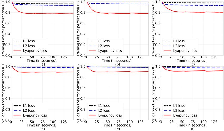
Experiments on larger datasets. In this section, we present results to demonstrate the performance
of our proposed algorithm on a larger dataset. We use the entire IMDB Wiki Faces Dataset Rothe
et al. (2015) with 0.5 million images for this experiment. Training dataset consists of ∼0.2 million
images and the test and validation set consists of ∼0.1 million images each. As described in the
previous section, a multi-layer perceptron is trained to predict the age from the image of a face. The
MLP is trained for 100 epochs with learning rate 0.0005 for all three loss functions and with α = 0.7
for Lyapunov loss function. From Figure 4 and Table 3, we can see that our proposed algorithm
achieves similar generalization / testing rmse (Root mean square error) as L1 and L2 baselines
while providing finite time convergence guarantees even on large datasets. The convergence time is
also within the theoretically derived upper bound.
Figure 4: Comparison of training convergence with respect to time for 0.5 million IMDB Wiki
dataset
Experiment Theoretical Upper Exp. Convergence Time Metric
Bound (in seconds) rmse
(in seconds) L1 L2 Lyap. L1 L2 Lyap.
IMDB Wiki 8.3e6 980.40 712.99 467.96 0.414 0.415 0.416
Table 3: rmse on IMDB Wiki test dataset for L1 , L2 and Lyapunov Loss function.
4 C ONCLUSION AND F UTURE W ORK
This paper studies the training of a deep neural network from control theory perspective. We pose
the supervised learning problem as a control problem by jointly designing loss function as Lyapunov
function and weight update as temporal derivative of the Lyapunov function. Control theory princi-
ples are then applied to provide guarantees on finite time convergence and settling time of the neural
network. Through experiments on benchmark datasets, our proposed method converges within the a
priori bounds derived from theory. It is also observed that in some cases our method enforces faster
convergence as compared to standard L1 and L2 loss functions. We also prove that our method is
robust to any perturbations in the input and convergence guarantees still hold true. The given a pri-
ori guarantees for the convergence time is a desirable result for training networks that are extremely
difficult to converge, specifically in Reinforcement Learning. A future scope of this work may be to
convert the continuous time analysis framework to discrete time. This study introduces a novel per-
spective of viewing neural networks as control systems and opens up the field of machine learning
research to a plethora of new results that can be derived from control theory.
9Under review as a conference paper at ICLR 2021
R EFERENCES
Zeyuan Allen-Zhu, Yuanzhi Li, and Zhao Song. On the convergence rate of training recurrent neural
networks. In Advances in Neural Information Processing Systems, pp. 6673–6685, 2019.
Sanjeev Arora, Nadav Cohen, Noah Golowich, and Wei Hu. A convergence analysis of gradient
descent for deep linear neural networks. arXiv preprint arXiv:1810.02281, 2018.
S.P. Bhat and D.S. Bernstein. Finite-Time Stability of Continuous Autonomous Systems. SIAM
Journal of Control and Optimization, 38(3):751–766, 2000.
Christopher M. Bishop. Neural Networks for Pattern Recognition. OXFORD University Press,
1995.
Simon S Du, Jason D Lee, Haochuan Li, Liwei Wang, and Xiyu Zhai. Gradient descent finds global
minima of deep neural networks. arXiv preprint arXiv:1811.03804, 2018.
Dheeru Dua and Casey Graff. UCI machine learning repository, 2017. URL http://archive.
ics.uci.edu/ml.
Dongsheng Guo, Chenfu Yi, and Yunong Zhang. Zhang neural network versus gradient-based neural
network for time-varying linear matrix equation solving. Neurocomputing, 74(17):3708–3712,
2011.
Harsh Gupta, R Srikant, and Lei Ying. Finite-time performance bounds and adaptive learning rate
selection for two time-scale reinforcement learning. In Advances in Neural Information Process-
ing Systems, pp. 4706–4715, 2019.
Eldad Haber and Lars Ruthotto. Stable architectures for deep neural networks. Inverse Problems,
34(1):014004, 2017.
David Harrison Jr and Daniel L Rubinfeld. Hedonic housing prices and the demand for clean air.
1978.
Arthur Jacot, Franck Gabriel, and Clément Hongler. Neural tangent kernel: Convergence and gen-
eralization in neural networks. In Advances in neural information processing systems, pp. 8571–
8580, 2018.
Maxim Kaledin, Eric Moulines, Alexey Naumov, Vladislav Tadic, and Hoi-To Wai. Finite time
analysis of linear two-timescale stochastic approximation with markovian noise. arXiv preprint
arXiv:2002.01268, 2020.
Yann LeCun, D Touresky, G Hinton, and T Sejnowski. A theoretical framework for back-
propagation. In Proceedings of the 1988 connectionist models summer school, volume 1, pp.
21–28. CMU, Pittsburgh, Pa: Morgan Kaufmann, 1988.
Shuai Li, Sanfeng Chen, and Bo Liu. Accelerating a recurrent neural network to finite-time conver-
gence for solving time-varying sylvester equation by using a sign-bi-power activation function.
Neural processing letters, 37(2):189–205, 2013.
Yuanzhi Li and Yang Yuan. Convergence analysis of two-layer neural networks with relu activation.
In Advances in neural information processing systems, pp. 597–607, 2017.
Guan-Horng Liu and Evangelos A Theodorou. Deep learning theory review: An optimal control
and dynamical systems perspective. arXiv preprint arXiv:1908.10920, 2019.
Yury Orlov. Finite-Time Stability and Robust Control Synthesis of Uncertain Switched Systems.
SIAM Journal of Control and Optimization, 43(4):1253–1271, 2005.
Rasmus Rothe, Radu Timofte, and Luc Van Gool. Dex: Deep expectation of apparent age from
a single image. In IEEE International Conference on Computer Vision Workshops (ICCVW),
December 2015.
Andrew M Saxe, James L McClelland, and Surya Ganguli. Exact solutions to the nonlinear dynam-
ics of learning in deep linear neural networks. arXiv preprint arXiv:1312.6120, 2013.
10Under review as a conference paper at ICLR 2021
Gang Wang, Bingcong Li, and Georgios B Giannakis. A multistep lyapunov approach for finite-time
analysis of biased stochastic approximation. arXiv preprint arXiv:1909.04299, 2019.
Lin Xiao. Accelerating a recurrent neural network to finite-time convergence using a new design
formula and its application to time-varying matrix square root. Journal of the Franklin Institute,
354(13):5667–5677, 2017.
Bin Xu, Chenguang Yang, and Zhongke Shi. Reinforcement learning output feedback nn control
using deterministic learning technique. IEEE Transactions on Neural Networks and Learning
Systems, 25(3):635–641, 2013.
Yunong Zhang, Danchi Jiang, and Jun Wang. A recurrent neural network for solving sylvester
equation with time-varying coefficients. IEEE Transactions on Neural Networks, 13(5):1053–
1063, 2002.
A A PPENDIX
A.1 I MPACT OF α ON TRAINING
The case when α = 0, as depicted in Figure 5, raises continuity issues.
Figure 5: Depiction of the numerical instability observed when we take α = 0. Effectively, at this
point, the loss function contains a discontinuous signum function.
Consider the left and right limits of the function f (%) = |%|α sign(%), where % = δj zi as appearing
in (15). It can be seen that lim%→0− f (%) = lim%→0+ f (%) = 0 for α ∈ (0, 1). However, for α = 0,
lim%→0− f (%) = −1 and lim%→0+ f (%) = 1. It should be noted that function f (%) is non-Lipschitz
since ∂f /∂% tends to infinity in the limit % → 0. We agree that α = 0 reduces the loss function to
L1 loss, but the control update becomes purely discontinuous due to the presence of f (%) in (15).
We do not deal with this case for the reasons of continuity as mentioned in the main paper.
A.2 E XPERIMENTS
A.2.1 E XPERIMENTAL S ETUP
For our experiments, we use the NVIDIA GEFORCE GTX1080Ti GPU card with 12GB RAM, 4-
core CPU with 32GB of RAM for training. The training code is in Python. All networks are trained
on data with an 80% − 20% train data-test data split.
11Under review as a conference paper at ICLR 2021
A.2.2 C ONVERGENCE EXPERIMENTS ON S INGLE N EURON
In this experiment, we perform binary classification on the Iris dataset (Dua & Graff (2017)) as a
representative example of single neuron case presented in Section 2.1.
Figure 6: Comparison of convergence with respect to time for a single neuron trained on the Iris
dataset. We convert the problem into a binary classification problem by considering only two of the
three output classes. All networks are trained for 2100 epochs with 80 training examples and 20 test
examples, α = 0.8, learning rate / k = 0.01
From the Figure 6, we can clearly see that Lyapunov loss function with control weight update con-
verges much faster towards zero as compared to L1 and L2 loss with standard gradient descent
weight update. This shows that explicitly adding a control weight update (15) that drives the loss
towards zero is helpful in reaching convergence faster.
A.2.3 B OSTON H OUSING DATASET EXPERIMENT WITH PERTURBATIONS
The Boston Housing Dataset predicts the price of houses in various areas of Boston Mass, given
14 different relevant attributes, like per capita crime rate and pupil-teacher ratio by town. The 506
examples in the data are divided into a 80-20 training-test split to give us 505 training examples and
101 test examples respectively. We consider three cases here, M = 0.1, M = 0.2 ,and M = 0.3.
Table 4 presents the theoretical upper bounds for the proposed Lyapunov function’s settling time
and experimental results for the training conducted for different upper bounds assumed for the input
perturbation. We observe that the settling time for the proposed Lyapunov function is similar to the
one observed for L2 loss function whereas it performs way better than the L1 loss function.
Experiment Theoretical Upper Exp. Convergence Time Metric
for MLP case Bound to within 10e-9 (in seconds) rmse
on Boston (in seconds) L1 L2 Lyap. L1 L2 Lyap.
dataset
M = 0.1 ∼ 1.97e11 1277.66 906.61 755.59 0.095 0.145 0.092
M = 0.2 ∼ 5.67e10 1297.11 1097.62 914.78 0.096 0.146 0.093
M = 0.3 ∼ 2.73e10 1290.48 1197.53 998.05 0.093 0.147 0.101
Table 4: Settling time in seconds for different values of the upper bound on additive input perturba-
tions, M for the multi layer perceptron case on Boston Housing dataset. We compare the time taken
for convergence by three different loss functions, L1 , L2 and Lyapunov Loss function. The training
conditions were similar for individual cases in the experiment.
12Under review as a conference paper at ICLR 2021
A.2.4 IMDB W IKI FACES E XPERIMENT ON PERTURBATIONS
Figure 7: Pictorial representation of the effect of random additive noise with an upper bound of 0.2
on IMDB Wiki Faces Dataset. In this experiment, we work with monochrome images for the sake
of simplicity.
Figure 7 shows us how the noise affects the training images. We take the specific case where M =
0.2. We can clearly observe that the images obtained after adding input perturbations happens to be
quite noisy. Figure 8 and Figure 9 show that even when inputs are perturbed, our proposed method
converges in finite time.
Figure 8: Comparison of training loss convergence with respect to time for different values of input
perturbations, ∆x for a multi-layer perceptron trained on the IMDB Wiki Faces dataset. The a priori
upper bound on input perturbations are as follows: (a) ∆x = 0.1, (b) ∆x = 0.2, (c)∆x = 0.3, (d)
∆x = 0.4, (e) ∆x = 0.5, and (f) ∆x = 1.2.
13Under review as a conference paper at ICLR 2021
Figure 9: Comparison of test loss convergence with respect to time for different values of input
perturbations, ∆x for a multi-layer perceptron trained on the IMDB Wiki Faces dataset.The a priori
upper bound on input perturbations are as follows: (a) ∆x = 0.1, (b) ∆x = 0.2, (c)∆x = 0.3, (d)
∆x = 0.4, (e) ∆x = 0.5, and (f) ∆x = 1.2.
14You can also read