Evaluating Pose Estimation Methods for Stereo Visual Odometry on Robots
←
→
Page content transcription
If your browser does not render page correctly, please read the page content below
Carnegie Mellon University
Research Showcase @ CMU
Robotics Institute                                                                                           School of Computer Science

8-2010

Evaluating Pose Estimation Methods for Stereo
Visual Odometry on Robots
Hatem Alismail
Carnegie Mellon University

Brett Browning
Carnegie Mellon University

M. Bernardine Dias
Carnegie Mellon University

Follow this and additional works at: http://repository.cmu.edu/robotics
     Part of the Robotics Commons

Published In
proceedings of the 11th International Conference on Intelligent Autonomous Systems (IAS-11).

This Conference Proceeding is brought to you for free and open access by the School of Computer Science at Research Showcase @ CMU. It has been
accepted for inclusion in Robotics Institute by an authorized administrator of Research Showcase @ CMU. For more information, please contact
research-showcase@andrew.cmu.edu.
Evaluating Pose Estimation Methods for
    Stereo Visual Odometry on Robots1
           Hatem ALISMAIL a , Brett BROWNING a and M. Bernardine DIAS a
  a
      Robotics Institute, Carnegie Mellon University, 5000 Forbes Avenue, Pittsburgh PA
          15213, USA. E-mail:{halismai,brettb,mbdias}@cs.cmu.edu
      B. Browning and M.B. Dias have split appointments with Carnegie Mellon Qatar,
                                   Education City, Qatar;

             Abstract. Structure-From-Motion (SFM) methods, using stereo data, are among
             the best performing algorithms for motion estimation from video imagery, or visual
             odometry. Critical to the success of SFM methods is the quality of the initial pose
             estimation algorithm from feature correspondences. In this work, we evaluate the
             performance of pose estimation algorithms commonly used in SFM visual odom-
             etry. We consider two classes of techniques to develop the initial pose estimate:
             Absolute Orientation (AO) methods, and Perspective-n-Point (PnP) methods. To
             date, there has not been a comparative study of their performance on robot visual
             odometry tasks. We undertake such a study to measure the accuracy, repeatability,
             and robustness of these techniques for vehicles moving in indoor environments and
             in outdoor suburban roadways. Our results show that PnP methods outperform AO
             methods, with P3P being the best performing algorithm. This is particularly true
             when stereo triangulation uncertainty is high due to a wide Field of View lens and
             small stereo-rig baseline.

             Keywords. Pose estimation, Visual odometry, PnP, Absolute orientation

Introduction

Visual Odometry (VO) is the problem of estimating camera motion using video imagery.
This problem must be solved if we are to create easily deployable mechanisms that are
not dependent on GPS coverage for positioning and do not need expensive Inertial Nav-
igation Systems (INSs). The low cost, small size, lower power needs, and high infor-
mation content of modern cameras make them attractive sensors to address this prob-
lem. There is a rich variety of approaches to VO including state estimation methods
such as Kalman filters [9,1] and particle filters [2], as well as Structure-From-Motion
(SFM) [12,17]. SFM methods are generally more scalable and more robust, especially
when using stereo as it resolves scale ambiguity. In this work, we are interested in evalu-
ating the performance of initial pose estimation algorithms that could be used in the SFM
stereo VO, as they are crucial to the success of the algorithm.
   1 The work for this paper was funded by the Qatar Foundation for Education, Science and Community

Development. The statements made herein are solely the responsibility of the authors and do not reflect any
official position by the Qatar Foundation or Carnegie Mellon University.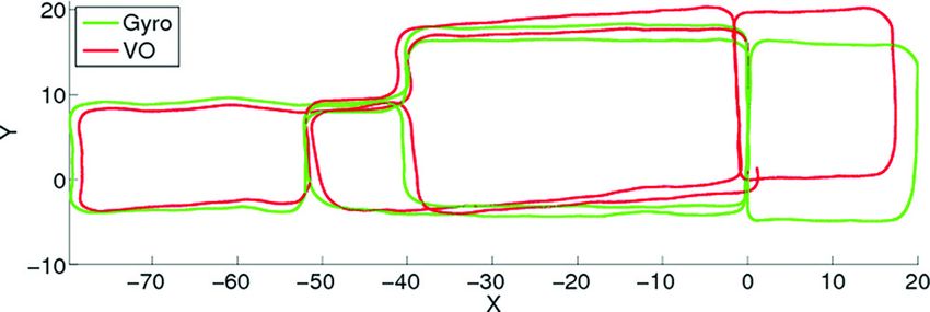
In the SFM approach to stereo VO [17,12], there are a number of design choices
that impact overall system performance. A core subset of these choices include how
to: detect local features, establish feature correspondences between frames, estimate an
initial pose, and refine that pose to reduce error accumulation. Empirical studies [20,
14] on refinement strategies and feature detection have provided a wealth of practical
knowledge for informing these choices. However, there have been few comparisons on
methods to initially estimate the pose prior to refinement.
     Given that refinement is only guaranteed to find a local optima, the accuracy and
reliability of pose estimation is crucial to the overall VO result. We undertake an em-
pirical study across the two major classes of techniques: Absolute Orientation meth-
ods (AO) and Perspective-n-points methods (PnP). AO methods estimate the pose of
the camera from 3D3D correspondences [8], while PnP methods use 2D3D correspon-
dences [3,11,18]. Our results show that PnP methods outperform AO methods in indoor
and outdoor environments with P3P being the best performing algorithm.

1. Stereo-based Visual Odometry Pipeline

To understand the role of initial pose estimation, we first describe the larger VO pipeline
in the theme of [17,12]. We start with the assumption of rigid 3D points X in the world
that are imaged by a calibrated stereo camera moving through a sequence of poses. Each
point, represented as a homogeneous 4-vector, is observed in the left image of an ideal
pinhole stereo camera on the nth frame as: xnL = K [Rn T n ] X. The goal of stereo VO
is to use these observed points, tracked over multiple frames, to estimate each 6 DOF
stereo pair camera pose: with rotation Rn and translation T n in the nth frame.
     For a calibrated stereo-rig, we can then determine the 3D location relative to the
camera (Y n ) of these detected features by matching features between the left (xnL )
and right images (xnR ) and performing stereo triangulation. By tracking features across
frames, say in the left image, we can use the sequence of correspondences to form an
initial estimate of the camera poses. The choice of whether to use the 2D information
measured directly in each frame, or the 3D information inferred through triangulation
determines the class of the pose estimation technique.
     Due to errors in triangulation, or errors in data association when matching features,
the initial pose estimation process must be made robust to gross outliers. The RANSAC
algorithm [3] and its variants have become very popular as an outlier detection scheme
for vision problems. RANSAC repeatedly samples k points to estimates the model and
outliers according to that model. The smaller the k is, the less iterations of RANSAC are
required to reach a desired confidence level. Refinement via techniques such as Sparse
Bundle Adjustment (SBA) [14,22], can then be used to polish the solution (e.g. [12]).
     In the next section, we describe a range of algorithms, which we then empirically
compare in the remainder of the paper.

2. Pose Estimation Algorithms

We group initial pose estimation methods into AO and PnP techniques. AO techniques
register estimated 3D world points to estimated 3D points in the camera frame, while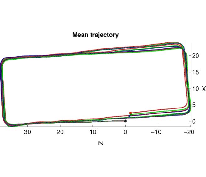
PnP techniques estimate pose from 3D world points and their 2D image projections.
Next, we briefly review the AO and PnP algorithms that we will evaluate.

2.1. Absolute Orientation

Given N 3D points X in Euclidean coordinate frame A and their corresponding 3D
locations Y in transformed frame B where X = RY + T + ,  is a noise term, the AO
problem is to estimate the unknown rotation and translation.2 Typically, noise is assumed
to be isotropic Gaussian, leading to a MLE formulation.
                                                   N
                                                   X
                            R∗ , T ∗ = argmin            ||Xi − (RYi + T )||2 .                              (1)
                                            R,T      i
A common step in many algorithm is decoupling the parameters by centering each of
the point sets about their centroids. This allows us to first focus on the Procrustes align-
ment problem, where one needs to solve for the rotation that best aligns the point sets.
A comparison of four major AO methods have demonstrated that SVD and quaternion
techniques
         PN produce the best results [13]. Here we use the SVD technique [23]. Define
H = N1 i (Yi − Ȳ )(Xi − X̄)T , where X̄ and Ȳ are the centroids of each point set.
Write the SVD of H as H = U SV T , then the optimal least squares rotation is given by
R∗ = V T GU , where G = diag(1, 1, det(U ) det(V )). The translation is then recovered
as: T ∗ = X̄ − R∗ Ȳ .
     This technique requires at least three non-colinear points to produce a solution. Thus,
a RANSAC version must sample at least 3 points per iteration. When data is not equally
accurate, a weighted version of this rule can also be derived3 .

                             Figure 1. Canonical depiction of the P 3P problem.

2.2. Perspective-N-Points

Given N 3D points X in coordinate frame A, and their 2D projections x in a calibrated
camera K, the PnP problem is to estimate the camera’s pose R and T relative to A.
We start with considering the case where N = 3 (shown in Figure 1). The solution to
this problem is to first solve for the depths along each ray and then perform an absolute
orientation step to solve for the camera pose. Following [5], we note that Si = ||Xi − C||
  2 Absolute orientation is usually derived for a similarity transform involving an isotropic scaling by s. Here,

we are primarily interested in Euclidean transforms where s = 1.
  3 Each point is weighted inversely proportional to its depth. If weights are normalized
                                                                                              PN
                                                                                                 i wi = 1, then
      1 PN                             T                1 PN
H= N       i  w i (Y i − Y
                         b )(X i −  X)
                                     b   ,where  Xb =   N     i  w i Xi is the weighed centroid of the point set.
is the unknown depth of point i from the camera center in the camera frame, while
dij = ||Xi − Xj || is the known inter-point distance obtained from stereo in the world
frame. The viewing ray for each points is ri = K −1 xi which is known and can be used
to calculate the angle between each pair of rays: cos θij = riT rj / (||ri ||||rj ||). Taken
together, we can form a series of polynomials in Si using the cosine rule:
d2ij = Si2 + Sj2 − 2Si Sj (cos θij ), for i, j ∈ {(1, 2), (1, 3), (2, 3)}. (2)
This polynomial system of equations can then be solved in a variety of ways to find the
unknown depths. In the original P3P, we solve for one of the unknown depths, say Si , by
eliminating each of the other depths from Eqn. (2), leading to an 8th degree polynomial
consisting of all even powers of Si . Substituting u = Si2 , as the depth must be strictly
positive, leads to a quartic polynomial that has up to four solutions.
G(u) = α4 u4 + α3 u3 + α2 u2 + α1 u + α0 . (3)
Haralick et al. [5] provides an excellent review of a wealth of nonlinear algorithms
that have been developed to address this problem. We call this approach the original P3P.
Linear variations on PnP algorithms have been also proposed [11,18] as well as
more efficient nonlinear methods (for n ≥ 4) [4]. Linear approaches to the PnP problem
rely on well established linear algebra techniques and can be solved very efficiently. The
main advantage, however, is that for n > 3 linear methods guarantee a unique solution.
Next, we briefly describe other PnP algorithms (see [18,11] for details).
L-P3P: is a linear solution by [11] that uses the Bzeout-Cayley-Dixon method. A
5 × 5 matrix B can be constructed from the set of polynomials in Eqn. (2) whose entries
are linear in S12 , which can be written as: B(S12 ) = B0 + S12 B2 where B2 is invertible.
The null vector of Bv = 0 contains a solution if one exists. From this system we obtain
(B2−1 B0 + q1−2 I)v = 0, which is solved by the Eigen value decomposition.
L-P4P: An additional point resolves some of the ambiguity in the P 3P solution.
It is possible, however, to obtain multiple solutions using four points in some degener-
ate configurations [10,21]. However, a linear algorithm can be designed to guarantee a
unique solution [19,18,11].
P5P and Beyond: Linear solutions have been also developed for the case of five
points [18] and even six points. For more than six points we can obtain a solution using
a direct linear transform method (DLT) [7]. However, a model of n > 4 points might
not be feasible for real-time applications due to the large number of RANSAC iterations
required to achieve a desired confidence level and the greater number of sample points
required to achieve a solution at all.
EPnP: An alternative non-linear solution with a linear running time, called EPnP,
was proposed by [4]. The authors compared their results to an iterative motion estimation
algorithm developed by [15] and showed that the algorithm is comparable and more
efficient suggesting its use in real-time systems.
2.3. Summary
Table 1 summarizes the list of algorithms used in this work. In the next section we de-
scribe our visual odometry testbed that we use to evaluate the relative performance of
these algorithms on mobile robot visual odometry tasks.Table 1. Table of motion estimation algorithms used in this work
Abbrv Algorithm
AO Absolute Orientation [23]
o-P 3P The original P3P [3]
l-P 3P Linear 3 points [11]
l-P 4P Linear 4 points [11]
EP nP Efficient PnP [4] (we use n = 5)
3. Visual Odometry Testbed
We have developed a full VO system to act as a testbed for evaluating the performance
of each initial pose estimation technique. In selecting an algorithm consideration must
be given to speed, accuracy, resolution (i.e. sub-pixel or not), and robustness to blur,
lighting and viewpoint changes. We follow [17] and extract many Harris corners [6] and
rely on RANSAC to remove outliers. Unlike [17], we first employ Laplacian of Gaussian
(LoG) filtering (σ = 3), which empirically increases the number of useful features, and
sub-pixel refinement to improve the stereo triangulation accuracy.
For feature matching we use Zero-mean Normalized Cross Correlation (ZNCC) be-
tween the grayscale 121D feature descriptors extracted at sub-pixel positions via bi-
linear interpolation from the 11 × 11 patch around each keypoint. If Ii , Ij ∈ Rn are the
two n = 121 feature descriptors to be compared, then we pre-calculate
P the normalization
P 2
parameters for each descriptor [17]. That is, we calculate ai = I i , bi = Ii , and
−1/2
ci = nbi − a2i . The score then becomes:
ZNCC(Ii , Ij ) = ci cj (nIiT Ij − ai aj ), (4)
so that only the dot product IiT Ij
needs to be re-calculated for each paired comparison.
We use ZNCC for both stereo matching and for frame-to-frame tracking and use a win-
dow constraint to limit the number of candidates. For stereo matching the window is a
narrow patch around the epipolar line. We allow some vertical disparity (±1 pixel), and
a horizontal disparity of δx ∈ [0, 64]. For successive frame pairs we use a symmetric
search window with δx , δy ∈ [−64, 64].
To estimate the pose, we use one of the algorithms in Table 1 wrapped within
a RANSAC routine for robustness. For this work, we use the vanilla formulation of
RANSAC [3] and test for outliers using the reprojection error in Eqn. (5).
To refine the pose estimates we use SBA [22] as implemented by [14]. For com-
putational efficiency, we use a sliding window approach similar to [12]. In order to en-
sure a fair comparison between pose estimation algorithms and reduce any window size
effects, we use a sufficiently large window consisting of 20 frames. Motion parameters
are optimized at every frame, while a simultaneous structure and motion refinement is
performed every 5th frame to ensure a sufficient baseline to constrain structure. SBA is
used to minimize the reprojection error E in each image in the sequence:
X
E = min D(Mi Xj , xij )2 , (5)
Mi ,Xj
ij
where Mi = K [Ri Ti ] is a projection matrix at frame i composed of a fixed and known
intrinsic matrix K, Ri and Ti are outputs of the pose estimation step, xij is the observed
projection of the 3D point j at camera i and D(·) denotes the Euclidean distance.4. Experiments and Results
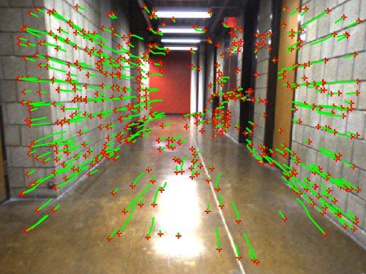
To provide a thorough evaluation of the motion estimation algorithms (shown in Table 1)
we use a range of indoor and outdoor datasets; an example is shown in Figure 2. Due
to space restrictions, we only show the results from some of these datasets and provide
summary statistics as appropriate.4
(a) (b)
Figure 2. Example of images from indoor and outdoor datasets
4.1. Indoor Datasets
We evaluated each of the pose estimation algorithms on a set of indoor datasets. These
datasets consist of a series of loops around an indoor environment with a Bumblebee2
stereo camera with a relatively wide FOV lens at 60◦ (f = 3.8mm). The camera was
mounted looking forward and titled towards the ground by ≈ 10◦ on a modified LAGR
robot that was manually operated. The robot was equipped with a high precision fiber
optic gyro, a lower quality IMU, and wheel encoders.
To evaluate the performance of each algorithm, we record statistics such as percent-
age of inliers, SBA errors, along with the estimated pose and structure. We evaluate the
performance of the algorithms by using these statistics or by performing direct compar-
isons to the ground truth estimates. The metrics we evaluated are:
• Repeatability We run the algorithm multiple times and evaluate the covariance
of the pose estimates at each time step. This gives a measure of how repeatable
the results are for the same dataset and feature correspondences. We compute
repeatability over multiple runs and record the average deviation from the mean.
• Loop Closure Measures the error between the start position and the end position
at the end of loops. We also express it as a percentage of distance travelled.
• SBA Reprojection Error We measure the reprojection error for the inliers both
prior to refinement (initial SBA err) and after refinement (final SBA err). This
indicates how good the initial pose estimate is and how much work SBA needs
to do to correct it. Error per run is in pixels and computed according to Eqn. (5).
Numbers shown in our results are averaged over multiple runs.
• Number of RANSAC iterations An indirect measure of computational perfor-
mance, it also indicates how easily RANSAC was able to find a solution.
• Percentage of inliers An indirect measure of the robustness of the technique.
4 See http://www.cs.cmu.edu/~halismai for downloadable datasets and additional results.Figure 3 shows graphically the repeatability results for the PnP algorithms, and Ta-
ble 2 summarizes the results obtained for each of the algorithms. Metrics for the weighted
and unweighted AO methods are not included because these techniques completely broke
down on the indoor data sets. Although these methods performed well on the outdoor
datasets, they failed to produce good path estimates on the indoor datasets. A possible
explanation is that the indoor datasets were collected with a shorter focal length, wider
FOV camera (60◦ instead of 43◦ used outdoors). The shorter focal length reduces the
range resolution for stereo triangulation which leads to greater deviation from the Gaus-
sian error model that AO implicitly relies on. Another possibility is that the distribution
of features in the images along with the range estimates is quite different for the indoor
and outdoor datasets. In either case, PnP techniques and P3P in particular appear to be
much more immune to these changes.
(a) (b)
(c) (d)
Figure 3. Algorithm repeatability results: Figures 3(a), 3(b) and 3(c) show standard deviation from the mean
of 10 runs for each of EP5P, o-P3P and l-P3P. Figure 3(d) shows the mean trajectory for the loop. Results are
shown in the camera coordinate system, where the Z-axis is aligned with the left camera principle axis.
Overall, the PnP algorithms do well on these datasets with the P3P algorithm clearly
dominating the performance. Based on these results, we further investigated the accuracy
of the P3P algorithm. On a more complex path, we compared the heading of the robot as
determined by VO and the heading as reported by the gyro. Figure 4 shows an overheadTable 2. Performance metrics for each algorithms in the indoor dataset. See text for units.
Alg Repeatability Loop Closure Initial SBA err Final SBA err Nr. Ransac % inliers
l-P3P 148.46 6.86 (1.50%) 16.45 13.41 29.10 0.58
o-P3P 179.50 6.29 (1.36%) 16.48 13.44 29.09 0.58
EP5P 199.00 7.87 (1.72%) 16.91 13.49 174.85 0.56
l-P4P 5.7×10⁵ 2.2×10³ (46.03%) 25.92 19.97 509.47 0.42
view of the robot trajectory using gyro heading estimates and wheel encoders versus pose
obtained from visual odometry.
Figure 4. Gyro/Robot distance 430.73m loop closure 0.3%, VO distance 424.3m loop closure 0.4%. Results
are shown in right-handed world coordinate system, +Z-axis point up.
4.2. Outdoor Datasets
We collected data on a range of outdoor datasets in two very different environments:
a flat desert environment with sparse vegetation and in a hilly temperate region with
dense vegetation. We report on the results for a 6.34km dataset in the desert region,
with vehicle speeds reaching 60km/h. The outdoor datasets were captured by mounting
the stereo head inside a car looking forward through the windscreen. A Garmin 18x-
5Hz GPS unit was used to capture WAAS corrected GPS at 5Hz, which was used for
ground truth. Although GPS with WAAS does not provide high resolution ground truth,
for sufficiently long vehicle paths the bounded error of the GPS is sufficient to bound the
odometry estimate error.
Table 3 shows some of the summary statitics. We do not show the repeatability,
and instead show the average error compared to the GPS pose interpolated to match the
time of the image capture. Overall, AO proved to be much more effective on the outdoor
datasets, but P3P still dominates the performance. While we do not show the detailed
results for the other algorithms, the qualitative results remain comparable.
Table 3. Performance metrics for the outdoor dataset. See text for units.
Alg. Loop Closure Initial SBA err Final SBA err Nr. Ransac % inliers
P3P 61 (1.1%) 69.29 59.49 96.70 0.41
AO 500 (8.1%) 88.74 61.73 2.55×10³ 0.30
Taken together, the results show that although AO approaches do reasonably well
on the outdoor datasets, they fail miserably on the indoor datasets even with a weighted
version of AO. PnP algorithms perform more reliably and accurately. In particular, P3P
dominates the other algorithms and should be the method of choice for stereo VO.5. Discussion
In this work, we have chosen to compare and evaluate the effect of initial pose estimation
algorithms on VO systems as this step is crucial to the reliability of the overall algorithm.
Closely related is the correctness and accuracy of feature matching across frames. While
we have used only a single feature type and a simple correlation window of fixed size to
search for correspondences, other approaches are possible.
Feature matching accuracy is very important and depends on feature types. Choice
of algorithms to extract features and descriptors depends on the environment. Konolige
et. al. [12] have shown that VO using CenSurE features and Harris corners have out-
performed SIFT for certain outdoor environments. Ultimately, however, the selection of
feature types depends on the environment and the amount of computation vs. quality of
features is a classic trade off. In this work, as we focused on the initial pose estimate,
we used Harris corners feature to hold constant the effect of the feature detector. Harris
corners are by far the most commonly used technique for feature detection due to its
speed and relatively good performance.
Inaccurate results from AO could intuitively be explained in light of the het-
eroscedastic nature of stereo triangulation error, especially for distal points relative to
FOV and baseline. The case of P3P being the most accurate is more interesting.
We believe that the superior performance of P3P relative to the rest of the algorithms
is attributed to the following reasons: (1) P3P, being a minimal solution, is more capable
of exploiting the projective constraints of the problem. (2) The PnP problem is nonlin-
ear at its core, linear PnP solutions for n > 3, while efficient and easy to implement,
their formulation does not account for the nonlinear nature of the problem. (3) While the
intent of adding more points is to resolve ambiguity and to add redundancy, this is not
necessarily what happens in real time VO, especially in unstructured environments. Lim-
ited computational power and the need for real time performance imposes two paradigms
for feature extraction for the same CPU cycles. One, is extracting a large number of
low quality features (e.g. corners). The other, is extracting a smaller number of features
but of higher quality (e.g. SIFT). The former approach will necessarily have a number
of incorrect feature matches, but the aim is to have a large enough number to estimate
motion. The latter approach might generate a very low number of features that are not
enough for reliable motion estimation (e.g. when image is saturated). In either case, the
algorithm with the lowest number of parameters has a higher chance of success. In a
RANSAC framework, the overall sample size required to obtain a solution in the worst
case is smaller for a model with a low number of parameters. Further, a model with a low
number of parameters has a higher probability of selecting a good subset of samples to
fit the model. This explains the reason that P3P performed better than EP5P.
6. Conclusions and Future Work
We have explored the use of Perspective-n-Points (PnP) techniques and Absolute Orien-
tation (AO) techniques for initially estimating the pose within a stereo visual odometry
system targeted towards mobile robot applications. We evaluated the performance of a
range of PnP and AO techniques for indoor and outdoor datasets and compared their
performance across a range of metrics. Overall, the P3P algorithm dominates the metricsfor both indoor and outdoor operation even when dealing with wider field of view cam-
eras and narrower stereo baselines. Our future work will include Maximum Likelihood
methods [9,16] and explore a broader range of datasets and environmental conditions.
Acknowledgments
The authors would like to thank members of the rCommerce group at the Robotics Insti-
tute, Balajee Kannan, Freddie Dias, Jimmy Bourne, Victor Marmol and Dominic Jonak
for their help with the robot hardware and data collection.
References
[1] A. J. Davison. Real-time simultaneous localisation and mapping with a single camera. In ICCV, 2003.
[2] E. Eade and T. Drummond. Scalable monocular slam. In CVPR, volume 1, pages 469–476, July 2006.
[3] M. A. Fischler and R. C. Bolles. Random sample consensus: a paradigm for model fitting with applica-
tions to image analysis and automated cartography. Commun. ACM, 24(6):381–395, June 1981.
[4] F.Moreno-Noguer, V.Lepetit, and P.Fua. Accurate non-iterative o(n) solution to the pnp problem. In
ICCV, Rio de Janeiro, Brazil, October 2007.
[5] R. M. Haralick, C.-N. Lee, K. Ottenberg, and M. Nölle. Review and analysis of solutions of the three
point perspective pose estimation problem. IJCV, 13(3):331–356, December 1994.
[6] C. Harris and M. Stephens. A combined corner and edge detection. In Proceedings of The Fourth Alvey
Vision Conference, pages 147–151, 1988.
[7] R. I. Hartley and A. Zisserman. Multiple View Geometry in Computer Vision. Cambridge University
Press, ISBN: 0521540518, second edition, 2004.
[8] B. K. Horn. Closed-form solution of absolute orientation using unit quaternions. Opt. Soc. Am., 1987.
[9] A. Howard. Real-time stereo visual odometry for autonomous ground vehicles. In IROS, 2008.
[10] Z. Y. Hu and F. C. Wu. A note on the number of solutions of the noncoplanar p4p problem. PAMI, 2002.
[11] M. Intell, Ameller, M. Quan, and L. Triggs. Camera pose revisited: New linear algorithms, 2002.
[12] K. Konolige, M. Agrawal, and J. Sola. Large-scale visual odometry for rough terrain, 2007.
[13] A. Lorusso, D. W. Eggert, and R. B. Fisher. A comparison of four algorithms for estimating 3-d rigid
transformations. In BMVC ’95 (Vol. 1), pages 237–246. BMVA Press, 1995.
[14] M. Lourakis and A. Argyros. The design and implementation of a generic sparse bundle adjustment soft-
ware package based on the levenberg-marquardt algorithm. Technical Report 340, Institute of Computer
Science - FORTH, Heraklion, Crete, Greece, Aug. 2004.
[15] C.-P. Lu, G. D. Hager, and E. Mjolsness. Fast and globally convergent pose estimation from video
images. PAMI, 22(6):610–622, 2000.
[16] M. Maimone, Y. Cheng, and L. Matthies. Two years of visual odometry on the mars exploration rovers.
Journal of Field Robotics, Special Issue on Space Robotics, 24, 2007.
[17] D. Nistér, O. Naroditsky, and J. Bergen. Visual odometry. In CVPR04, pages I: 652–659, 2004.
[18] L. Quan and Z. Lan. Linear n-point camera pose determination. PAMI, 21(8):774–780, 1999.
[19] G. Reid, J. Tang, and L. Zhi. A complete symbolic-numeric linear method for camera pose determina-
tion. In ISSAC ’03, pages 215–223. ACM, 2003.
[20] N. Sünderhauf, K. Konolige, S. Lacroix, P. Protzel, and T. U. Chemnitz. Visual odometry using sparse
bundle adjustment on an autonomous outdoor vehicle. In Tagungsband Autonome Mobile Systeme, 2005.
[21] J. Tang. Some necessary conditions on the number of solutions for the p4p problem. In LNCS, 2005.
[22] B. Triggs, P. F. Mclauchlan, R. I. Hartley, and A. W. Fitzgibbon. Bundle adjustment – a modern synthe-
sis. LNCS, 1883:298+, January 2000.
[23] S. Umeyama. Least-squares estimation of transformation parameters between two point patterns. PAMI,
13(4):376–380, 1991.You can also read