Constellation Queries over Big Data - SBBD
←
→
Page content transcription
If your browser does not render page correctly, please read the page content below
2018 SBC 33rd Brazilian Symposium on Databases (SBBD)                  August 25-26, 2018 - Rio de Janeiro, RJ, Brazil

                          Constellation Queries over Big Data
                    Fabio Porto1 , Amir Khatibi2 , João N. Rittmeyer1 ,
                 Eduardo Ogasawara3 , Patrick Valduriez4 , Dennis Shasha5
                                         1
                                             LNCC – Petropolis, RJ, Brazil
                                         2
                                             UFMG – Minas Gerais, Brazil
                                3
                                    CEFET-RJ – Rio de janeiro, RJ, Brazil
                                    4
                                        INRIA, Zenith, Montpellier, France
                     5
                         NYU, Computer Science Department, New York, USA
  {fporto,joaonr}@lncc.br, amir.khatibi.m@gmail.com,eogasawara@ieee.org

                  patrick.valduriez@inria.fr, shasha@courant.nyu.edu

      Abstract. A geometrical pattern is a set of points with all pairwise distances (or,
      more generally, relative distances) specified. Finding matches to such patterns
      has applications to spatial data in seismic, astronomical, and transportation
      contexts. Finding geometric patterns is a challenging problem as the potential
      number of sets of elements that compose shapes is exponentially large in the
      size of the dataset and the pattern. In this paper, we propose algorithms to find
      patterns in large data applications. Our methods combine quadtrees, matrix
      multiplication, and bucket join processing to discover sets of points that match
      a geometric pattern within some additive factor on the pairwise distances. Our
      distributed experiments show that the choice of composition algorithm (matrix
      multiplication or nested loops) depends on the freedom introduced in the query
      geometry through the distance additive factor. Three clearly identified blocks of
      threshold values guide the choice of the best composition algorithm.

      Resumo. Um padrão geométrico é definido por um conjunto de pontos e todos
      os pares de distâncias entre estes pontos. Encontrar casamentos de padrões
      geométricos em datasets tem aplicações na astronomia, na pesquisa sı́smica e
      no desenho de áreas urbanas. A solução do problema impõe um grande desafio,
      considerando-se o número exponencial de candidatos, potencialmente função
      do número de elementos no dataset e número de pontos na forma geométrica. O
      método aqui apresentado inclui: quadtrees,multiplicação de matrizes e junções
      espaciais para encontrar conjuntos de pontos que se aproximem do padrão
      fornecido, com um erro admissı́vel. Apresentamos uma implementação dis-
      tribuı́da reveladora de que a escolha do algoritmo (multiplicação de matrizes ou
      junções espaciais) depende da liberdade introduzida por um fator de erro adi-
      tivo na geometria do padrão. Identificamos três regiões baseadas nos valores
      de erro tolerados que determinam a escolha do algoritmo.

1. Introduction
The availability of large datasets in science, web and mobile applications enables new
interpretations of natural phenomena and human behavior. Consider the following use

                                                          85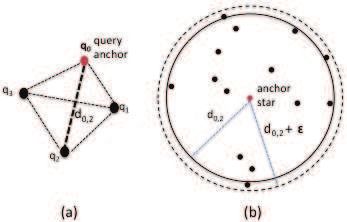
2018 SBC 33rd Brazilian Symposium on Databases (SBBD)        August 25-26, 2018 - Rio de Janeiro, RJ, Brazil

case: Scenario 1. An astronomy catalog is a table holding billions of sky objects from a
region of the sky, captured by telescopes. An astronomer may be interested in identifying
the effects of gravitational lensing in quasars, as predicted by Einstein’s General Theory
of Relativity [Einstein 2015]. According to this theory, massive objects like galaxies bend
light rays that travel near them just as a glass lens does. Due to this phenomenon, an earth
telescope would receive two or more virtual images of the lensed quasar leading to a
composed new object (Figure 1), such as the Einstein cross [Overbye 2015].

                Figure 1. Einstein Cross identification from astronomic catalogs

        In the scenario above, constellations, such as the Einstein cross, are obtained from
compositions of individual elements in large datasets in some spatial arrangement with
respect to one another. Thus, extracting constellations from large datasets entails match-
ing geometric pattern queries against sets of individual data observations, such that each
set obeys the geometric constraints expressed by the pattern query.
        Solving a constellation query in a big dataset is hard due to the sheer number
of possible compositions from billions of observations. In general, for a big dataset D
anda number k of elements in the pattern, an upper bound for candidate combinations
 |D|
  k
      is the number of ways to choose k items from D. This paper focuses primarily on
pure constellation queries (when all pairwise distances are specified up to an additive
factor). We develop parallel algorithms that reduce the number of possible candidate sets
by applying local and global constraints.
        The remainder of this paper is organized as follows. Section 2 formalizes the
constellation query problem. Section 3 presents our techniques to process constellation
queries. In section 4, we preset our algorithms. Section 5 discusses our experimental
environment and discusses the evaluation results, followed by section 6 that discusses
related work. Finally, section 7 concludes.

2. Problem Formulation
In this section, we introduce the problem of answering pure Constellation Queries on
a dataset of objects. A Dataset D defined as a set of elements (or objects) D =
{e1 , e2 , . . . , en }, in which each ei , 1 ≤ i ≤ n, is an element of a domain Dom. Fur-
thermore, ei =< atr1 , atr2 , . . . , atrm >, such that atrj (1 ≤ j ≤ m) is a value describing
a characteristic of ei .

                                                        86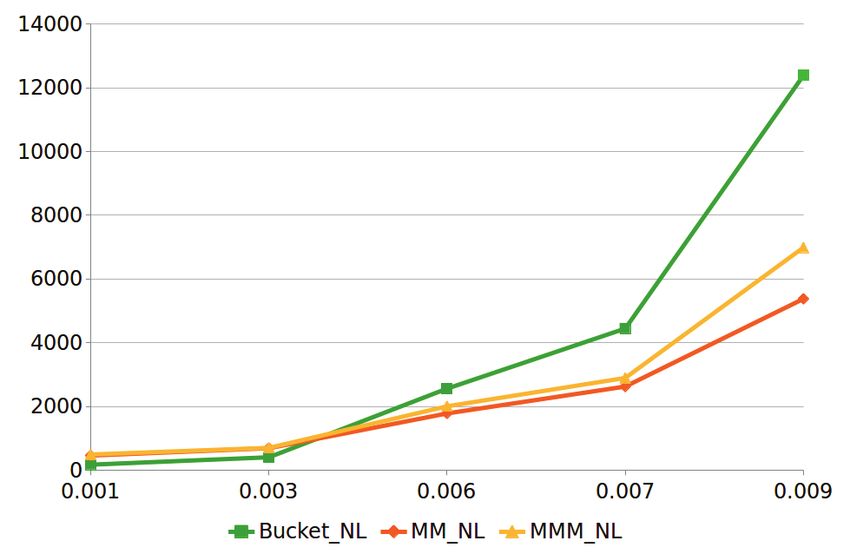
2018 SBC 33rd Brazilian Symposium on Databases (SBBD) August 25-26, 2018 - Rio de Janeiro, RJ, Brazil
A constellation query Qk = {q1 , q2 , . . . , qk } is (i) a sequence of k elements of do-
main Dom, (ii) the distances between the centroids of each pair of query elements that de-
fine the query shape and size with an additive allowable factor ǫ, and (iii) an element-wise
function f (e, q) that computes the similarity (e.g. in brightness at a certain wavelength)
between elements e and q up to a threshold θ.
A sequence s of elements of length k in D property matches query Q if every
element s[i] in s satisfies f e(s[i], qi ) up to a threshold θ and for every i, j ≤ k: (i) the dis-
tance between elements s[i] and s[j] is within an additive factor ǫ of the distance between
qi and qj , which is referred to as distance match. The solutions obtained using property
match and distance match to solve a query Q are referred to as pure constellations.
3. Pure Constellation Queries
Applying pure constellation to find patterns such as the Einstein cross over an astronomy
catalog requires efficient query processing techniques as the catalog may hold billions of
sky objects.
In this context, efficiently answering pure constellation queries involves constrain-
ing the huge space of candidate sets (i.e. subsets of the catalog with the same number of
stars as the query).
The next sections describe in detail the query processing techniques.
3.1. Reducing Data Complexity using a Quadtree
A constellation query looks for patterns in large datasets, such as the 2MASS catalog.
Computing constellation queries involves matching each star to all neighboring stars with
respect to the distances in the query, a costly procedure in large catalogs. To reduce this
cost, we adopt a filtering process that eliminates space regions where solutions cannot
exist.
The filtering process is implemented on top of a quadtree [Samet 1990], con-
structed over the entire input dataset. The quadtree splits the 2-dimensional catalog space
into successively refined quadrangular regions.
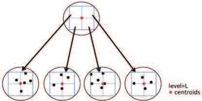
Figure 2. Quadtree node representation
A node in the tree is associated to a spatial quadrant. The geometric center of the
quadrant is the node centroid and is used as a representative for all stars located in that
quadrant, for initial distance matching evaluation. The quadtree data structure includes: a
root node, at level L = 0; a list of intermediary nodes, with level 1 ≤ L ≤ tree height −
87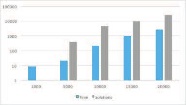
2018 SBC 33rd Brazilian Symposium on Databases (SBBD)        August 25-26, 2018 - Rio de Janeiro, RJ, Brazil

1; and leaf nodes. To avoid excessive memory usage, data about individual stars are stored
only in leaf nodes, Figure 2.
         The algorithm begins by determining the level of the quadtree Le at which the ǫ
error bound exceeds the diameter of the node. If we make the reasonable assumption that
ǫ is less than the minimum distance between elements in the query (minq), then at height
Le no two stars would be covered by a single quadtree node.
        Given a star s that will correspond to the centroid q0 of the pattern being matched,
the first step is to eliminate all parts of the quadtree that could not be relevant. The
algorithm finds the node at level Le containing s. That is called the query anchor node.
The algorithm finds the nodes that lie within a radius ρ of the query anchor node, where
ρ is the maximum distance plus the additive error bound ǫ between the centroid of the
query pattern and any other query element. As depicted in Figure 3, in (a) a query Q has
an anchor element q0 and the largest distance to the remaining query elements d0,2 . In
(b), a star is picked as an anchor and all neighboring stars within distance d0,2 + ǫ are
preliminary candidates for distance matching.

      Figure 3. (a) Pure constellation query with anchor and maximum distance (b)
      Neighboring elements of anchor element

        Next the algorithm determines for each pattern element qi , which stars are at dis-
tance dist(q0 , qi ) from s within an additive factor of ǫ. Such stars might correspond to qi in
the case where s corresponds to q0 . For each pair of nodes n1 and n2, where n1 contains
s and n2 may contain stars that correspond to qi for some i, the algorithm checks whether
the distance between the centroids of n1 and n2 matches dist(q0 , qi ), taking into account
both the diameter of the nodes and the error bound. This procedure filters out all node
pairs at that level for which no matching could possibly occur.
        If n2 has not been filtered out, then a simple test determines whether going one
level down the tree is cost effective as opposed to testing pairs of individual stars in the
two nodes. That test consists of determining whether any pair of children of n1 and n2
will be eliminated from consideration based on a distance test to the centroids of those
children. If so, then the algorithm goes down one level. The same matching procedure is
applied to the children nodes of n1 and n2 respectively. If not, then the stars for n1 and n2
are fetched and any star in n2 that lies within an ǫ additive bound of s is put into bucket
Bi .

                                                        88
2018 SBC 33rd Brazilian Symposium on Databases (SBBD) August 25-26, 2018 - Rio de Janeiro, RJ, Brazil
3.2. Composition algorithms
In this section, we discuss approaches to join the buckets produced by the filtering step.
As we will observe in section 5, composition algorithms are the most time consuming
operation in processing constellation queries. A given anchor node may generate buck-
ets containing thousands of elements. Thus, finding efficient composition algorithms is
critical to efficient overall processing.
3.2.1. Buckets Nested Loop (Bucket-NL)
An intuitive way to produce constellations for a given anchor element is by directly join-
ing the buckets of candidate elements considering the corresponding pairwise distances
between query elements as the join predicate. In this approach, each bucket is viewed
as a relation, having as a schema their spatial coordinates and an id, Bi (starid, ra, dec).
A solution is obtained whenever a tuple is produced having one neighbor element from
each bucket, such that the distances between each element in the solution distance-match
those among respective query elements, +/- ǫ. Bucket-NL assumes a nested loop algo-
rithm to traverse the buckets of candidate elements and checks for the distance predicates.
Thus, applying a distance-match constraint corresponds to applying a cyclic join among
all buckets in the bucket set followed by a filter among non-neighbors in the cycle. For
example, Bucket-NL would find pairs (t1, t2) where t1 is from Bi with and t2 from Bi+1
if dist(t1, t2) is within dist(pi , pi+1 ) +/- ǫ. Then given these pairs for buckets 1 and 2,
buckets 2 and 3, buckets 3 and 4, etc, Bucket-NL will join these cyclically and then for
any k-tuple of stars s1, s2, ..., sk that survive the join, Bucket-NL will also check the
distances of non-neighboring stars (e.g. check that dist(s2,s5) = dist(p2 , p5 ) +/- ǫ).
3.2.2. Matrix Multiplication based approaches
The Matrix Multiplication (M M ) based approaches precede the basic Bucket N L algo-
rithm by filtering out candidate elements. Here are the details: recall that bucket Bi holds
elements for the candidate anchor that correspond to dist(q0 , qi ) +/- ǫ. Compute the ma-
trices: M 1(B1 , B2 ), M 2(B2 , B3 ), M 3(B3 , B1 ) where M i(Bi , Bi+1 ) has a 1 in location j,
k if the jth star in Bi and the kth star in Bi+1 is within dist(pi , pi+1 ) +/- ǫ. The product of
matrices indicates the possible existence of solutions for a given anchor element, as long
as the resulting matrix contains at least a one in its diagonal. The MM approach can be
implemented with fast matrix multiplication algorithms [R. Bank 1993][U. Zwick 2005]
and enables quick elimination of unproductive bucket elements.
3.2.3. MMM Filtering
Matrix multiplication may be applied multiple times to eliminate stars that cannot be part
of any join. The idea is to apply k matrix multiplications, each with a sequence of matrices
starting with a different matrix (i.e. a Bi bucket appears in the first and last matrices of a
sequence, for 1 ≤ i ≤ k). The resulting matrix diagonal cells having zeros indicate that
the corresponding element is not part of any solution and can be eliminated. For example,
for buckets B1 , B2 , B3 and matrices M 1(B1 , B2 ), M 2(B2 , B3 ), M 3(B3 , B1 ), we would
892018 SBC 33rd Brazilian Symposium on Databases (SBBD) August 25-26, 2018 - Rio de Janeiro, RJ, Brazil
run < M 1 · M 2 · M 3 >; < M 2 · M 3 · M 1 > and < M 3 · M 1 · M 2 >. For the
multiplication starting with say M 1, elements in bucket B1 with zeros in the resulting
matrix diagonal are deleted from B1 , reducing the size of the full join.
3.2.4. Matrix Multiplication Compositions
The matrix multiplication filtering is coupled with a composition algorithm leading to
M M Composition algorithms. The choices explore the tradeoff between filtering more
by applying the MMM filtering strategy or not.
The MMM NL strategy uses the MMM filtering strategy to identify the elements
of each bucket that do not contribute to any solutions and can be eliminated from their
respective buckets. Next, the strategy applies Bucket NL to join the buckets with elements
that do contribute to solutions.
The MM NL considers a single bucket ordering with the anchor node bucket at the
head of the list. Thus, once the multiplication has been applied, elements in the anchor
node bucket that appear with zero in the resulting matrix diagonal are filtered out from
its bucket. Next, the strategy applies Bucket NL to join the buckets with anchor elements
that do contribute to solutions.
4. Algorithms for Pure Constellation Queries
To compute Pure Constellation Queries, the overall algorithm implements property
matching and finds matching pairs, whereas the composition algorithms implement dis-
tance matching as discussed above.
4.1. Main Algorithm
The Constellation Algorithm depicts the essential steps needed to process a Constellation
query. The main function is called ExecuteQuery. It receives as input a query q, dataset
D, element predicate f e, similarity threshold θ, and error bound ǫ. At step 1, a quadtree
entry level Le is computed. Next, a quadtree qt is built covering all elements in D and
having height Le . Figure 2.a illustrates a typical quadtree built on top of heterogeneously
distributed spatial data. The quadtree nodes at level Le become the representatives of stars
for initial distance matching. Considering the list of nodes at level Le , an iteration picks
each node, takes it as an anchor node, and searches qt to find neighbors. The geometric
centroid of the node quadrant is used as a reference to the node position and neighborhood
computation. Next, each pair (anchor node, neighbor) is evaluated for distance matching
against one of the query pairs: (query anchor, query element) and additive factor ǫ. Match-
ing nodes contribute with stars for distance matching or can be further split to eliminate
non-matching children nodes. Matching stars are placed in a bucket holding matches for
the corresponding query element.
The Compose Function, applies a composition algorithm, described in the previ-
ous section, between buckets B = {B1 , B2 , . . . , Bk }, for q.size = k + 1, to see which
k+1-tuples match the pure constellation query. The composition algorithm builds a query
execution plan to join buckets in B. The distance matching of elements in buckets Bi and
Bj , i 6= j, and i, j 6= anchor, is applied by checking their pairwise distances +/- ǫ, with
respect to the corresponding distances between qi and qj , in q.
902018 SBC 33rd Brazilian Symposium on Databases (SBBD) August 25-26, 2018 - Rio de Janeiro, RJ, Brazil
The choice between running Bucket NL or a MM filtering algorithm to implement
element composition, as our experiments in section 5 will show, is related to the size
of the partial join buckets. For dense datasets and queries with an error bound close to
the average distance among stars, lots of candidate pairs are produced and MM filtering
improves composition performance, see Figure 4.b.
5. Experimental Evaluation
In this section, we start by presenting our experimental setup. Next, we assess the different
components of our implementation for Constellation Queries.
5.1. Set Up
5.1.1. Dataset Configuration
The experiments focus on the Einstein cross constellation query and are based on
an astronomy catalog dataset obtained from the Sloan Digital Sky Survey (SDSS), a
seismic dataset, as well as synthetic datasets. The SDSS catalog, published as part
of the data release DR12, was downloaded from the project website link (http :
//skyserver.sdss.org/CasJobs/).
We consider a projection of the dataset including attributes (objID, ra, dec, u, g, r, i, z).
The extracted dataset has a size of 800 MB containing around 6.7 million sky objects.
The submitted query to obtain this dataset follows:
Select objID, ra, dec, u, g, r, i, z
From PhotoObjAll into MyTable
From the downloaded dataset, some subsets were extracted to produce datasets
of different size. Additionally, in order to simulate very dense regions of the sky, we
built synthetic datasets with: 1000, 5000, 10000, 15000, and 20000 stars. The synthetic
dataset includes millions of scaled solutions in a very dense region. Each solution is a
multiplicative factor from a base query solution chosen uniformly within an interval of
scale factors s = [1.00000001, 1.0000009].
5.1.2. Calibration
We calibrated constellation query techniques using the SDSS dataset described above and
a 3D seismic dataset from a region on the North Sea: Netherlands Offshore F3 Block
Complete 1 . The procedure aimed at finding the Einstein Cross in the astronomy catalog
and a seismic dome within the North Sea dataset, using our constellation query answering
techniques. In both cases, the techniques succeeded in spotting the right structures among
billions of candidates.
5.1.3. Computing Environment
The Constellation Query processing is implemented as an Apache Spark dataflow running
on a shared nothing cluster. The Petrus.lncc.br cluster is composed of 6 DELL PE R530
1
https://opendtect.org/osr/pmwiki.php
912018 SBC 33rd Brazilian Symposium on Databases (SBBD) August 25-26, 2018 - Rio de Janeiro, RJ, Brazil
servers running CENTOS v. 7.2, kernel version 3.10.0327.13.1
.el7.x86 64. Each cluster node includes a 2 Intel Xeon E5-2630 V3 2.4GHz processors,
with 8 cores each, 96 GB of RAM memory, 20MB cache and 2 TB of hard disk. We are
running Hadoop/HDFS v2.7.3, Spark v2.0.0 and Python v2.6. Spark was configured with
50 executors each running with 5GB of RAM memory and 1 core. The driver module was
configured with 80GB of RAM memory. The implementation builds the quadtree at the
master node, at the driver module, and distributes the list of nodes at the tree entry level.
Each worker node then runs the property matching and distance matching algorithms.
Finally, answers are collected in a single solution file.
5.2. The Effectiveness of the Descent Tree algorithm
The quadtree structure enables reducing the cost of constellation query processing by re-
stricting composition computation to stars in pairs of nodes whose spatial quadrants match
in distance. Selected matching pair nodes are evaluated for further splitting, according to
cost model. In this section, we investigate the efficiency of the algorithm. We compare the
cost of evaluating the stars matching at the tree entry level with one that descends based
on the cost model.
We ran the buildQuadtree function with dense datasets and measured the differ-
ence in elapsed-time in both scenarios. In terms of number of comparisons for 1 million
stars, the cost model saves approximately 1.9x, leading to an order of magnitude on exe-
cution time savings.
5.3. Composition Algorithm Selection
In this section, we discuss the characteristics of the proposed composition algorithms.
In the first experiment a constellation query based on the Einstein cross elements is
run for each composition algorithm and their elapsed-times are compared. The elapsed-
time values correspond to the average of 10 runs measuring the maximum among all
parallel execution nodes in each run.
The geometric nature of constellation queries and the density of astronomical cat-
alogs make the distance additive factor ǫ a very important element in query definition. As
our experiments have shown, variations in this parameter may change a null result set to
one with million of solutions. The experiments evaluate two classes of composition algo-
rithms. In one class, we use the Bucket NL algorithm and, in the second one, we include
the adoption of various Matrix Multiplication filtering strategies.
The experiment results are depicted in Figures 4.a and 4.b. In these plots, the
horizontal axis presents different error tolerance values ǫ, while the vertical axis shows the
elapsed-time of solving the constellation query using one of the composition algorithms.
Figure 4.a shows basically two scenarios. For very small ǫ, ≤ 10−6 , the number of
candidate elements in buckets is close to zero, leading to a total of 32 anchor elements to
be selected and producing 52 candidate shapes. In this scenario, the choice of a compo-
sition algorithms is irrelevant, with a difference in elapsed-time of less than 10% among
them. It is important to observe, however, that such a very restrictive constraint may elim-
inate interesting sets of stars. Unless the user is quite certain about the actual shape of its
constellation, it is better to loosen the constraint.
922018 SBC 33rd Brazilian Symposium on Databases (SBBD) August 25-26, 2018 - Rio de Janeiro, RJ, Brazil
The last blocks of runs involving the composition algorithms in Figure 4.a shows
that the results are different when increasing ǫ by up to a factor of 100. Considering
ǫ = 2, 0 × 10−5 ,we obtain 522, 578 productive anchor elements and an average of close
to one element per bucket. The total number of candidate shapes rises to 12.6 million.
In this setting, Bucket N L is very fast, as it loops over very few elements in the buck-
ets to discover solutions. The overhead of computing matrix multiplication is high, so
Bucket N L is a clear winner. This scenario continues to hold up to ǫ = 2 × 10⁻⁴ , see
Figure 4.a. In this range, Bucket N L is faster than M M N L and M M M N L by 214%
and 240%, respectively.
Figure 4.b highlights the behavior of algorithms under additive error tolerance val-
ues. The flexibility introduced by ǫ = 6 × 10⁻³ generates 6.7 million productive anchor
elements and a total of 7.1 billion solutions, with average elements per bucket of 10. In
this scenario, eliminating non-productive anchor elements, close to 300, 000, by filtering
using matrix multiplication eliminates the need of computing nested loops over approxi-
mately 405 candidate elements in buckets. Thus, running fast matrix multiplication as a
pre-step to nested-loop becomes beneficial.
Figure 5 shows the point at which matrix multiplication becomes beneficial: when
ǫ = 6.0 × 10⁻³ matrix multiplication starts to efficiently filter out anchor nodes and so
the reduction in nested-loop time compensates for the cost of performing matrix multipli-
cation. The gains observed by running matrix multiplication algorithms as a pre-filtering
step before nested loop for ǫ in range 6 × 10⁻³ and 9 × 10⁻³ are up to 45.6% for MM NL
and 34.6% for MMM NL.
(a) (b)
Figure 4. Low Additive Error Tolerance ǫ (a) High Additive Error Tolerance ǫ (b)
Figures 5.a and 5.b zoom in on the Matrix Multiplication algorithms. The former
shows the results with thresholds not less than 1 × 10⁻³ . In this range, we can observe an
inversion in performance between M M N L and M M M N L. The inflexion point occurs
after ǫ ≥ 2 × 10⁻³ . Threshold values below the inflexion point include anchor nodes with
very few elements in buckets. In this scenario, computing multiple matrix multiplication
is very fast. Moreover, elements that appear with zeros in the resulting matrix diagonal
can be looked up in buckets and deleted, before the final nested-loop. The result is a
gain of up to 14% in elapsed-time with respect to M M N L. From the inflexion point
on, M atrix M ultiplication N L is the best choice with gains up to 30% with respect
to M M M N L. The selection among composition algorithms is summarized in Table 1,
932018 SBC 33rd Brazilian Symposium on Databases (SBBD) August 25-26, 2018 - Rio de Janeiro, RJ, Brazil
according to the results on the SDSS dataset.
Table 1. Composition Algorithms Selection
Best Choice
Threshold-Range Composition
Algorithm
≤ 0.003 Bucket N L
> 0.003 MM NL
Finally, the matrix multiplication MM algorithm is, as expected, a good choice for
existential constellation queries which ask whether any subset of the dataset matches the
query but does not ask to specify that subset. In this scenario, once the matrix multiplica-
tion indicates a resulting matrix diagonal with all zeros, the anchor element produces no
candidate shape and can be eliminated from the existential query result.
(a) (b)
Figure 5. Zoom In on Matrix Multiplication: large threshold (a) Zoom In on Matrix
Multiplication: low threshold (b)
5.4. Pure Constellation Scale-up
We investigated Pure CQ scale-up adopting the set of dense datasets (see section 5.1.1),
error bound epsilon = 4.4x10⁻⁶ and Bucket NL for the composition algorithm. The exe-
cution produced solutions of size: zero, 21, 221, 1015, and 2685. The run with 1000 stars
dataset produced zero solutions, which shows the relevance of tunning the error bound
for a given dataset and the restrictions imposed by Pure CQ. Apart from the runs with
the 15,000 stars dataset, the variations in time followed the increase in the number of
solutions.This indicates that non solutions are quickly discarded and the time is mostly
due to producing solutions. Figure 6 depicts the results, where time corresponds to the
elapsed-time in seconds of the parallel execution.
6. Related Work
Finding collections of objects having some metric relationship of interest is an area with
many applications. The problem has different names depending on the discipline, includ-
ing Object Identification [Singla and Domingos 2005], Graph Queries [Zou et al. 2011],
Pattern Matching and Pattern Recognition [Bishop 2006].
942018 SBC 33rd Brazilian Symposium on Databases (SBBD) August 25-26, 2018 - Rio de Janeiro, RJ, Brazil
Figure 6. Pure Constellation Scale-up
Pattern recognition research focuses on identifying patterns and regularities in data
[Bishop 2006]. Graphs are commonly used in pattern recognition due to their flexibility
in representing structural geometric and relational descriptions for concepts, such as pix-
els, predicates, and objects [Jolion 2001]. In this way, problems are commonly posed as
a graph query problem, such as subgraph search, shortest-path query, reachability veri-
fication, and pattern match. Among these, subgraph matching queries are related to our
work.
In a subgraph query, a query is a connected set of nodes and edges (which may
or may not be labeled). A match is a (usually non-induced) subgraph of a large graph
that is isomorphic to the query. While the literature in that field is vast [[Zou et al. 2009],
[Giugno and Shasha 2002]], the problem is fundamentally different, because there is no
notion of space (so data structures like quadtrees are useless) and there is no distance
notion of scale (the ǫ that plays such a big role for us).
Finally, constellation queries are a class of package queries (PQ), Brucato et al.
[Brucato et al. 2016].
7. Conclusion
In this paper, we introduce constellation queries, specified as a geometrical composition
of individual elements from a big dataset. We illustrate the application of Constellation
Queries in astronomy (e.g. Einstein crosses).
We have designed procedures to efficiently compute both pure Constellation
Queries. First, we reduce the space of possible candidate sets by associating to each
element in the dataset neighbors at a maximum distance, corresponding to the largest dis-
tance between any two elements in the query. Next, we filtered candidates yet further
into buckets through the use of a quadtree. Next, we used a bucket joining algorithm,
optionally preceded by a matrix multiplication filter to find solutions.
Our experiments execute on Spark, running on the neighboring dataset distributed
over HDFS. Our work shows that our filtering techniques having to do with quadtrees are
enormously beneficial, whereas matrix multiplication is beneficial only in high density
settings.
There are numerous opportunities for future work, especially in optimization for
higher dimensions.
952018 SBC 33rd Brazilian Symposium on Databases (SBBD) August 25-26, 2018 - Rio de Janeiro, RJ, Brazil
8. Acknowledgment
This research is partially funded by EU H2020 Program and MCTI/RNP-Brazil(HPC4e
Project - grant agreement number 689772), FAPERJ (MUSIC Project E36-2013) and
INRIA (SciDISC 2017), INRIA international chair, U.S. National Science Foundation
MCB-1158273, IOS-1139362 and MCB-1412232. This support is greatly appreciated.
References
Bishop, C. M. (2006). Pattern recognition and machine learning. Springer, page 7.
Brucato, M., Beltran, J. F., Abouzied, A., and Meliou, A. (2016). Scalable package
queries in relational database systems. Proc. VLDB Endow., 9(7):576–587. 00004.
Einstein, A. (2015). Relativity: The special and the general theory.
Giugno, R. and Shasha, D. (2002). GraphGrep: A fast and universal method for querying
graphs. In Proceedings - International Conference on Pattern Recognition, volume 16,
pages 112–115. 2 edition. 00125.
Jolion, J. (2001). Graph matching : what are we really talking about. Proceedings of the
3rd IAPR Workshop on Graph-Based Representations in Pattern Recognition.
Overbye, D. (2015). Astronomers observe supernova and find they’re watching reruns.
New York Times, USA.
R. Bank, C. D. (1993). Sparse matrix multiplication package (smmp). Advances in Com-
putational Mathematics, 1:127–137.
Samet, H. (1990). The Design and Analysis of Spatial Data Structures. Addison-Wesley.
Singla, P. and Domingos, P. (2005). Object identification with attribute-mediated depen-
dences. Proceedings of the 9th European conference on Principles and Practice of
Knowledge Discovery in Databases.
U. Zwick, R. Y. (2005). Fast sparse matrix multiplication. ACM Transactions on Algo-
rithms (TALG), 1:2–13.
Zou, L., Chen, L., and Özsu, M. T. (2009). Distance-join: Pattern Match Query in a Large
Graph Database. Proc. VLDB Endow., 2(1):886–897.
Zou, L., Chen, L., Özsu, M. T., and Zhao, D. (2011). Answering pattern match queries in
large graph databases via graph embedding. The VLDB Journal, 21:97–120.
96You can also read