Learning to Place New Objects
←
→
Page content transcription
If your browser does not render page correctly, please read the page content below
Learning to Place New Objects
Yun Jiang, Changxi Zheng, Marcus Lim and Ashutosh Saxena
Abstract— The ability to place objects in an environment is
an important skill for a personal robot. An object should not
only be placed stably, but should also be placed in its preferred
location/orientation. For instance, it is preferred that a plate
be inserted vertically into the slot of a dish-rack as compared
to being placed horizontally in it. Unstructured environments
such as homes have a large variety of object types as well as
of placing areas. Therefore our algorithms should be able to
handle placing new object types and new placing areas. These
reasons make placing a challenging manipulation task.
In this work, we propose using a supervised learning ap-
proach for finding good placements given point-clouds of the
object and the placing area. Our method combines the features
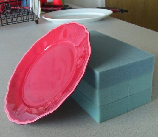
that capture support, stability and preferred configurations, Fig. 1: How to place an object depends on the shape of the object
and uses a shared sparsity structure in its the parameters. and the placing environment. For example, a plate could be placed
Even when neither the object nor the placing area is seen vertically in the dish rack (left), or placed slanted against a support
previously in the training set, our learning algorithm predicts (right). Furthermore, objects can also have a ‘preferred’ placing
good placements. In robotic experiments, our method enables configuration. E.g., in the dish rack above, the preferred placement
the robot to stably place known objects with a 98% success is inserting the plate vertically into the rack’s slot, not horizontally.
rate and 98% when also considering semantically preferred
orientations. In the case of placing a new object into a new on the shape of objects and placing areas that indicate
placing area, the success rate is 82% and 72%.1 their preferred placements. These reasons make the space of
potential placing configurations in indoor environments very
I. I NTRODUCTION large. The situation is further exacerbated when the robot has
In several manipulation tasks of interest, such as arranging not seen the object or the placing area before.
a disorganized kitchen, loading a dishwasher or laying a In this work, we compute a number of features that
dinner table, a robot needs to pick up and place objects. indicate stability and support, and rely on supervised learning
While grasping has attracted great attention in previous techniques to learn a functional mapping from these features
works, placing remains under-explored. To place objects to good placements. We learn the parameters of our model by
successfully, a robot needs to figure out where and in what maximizing the margin between the positive and the negative
orientation to place them—even in cases when the objects classes (similar to SVMs [2]). However we note that while
and the placing areas may not have been seen before. some features remain consistent across different objects and
Given a designated placing area (e.g., a dish-rack), this placing areas, there are also features that are specific to
work focuses on finding good placements (which includes particular objects and placing areas. We therefore impose
the location and orientation) for an object. An object can a shared sparsity structure in the parameters while learning.
be placed stably in several different ways—for example, We test our algorithm extensively in the tasks of placing
a plate could be placed horizontally on a table or placed several objects in different placing environments. (See Fig. 2
vertically in the slots of a dish-rack, or even be side- for some examples.) The scenarios range from simple placing
supported when other objects are present (see Fig. 1). A of objects on flat surfaces to narrowly inserting plates into
martini glass should be placed upright on a table but upside dish-rack slots to hanging martini glasses upside down on a
down on a stemware holder. In addition to stability, some holding bar. We perform our experiments with a robotic arm
objects also have ‘preferred’ placing configuration that can that has no tactile feedback (which makes good predictions of
be learned from prior experience. For example, long thin placements important). Given the point-clouds of the placing
objects (e.g., pens, pencils, spoons) are placed horizontally area and the object with pre-defined grasping point, our
on a table, but vertically in a pen- or cutlery-holder. Plates method enabled our robot to stably place previously unseen
and other ‘flat’ objects are placed horizontally on a table, objects in new placing areas with 82% success rate where
but plates are vertically inserted into the ‘slots’ of a dish- 72% of the placements also had the preferred orientation.
rack. Thus there are certain common features depending When the object and the placing area are seen in the training
set and their 3D models are available, the success rate
Y. Jiang, C. Zheng, M. Lim and A. Saxena are with the
Department of Computer Science, Cornell University, Ithaca, NY of stable as well as preferred-orientation placements both
14850, USA {yunjiang,cxzheng}@cs.cornell.edu, increased to 98% in further experiments.
mkl65@cornell.edu, asaxena@cs.cornell.edu
1 This work was first presented at [1]. The contributions of this work are as follows: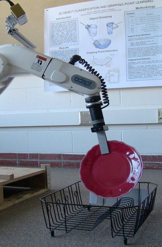
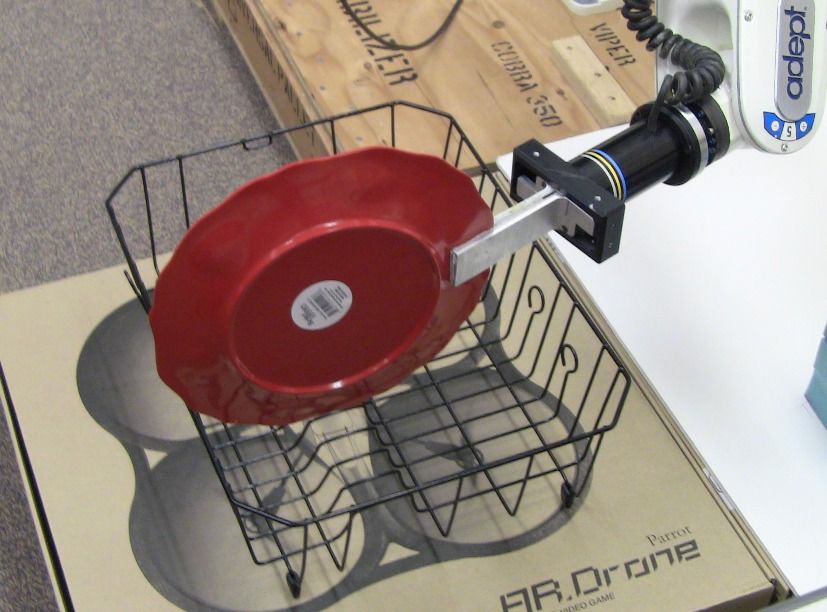
Fig. 2: Examples of a few objects (plate, martini glass, bowl) and placing areas (rack-1, rack-3, stemware holder). Full list is shown in
Table II.

  •   While some there is some prior work in finding ‘flat’           learning algorithms for grasping. Rao et al. [16] used point
      surfaces [3], we believe that our work is the first one         cloud to facilitate segmentation as well as learning grasps.
      that considers placing new objects in complex placing           Li et al. [17] combined object detection and grasping for
      areas.                                                          higher accuracy in grasping point detection. In some grasping
  •   Our learning algorithm captures features that indicate          works that assume known full 3D models (such as GraspIt
      stability of the placement as well as the ‘preferred’           [18]), different 3D locations/orientations of the hand are
      placing configuration for an object.                            evaluated for their grasp scores. Berenson et al. [19] consider
                                                                      grasping planning in complex scenes. Goldfeder [20] recently
                                                                      discussed a data-driven grasping approach. In this paper,
                     II. R ELATED W ORK                               we consider learning placements of objects in cluttered
   There is little previous work in placing objects, and it           placing areas—which is a different problem because our
is restricted to placing objects upright on ‘flat’ surfaces.          learning algorithm has to consider the object as well as the
Edsinger and Kemp [4] considered placing objects on a flat            environment to evaluate good placements. To the best of our
shelf. The robot first detected the edge of the shelf, and then       knowledge, we have not seen any work about learning to
explored the area with its arm to confirm the location of             place in complex situations.
the shelf. It used passive compliance and force control to                              III. S YSTEM OVERVIEW
gently and stably place the object on the shelf. This work               We frame the manipulation task of placing as a supervised
indicates that even for flat surfaces, unless the robot knows         learning problem. Given the features computed from the
the placing strategy very precisely, it takes good tactile sens-      point-clouds of the object and the environment, the goal of
ing and adjustment to implement placing without knocking              the learning algorithm is to find a good placing hypothesis.
the object down. Schuster et al. [3] recently developed a             As outlined in Fig. 3, the core part of our system is the
learning algorithm to detect clutter-free ‘flat’ areas where          placement classifier with supervised learning (yellow box in
an object can be placed. While these works assumes that               Fig. 3), which we will describe in detail in section IV-B. In
the given object is already in its upright orientation, some          this section, we briefly describe the other parts.
other related works consider how to find the upright or the              Our input to the system is the point-cloud of the object and
current orientation of the objects, e.g. Fu et al. [5] proposed       the placing area obtained from a Microsoft Kinect sensor.2
several geometric features to learn the upright orientation
from an object’s 3D model and Saxena et al. [6] predicted             A. Sampling of potential placements
the orientation of an object given its image. Our work is                Given the point-cloud of both the object and placing
different and complementary to these studies: we generalize           area, we first randomly sample several locations (100 in
placing environments from flat surfaces to more complex               our experiments) in the bounding box of the placing area
ones, and desired configurations are extended from upright            as the placement candidates. For each location, we have 18
to all other possible orientations that can make the best use         orientations (45 degrees rotation along each dimension) of
of the placing area.                                                  the object. For each of the 1800 candidate, we compute some
   Planning and rule-based approaches have been used in               features that capture stability and semantic preference (see
the past to move objects around. For example, Lozano-                 Section IV-A) and then use a learning algorithm to estimate
Perez et al. [7] considered picking up and placing objects            the score of it being a good placement.
by decoupling the planning problem into parts, and tested             B. Physics-based Simulation
on grasping objects and placing them on a table. Sugie et                In this work, we use rigid-body simulation to generate
al. [8] used rule-based planning in order to push objects on          training data for our supervised learning algorithm (see Fig. 5
a table surface. However, these approaches assume known               for some simulated placing tasks).
full 3D model of the objects, consider only flat surfaces, and
                                                                        2 Our learning algorithm presented in this paper is designed to work both
do not model preferred placements.
                                                                      with raw point-cloud obtained from a sensor (which is often noisy and
   In a related manipulation task, grasping, learning algo-           incomplete) as well as full 3D models. When 3D models of the object are
rithms have been shown to be promising. Saxena et al. [9],            available, we can optionally register the raw point-cloud to the database of
[10], [11], [12] used supervised learning with images and             the 3D models, using the Iterative Closest Point (ICP) algorithm [21], [22].
                                                                      The best matching object from the database is then used to represent the
partial point clouds as inputs to infer good grasps. Later,           completed geometry of the scanned object. We test both approaches in our
Le et al. [13] and Jiang et al. [14], [15] proposed new               experiments in Section V-F.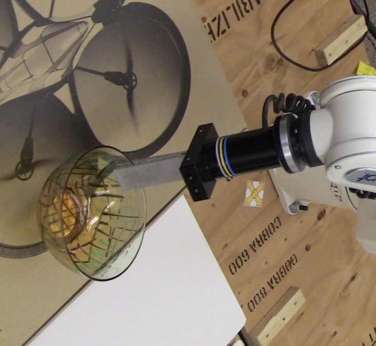
•   Preferred placements. Placements should also follow
                                                                                       common practice. For example, the plates should be
                                                                                       inserted into a dish-rack vertically and glasses should
                                                                                       be placed upside down on a stemware holder.
                                                                                   We group the features into three categories. In the follow-
                                                                                ing description, we use O0 to denote the point-cloud of the
Fig. 3: System Overview: The core part is the placement classifier              object O after being placed, and use B to denote the point-
(yellow box) which is trained using supervised learning to identify a           cloud of a placing area B. Let po be the 3D coordinate of
few candidates of placement configurations based on the perceived               a point o ∈ O0 from the object, and xt be the coordinate of
geometries of environments and objects. When we have access to
3D models, we perform 3D reconstruction on the raw point-cloud                  a point t ∈ B from the placing area.
before classification and we validate predicted placements via a                Supporting Contacts: Intuitively, an object is placed stably
rigid-body simulation before realization. However, these two steps              when it is supported by a wide spread of contacts. Hence,
are not compulsory, as demonstrated in our robotic experiments.                 we compute features that reflect the distribution of the
                                                                                supporting contacts. In particular, we choose the top 5%
   A placement defines the location T0 and orientation R0 of
                                                                                points in the placing area closest to the object (measured
the object in the environment. Its motion is computed by the
                                                                                by the vertical distance, ci shown in Fig. 4a) at the placing
rigid-body simulation at discrete time steps. At each time
                                                                                point. Suppose the k points are x1 , . . . , xk . We quantify the
step, we compute the kinetic energy change of the object
                                                                                set of these points by 8 features:
∆E = En − En−1 . The simulation runs until the kinetic
energy is almost constant (∆E < δ), in which a stable state                        1) Falling distance mini=1...k ci .
of the object can be assumed. Let Ts and Rs denote the                             2) Variance
                                                                                         Pk       in XY-plane and Z-axis respectively,
                                                                                                 0
stable state. We label the given placement as a valid one if                          k
                                                                                       1
                                                                                           i=1 (xi − x̄0 )2 , where x0i is the projection of xi
                                                                                                   Pk
the final state is close enough to the initial state, i.e. kTs −                      and x̄ = k i=1 x0i .
                                                                                            0    1

T0 k22 + kRs − R0 k22 < δs .                                                       3) Eigenvalues and ratios. We compute the three Eigen-
   Since the simulation itself has no knowledge of placing                            values (λ1 ≥ λ2 ≥ λ3 ) of the covariance matrix of
preferences, when creating the ground-truth training data, we                         these k points. Then we use them along with the ratios
manually labeled all the stable (as verified by the simulation)                       λ2 /λ1 and λ3 /λ2 as the features.
but un-preferred placements as negative examples.                                  Another common physics-based criterion is the center of
   We can also use the physics-based simulation to verify the                   mass (COM) of the placed object should be inside of (or
predicted placements when 3D models are available (see the                      close to) the region enclosed by contacts. So we calculate
second robotic experiment in Section V-F). This simulation                      the distance from the centroid of O0 to the nearest boundary
is computationally expensive,3 but we only need to do it for                    of the 2D convex hull formed by contacts projected to XY-
a few top placements.                                                           plane, Hcon . We also compute the projected convex hull of
                                                                                the whole object, Hobj . The area ratio of these two polygons
C. Realization
                                                                                SHcon /SHobj is included as another feature.
   To realize a placement decision, our robotic arm grasps                         Two more features representing the percentage of the
the object, moves it to the placing location with desired                       object points below or above the placing area are used to
orientation, and releases it. Our main goal in this paper is to                 capture the relative location.
learn how to place objects well, therefore in our experiments                   Caging: There are some placements where the object would
the kinematically feasible grasping points are pre-calculated.                  not be strictly immovable but is well confined within the
However, the motion plan that realizes the object being                         placing area. A pen being placed upright in a pen-holder
placed in the predicted location and orientation is computed                    is one example. While this kind of placement has only
using an inverse kinematics solver with a simple path planner                   a few supports from the pen-holder and may move under
[23]. The robot executes that plan and opens the gripper in                     perturbations, it is still considered a good one. We call this
order to release the object for placing.                                        effect ‘gravity caging.’4
                                                                                   We capture this by partitioning the point-cloud of the
                 IV. L EARNING A PPROACH
                                                                                environment and computing a battery of features for each
A. Features                                                                     zone. In detail, we divide the space around the object into
   In this section, we describe the features used in our                        3 × 3 × 3 zones. The whole divided space is the axis-aligned
learning algorithm. We design the features to capture the                       bounding box of the object scaled by 1.6, and the dimensions
following two properties:                                                       of the center zone are 1.05 times those of the bounding
   • Supports and Stability. The object should be able to                       box (Fig. 4b and 4c). The point-cloud of the placing area
     stay still after placing, and even better to be able to                    is partitioned into these zones labelled by Ψijk , i, j, k ∈
     stand small perturbations.                                                 {1, 2, 3}, where i indexes the vertical direction e1 , and j

  3 A single stability test takes 3.8 second on a 2.93GHz dual-core processor     4 This idea is motivated by previous works on force closure [24], [25] and
on average.                                                                     caging grasps [26].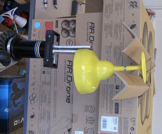
(a) supporting contacts         (b) caging (top view)     (c) caging (side view)      (d) histogram (top view)     (e) histogram (side view)
         Fig. 4: Illustration of features that are designed to capture the stability and preferred orientations in a good placement.

and k index the other two orthogonal directions, e2 and e3 ,                  We also compute the ratio of the two histograms as another
on horizontal plane.                                                       set of features, i.e., the number of points from O0 over
   From the top view, there are 9 regions (Fig. 4b), each of               the number of points from B in each cell. For numerical
which covers three zones in the vertical direction. The max-               stability, the maximum ratio is fixed to 10 in practice. For
imum height of points in each region is computed, leading                  our experiments, we set nz = 4 and nρ = 8 and hence have
to 9 features. We also compute the horizontal distance to the              96 histogram features.
object in three vertical levels from four directions (±e2 , ±e3 )             In total, we generate 145 features: 12 features for support-
(Fig. 4c). In particular, for each i = 1, 2, 3, we compute                 ing contacts, 37 features for caging, and 96 for the histogram
                                                                           features. They are used in the learning algorithm described
            di1 =             min           eT2 (po − xt )                 in the following sections.
                    xt ∈Ψi11 ∪Ψi12 ∪Ψi13
                           po ∈O0
                                                                           B. Max-Margin Learning
            di2 =             min           −eT2 (po − xt )                   Under the setting of a supervised learning problem, we are
                    xt ∈Ψi31 ∪Ψi32 ∪Ψi33
                           po ∈O0                                          given a dataset of labeled good and bad placements (see Sec-
                                                                   (1)
            di3 =             min           eT3 (po − xt )                 tion V-E), represented by their features. Our goal is to learn a
                    xt ∈Ψi11 ∪Ψi21 ∪Ψi31
                           po ∈O0                                          function of features that can determine whether a placement
            di4 =             min           −eT3 (po − xt )                is good or not. As support vector machines (SVMs) [2] have
                    xt ∈Ψi13 ∪Ψi23 ∪Ψi33                                   strong theoretical guarantees in the performance and have
                           po ∈O0
                                                                           been applied to many classification problems, we build our
and produce 12 additional features.                                        learning algorithm based on SVM.
   The degree of gravity-caging also depends on the relative                  Let φi ∈ Rp be the features of ith instance in the dataset,
height of the object and the caging placing area. Therefore,               and let yi ∈ {−1, 1} represent the label, where 1 is a good
we compute the histogram of the height of the points                       placement and −1 is not. For n examples in the dataset, the
surrounding the object. In detail, we first define a cylinder              soft-margin SVM learning problem [27] is formulated as:
centered at the lowest contact point with a radius that can                                          n
                                                                                   1   2
                                                                                             X
just cover O0 . Then points of B in this cylinder are divided                   min kθk2 + C     ξi
                                                                                   2
into nr × nθ parts based on 2D polar coordinates. Here, nr                                   i=1

is the number of radial divisions and nθ is the number of                        s.t. yi (θT φi − b) ≥ 1 − ξi ,      ξi ≥ 0, ∀1 ≤ i ≤ n            (2)
divisions in azimuth. The vector of the maximum height in
                                                                           where θ ∈ Rp are the parameters of the model, and ξ are the
each cell (normalized by the height of the object), H =
                                                                           slack variables. This method finds a separating hyperplane
(h1,1 , . . . , h1,nθ , . . . , hnr ,nθ ), is used as additional caging
                                                                           that maximizes the margin between the positive and the
features. To make H rotation-invariant, the cylinder is always
                                                                           negative examples.
rotated to align polar axis with the highest point, so that the
maximum value in H is always one of hi,1 , i = 1...nr . We                 C. Shared-sparsity Max-margin Learning
set nr = 4 and nθ = 4 for our experiments.                                    If we look at the objects and their placements in the
Histogram Features: Generally, a placement depends on the                  environment, we notice that there is an intrinsic difference
geometric shapes of both the object and the placing area.                  between different placing settings. For example, it seems
We compute a representation of the geometry as follows.                    unrealistic to assume placing dishes into a rack and hanging
We partition the point-cloud of O0 and of B radially and in                martini glasses upside down on a stemware holder share
Z-axis, centered at the centroid of O0 . Suppose the height of             exactly the same hypothesis, although they might agree on
the object is hO and its radius is ρmax . The 2D histogram                 a subset of attributes. While some attributes may be shared
with nz × nρ number of bins covers the cylinder with the                   across different objects and placing areas, there are some
radius of ρmax · nρ /(nρ − 2) and the height of hO · nz /(nz −             attributes that are specific to the particular setting. In such a
2), illustrated in Fig. 4d and 4e. In this way, the histogram              scenario, it is not sufficient to have either one single model
(number of points in each cell) can capture the global shape               or several completely independent models for each placing
of the object as well as the local shape of the environment                setting that tend to suffer from over-fitting. Therefore, we
around the placing point.                                                  propose to use a shared sparsity structure in our learning.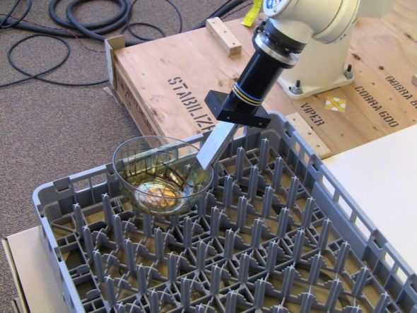
Fig. 5: Some snapshots from our rigid-body simulator showing different objects placed in different placing areas. Placing areas from left:
rack1, rack2, rack3, flat surface, pen holder, stemware holder, hook, hook and pen holder. Objects from left: mug, martini glass, plate,
bowl, spoon, martini glass, candy cane, disc and tuning fork. Rigid-body simulation is only used in labeling the training data and in half
of the robotic experiments when 3D object models are used (Section V-F).

   Say, we have M objects and N placing areas, thus making            learned models in the training data as the predicted score
a total of r = M N placing ‘tasks’ of particular object-area          (see Section V-B for different training settings).
pairs. Each task can have its own model but intuitively these
should share some parameters underneath. To quantify this                                  V. E XPERIMENTS
constraint, we use ideas from recent works [28], [29] that            A. Robot Hardware and Setup
attempt to capture the structure in the parameters of the                We use our PANDA (PersonAl Non-Deterministic Arm)
models. [28] used a shared sparsity structure for multiple            robot for our experiments, which comprises a Adept Viper
linear regressions. We apply their model to the classic soft-         s850 arm with six degrees of freedom, equipped with a
margin SVM.                                                           parallel plate gripper that can open to up to a maximum
   In detail, for r tasks, let Φi ∈ Rp×ni and Yi denote
                                                                      width of 5cm. The arm has a reach of 105cm, together with
training data and its corresponding label, where p is the size
                                                                      our gripper. The arm plus gripper has a repeatability of about
of the feature vector and ni is the number of data points
                                                                      1mm in XYZ positioning, but there is no force or tactile
in task i. We associate every task with a weight vector θi .
                                                                      feedback in this arm. We use a Microsoft Kinect sensor,
We decompose θi in two parts θi = Si + Bi : the self-
                                                                      mounted on the arm, for perceiving the point-clouds.
owned features Si and the shared features Bi . All self-owned
features, Si , should have only a few non-zero values so              B. Learning Scenarios
that they can reflect individual differences to some extent
                                                                         In real-world placing, the robot may or may not have seen
but would not become dominant in the final model. Shared
                                                                      the placing locations (and the objects) before. Therefore, we
features, Bi , need not have identical values, but should share
                                                                      train our algorithm for four different scenarios:
similar sparsity structure across tasks. In other words, for
each feature, they                                                       1)   Same Environment Same Object (SESO),
                 P should  j
                               all either be active
                                                  Ppor non-active.
                                                               j
Let kSk1,1 =            |S   |      kBk                                  2)   Same Environment New Object (SENO),
                    i,j   i    and         1,∞ =    j=1 maxi |Bi |.
Our new goal function is now:                                            3)   New Environment Same Object (NESO),
                     Pr  1              2     Pni                      4)   New Environment New Object (NENO).
        min              i=1 2    kθ i k 2 + C   j=1 ξi,j   +
   θi ,bi ,i=1,...,r                                                     If the object (environment) is ‘same’, then only this object
                             λS kSk1,1 + λB kBk1,∞                    (environment) is included in the training data. If it is ’new’,
     subject to Yij (θiT Φji + bi ) ≥ 1 − ξi,j , ξi,j ≥ 0             then all other objects (environments) are included except the
                            ∀1 ≤ i ≤ r, 1 ≤ j ≤ ni                    one for test. Through these four scenarios, we would be able
                      θi = Si + Bi , ∀1 ≤ i ≤ r                (3)    to observe the algorithm’s performance thoroughly.
When testing in a new scenario, different models vote to
                                                                      C. Baseline Methods
determine the best placement.
   While this modification results in superior performance               We compare our algorithm with the following three heuris-
with new objects in new placing areas, it requires one model          tic methods:
per object-area pair and therefore it would not scale to a            Chance. The location and orientation is randomly sampled
large number of objects and placing areas.                            within the bounding box of the area and guaranteed to be
   We transform this optimization problem into a standard             ‘collision-free.’
quadratic programming (QP) problem by introducing auxil-              Flat-surface-upright rule. Several methods exist for detect-
iary variables to substitute for the absolute and the maximum         ing ‘flat’ surfaces [3], and we consider a placing method
value terms. Unlike Eq. (2) which decomposes into r sub-              based on finding flat surfaces. In this method, objects would
problems, the optimization problem in Eq. (3) becomes                 be placed with pre-defined upright orientation on the surface.
larger, and hence takes a lot of computational time to                When no flat surface can be found, a random placement
learn the parameters. However, inference is still fast since          would be picked. Note that this heuristic actually uses more
predicting the score is simply the dot product of the features        information than our method.
with the learned parameters. During the test, if the task is          Finding lowest placing point. For many placing areas,
in the training set, then its corresponding model is used to          such as dish-racks or containers, a lower placing point often
compute the scores. Otherwise we use a voting system, in              gives more stability. Therefore, this heuristic rule chooses
which we use the average of the scores evaluated by each              the placing point with the lowest height.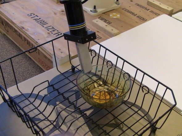
TABLE I: Average performance of our algorithm using different         We get close to perfect results for SESO case—i.e., the
features on the SESO scenario.                                     learning algorithm can very reliably predict object place-
               chance   contact   caging   histogram    all        ments if a known object was being placed in a previously
        R0      29.4      1.4       1.9        1.3     1.0
        P@5     0.10     0.87      0.77       0.86     0.95        seen location. The performance is still very high for SENO
        AUC     0.54     0.89      0.83       0.86     0.95        and NESO (i.e., when the robot has not seen the object or
                                                                   the environment before), where the first correct prediction is
D. Evaluation Metrics                                              ranked 2.3 and 2.5 on average. This means we only need
                                                                   to perform simulation for about three times. There are some
  We evaluate our algorithm’s performance on the following         challenging tasks in the NESO case, such as placing on the
metrics:                                                           hook and in the pen-holder when the algorithm has never
  •   R0 : Rank of the first valid placement. (R0 = 1 ideally.)    seen these placing areas before. In those cases, the algorithm
  •   P@5: In top 5 candidates, the fraction of valid place-       is biased by the training placing area and thus tends to predict
      ments.                                                       horizontal placements.
  •   AUC: Area under ROC Curve [30], a classification                The last learning scenario NENO is extremely
      metric computed from all the candidates.                     challenging—for each task (of an object-area pair),
  •   Ps : Success-rate (in %) of placing the object stably with   the algorithm is trained without either the object or the
      the robotic arm.                                             placing area in the training set. In this case, R0 increases
  •   Pp : Success-rate (in %) of placing the object stably in     to 8.9 with joint SVM, and to 5.4 using independent SVM
      preferred configuration with the robotic arm.                with voting. However, shared sparsity SVM (the last row
                                                                   in the table) helps to reduce the average R0 down to 2.1.
                                                                   While shared sparsity SVM outperforms other algorithms,
E. Learning Experiments
                                                                   the result also indicates that independent SVM with voting
   For evaluating our learning algorithm, we considered 7          is better than joint SVM. This could be due to the large
placing areas (3 racks, a flat surface, pen holder, stemware       variety in the placing situations in the training set. Thus
holder and hook) and 8 objects (mug, martini glass, plate,         imposing one model for all tasks decreases the performance.
bowl, spoon, candy cane, disc and tuning fork), as shown in        We also observed that in cases where the placing strategy is
Fig. 5. We generated one training and one test dataset for         very different from the ones trained on, the shared sparsity
each object-environment pair. Each training/test dataset con-      SVM does not perform well. For example, R0 is 7.0 for
tains 1800 random placements with different locations and          spoon-in-pen-holder and is 5.0 for disk-on-hook. This could
orientations. After eliminating placements with collisions, we     potentially be addressed by expanding the training dataset.
have 37655 placements in total. These placements were then
labeled by rigid-body simulation (see Section III-B).              F. Robotic Experiments
   Table I shows the average performance when we use                  We conducted experiments on our PANDA robot, using
different types of features: supporting contacts, caging and       the same dataset for training. We tested 10 different placing
geometric signatures. While all the three types of features        tasks with 10 trials for each. A placement was considered
outperform chance, combining them together gives the high-         successful if it was stable (i.e., the object remained still for
est performance under all evaluation metrics.                      more than a minute) and in its preferred orientation (within
   Next, Table II shows the comparison of three heuristic          ±15◦ of the ground-truth orientation after placing).
methods and three variations of SVM learning algorithms: 1)           Table III shows the results for three objects being placed
joint SVM, where one single model is learned from all the          by the robotic arm in four placing scenarios (see the bottom
placing tasks in the training dataset; 2) independent SVM,         six rows). We obtain a 94% success rate in placing the
which treats each task as a independent learning problem           objects stably in SESO case, and 92% if we disqualify
and learns a separate model per task; 3) shared sparsity           those stable placements that were not preferred ones. In the
SVM (Section IV-B), which also learns one model per task           NENO case, we achieve 82% performance for stable placing,
but with parameter sharing. Both independent and shared            and 72% performance for preferred placing. Figure 6 shows
sparsity SVM use voting to rank placements for the test case.      several screenshots of our robot placing the objects. There
   Table II shows that all the learning methods (last six          were some cases where the martini glass and the bowl were
rows) outperform heuristic rules under all evaluation metrics.     placed horizontally in rack1. In these cases, even though the
Not surprisingly, the chance method performs poorly (with          placements were stable, they were not counted as preferred.
Prec@5=0.1 and AUC=0.49) because there are very few                Even small displacement errors while inserting the martini
preferred placements in the large sampling space of possible       glass in the narrow slot of the stemware holder often resulted
placements. The two heuristic methods perform well in some         in a failure. In general, several failures for the bowl and the
obvious cases such as using flat-surface-upright method for        martini glass were due to incomplete capture of the point-
table or lowest-point method for rack1. However, their per-        cloud which resulted in the object hitting the placing area
formance varies significantly in non-trivial cases, including      (e.g., the spikes in the dish-rack).
the stemware holder and the hook. This demonstrates that it           In order to analyze the errors caused by the incomplete
is hard to script a placing rule that works universally.           point-clouds, we did another experiment in which we use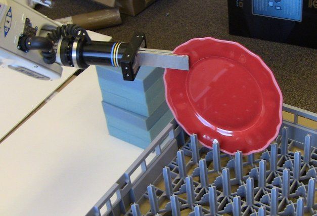
TABLE II: Learning experiment statistics: The performance of different learning algorithms in different scenarios is shown. The top
three rows are the results for baselines, where no training data is used. The fourth to sixth row is trained and tested for the SESO, SENO
and NESO case respectively using independent SVMs. The last three rows are trained using joint, independent and shared sparsity SVMs
respectively for the NENO case.
Listed object-wise, averaged over the placing areas.
plate mug martini bowl candy cane disc spoon tuning fork
flat, flat, flat, 3 racks, flat, flat, hook, flat, hook, flat, flat, Average
3 racks 3 racks stemware holder 3 racks pen holder pen holder pen holder pen holder
R0 P@5 AUC R0 P@5 AUC R0 P@5 AUC R0 P@5 AUC R0 P@5 AUC R0 P@5 AUC R0 P@5 AUC R0 P@5 AUC R0 P@5 AUC
NENO indep. baseline
chance 4.0 0.20 0.49 5.3 0.10 0.49 6.8 0.12 0.49 6.5 0.15 0.50 102.7 0.00 0.46 32.7 0.00 0.46 101.0 0.20 0.52 44.0 0.00 0.53 29.4 0.10 0.49
flat-up 4.3 0.45 0.38 11.8 0.50 0.78 16.0 0.32 0.69 6.0 0.40 0.79 44.0 0.33 0.51 20.0 0.40 0.81 35.0 0.50 0.30 35.5 0.40 0.66 18.6 0.41 0.63
lowest 27.5 0.25 0.73 3.8 0.35 0.80 39.0 0.32 0.83 7.0 0.30 0.76 51.7 0.33 0.83 122.7 0.00 0.86 2.5 0.50 0.83 5.0 0.50 0.76 32.8 0.30 0.80
SESO 1.3 0.90 0.90 1.0 0.85 0.92 1.0 1.00 0.95 1.0 1.00 0.92 1.0 0.93 1.00 1.0 0.93 0.97 1.0 1.00 1.00 1.0 1.00 1.00 1.0 0.95 0.95
SENO 1.8 0.65 0.75 2.0 0.50 0.76 1.0 0.80 0.83 4.3 0.45 0.80 1.7 0.87 0.97 4.3 0.53 0.78 1.0 1.00 0.98 1.5 0.60 0.96 2.3 0.65 0.83
NESO 1.0 0.85 0.76 1.5 0.70 0.85 1.2 0.88 0.86 1.5 0.80 0.84 2.7 0.47 0.89 3.7 0.47 0.85 5.5 0.10 0.72 8.0 0.00 0.49 2.5 0.62 0.81
joint 8.3 0.50 0.78 2.5 0.65 0.88 5.2 0.48 0.81 2.8 0.55 0.87 16.7 0.33 0.76 20.0 0.33 0.81 23.0 0.20 0.66 2.0 0.50 0.85 8.9 0.47 0.81
indep. 2.0 0.70 0.86 1.3 0.80 0.89 1.2 0.86 0.91 3.0 0.55 0.82 9.3 0.60 0.87 11.7 0.53 0.88 23.5 0.40 0.82 2.5 0.40 0.71 5.4 0.64 0.86
shared 1.8 0.70 0.84 1.8 0.80 0.85 1.6 0.76 0.90 2.0 0.75 0.91 2.7 0.67 0.88 1.3 0.73 0.97 7.0 0.40 0.92 1.0 0.40 0.84 2.1 0.69 0.89
Listed placing area-wise, averaged over the objects.
rack1 rack2 rack3 flat pen holder hook stemware holder
plate, mug, plate, mug, plate, mug, all candy cane, disc, candy cane, martini Average
martini, bowl martini, bowl martini, bowl objects spoon, tuningfork disc
R0 P@5 AUC R0 P@5 AUC R0 P@5 AUC R0 P@5 AUC R0 P@5 AUC R0 P@5 AUC R0 P@5 AUC R0 P@5 AUC
NENO indep. baseline
chance 3.8 0.15 0.53 5.0 0.25 0.49 4.8 0.15 0.48 6.6 0.08 0.48 128.0 0.00 0.50 78.0 0.00 0.46 18.0 0.00 0.42 29.4 0.10 0.49
flat-up 2.8 0.50 0.67 18.3 0.05 0.47 4.8 0.20 0.60 1.0 0.98 0.91 61.3 0.05 0.45 42.0 0.00 0.45 65.0 0.00 0.58 18.6 0.41 0.63
lowest 1.3 0.75 0.87 22.0 0.10 0.70 22.0 0.15 0.80 4.3 0.23 0.90 60.3 0.60 0.85 136.5 0.00 0.71 157.0 0.00 0.56 32.8 0.30 0.80
SESO 1.0 1.00 0.91 1.3 0.75 0.83 1.0 1.00 0.93 1.0 0.95 1.00 1.0 1.00 0.98 1.0 1.00 1.00 1.0 1.00 1.00 1.0 0.95 0.95
SENO 1.25 0.70 0.83 2.5 0.40 0.66 3.5 0.45 0.72 1.4 0.93 0.96 3.5 0.55 0.89 2.5 0.60 0.81 - - - 2.3 0.65 0.83
NESO 1 1.00 0.83 1.5 0.60 0.77 1.3 0.75 0.82 2.9 0.65 0.86 4.0 0.20 0.70 6.5 0.20 0.81 1.0 1.00 0.79 2.5 0.62 0.81
joint 1.8 0.60 0.92 2.5 0.70 0.84 8.8 0.35 0.70 2.4 0.63 0.86 20.5 0.25 0.76 34.5 0.00 0.69 18.0 0.00 0.75 8.9 0.47 0.81
indep. 1.3 0.70 0.85 2.0 0.55 0.88 2.5 0.70 0.86 1.9 0.75 0.89 12.3 0.60 0.79 29.0 0.00 0.79 1.0 1.00 0.94 5.4 0.64 0.86
shared 1.8 0.75 0.88 2.0 0.70 0.86 2.3 0.70 0.84 1.3 0.75 0.92 4.0 0.60 0.88 3.5 0.40 0.92 1.0 0.80 0.95 2.1 0.69 0.89
TABLE III: Robotic experiments. The algorithm is trained using shared sparsity SVM under the two learning scenarios: SESO and
NENO. 10 trials each are performed for each object-placing area pair. In the experiments with object models, R0 stands for the rank of
first predicted placements passed the stability test. In the experiments without object models, we do not perform stability test and thus R0
is not applicable. In summary, robotic experiments show a success rate of 98% when the object has been seen before and its 3D model
is available, and show a success-rate of 82% (72% when also considering semantically correct orientations) when the object has not been
seen by the robot before in any form.
plate martini bowl
Average
rack1 rack3 flat rack1 rack3 flat stem. rack1 rack3 flat
R0 1.0 1.0 1.0 1.0 1.0 1.0 1.0 1.0 1.0 1.0 1.0
w/o obj models w/ obj models
SESO Ps (%) 100 100 100 100 100 100 80 100 100 100 98
Pp (%) 100 100 100 100 100 100 80 100 100 100 98
R0 1.8 2.2 1.0 2.4 1.4 1.0 1.2 3.4 3.0 1.8 1.9
NENO Ps (%) 100 100 100 80 100 80 100 100 100 100 96
Pp (%) 100 100 100 60 100 80 100 80 100 100 92
R0 - - - - - - - - - - -
SESO Ps (%) 100 80 100 80 100 100 80 100 100 100 94
Pp (%) 100 80 100 80 80 100 80 100 100 100 92
R0 - - - - - - - - - - -
NENO Ps (%) 80 60 100 80 80 100 70 70 100 80 82
Pp (%) 80 60 100 60 70 80 60 50 80 80 72
3D models to reconstruct the full geometry. Furthermore, objects. Some of the cases are quite tricky, for example
since we had access to a full solid 3D model, we verified placing the martini-glass hanging from the stemware holder.
the stability of the placement using the rigid-body simulation Videos of our robot placing these objects is available at:
(Section III-B) before executing it on the robot. If it failed http://pr.cs.cornell.edu/placingobjects
the stability test, we would try the placement with the next
highest score until it would pass the test. VI. C ONCLUSION AND D ISCUSSION
In this setting with a known library of object models, we In this paper, we considered the problem of placing objects
obtain a 98% success rate in placing the objects in SESO in various types of placing areas, especially when the objects
case. The robot failed only in one experiment, when the mar- and the placing areas may not have been seen by the robot
tini glass could not fit into the narrow stemware holder due before. We first presented features that contain information
to a small displacement occurred in grasping. In the NENO about stability and preferred orientations. We then used a
case, we achieve 96% performance in stable placements and shared-sparsity SVM learning approach for predicting the
92% performance in preferred placements. This experiment top placements. In our extensive learning and robotic ex-
indicates that with better sensing of the point-clouds, our periments, we showed that different objects can be placed
learning algorithm can give better performance. successfully in several environments, including flat surfaces,
Fig. 6 shows several screenshots of our robot placing several dish-racks, a stemware holder and a hook.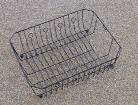
Fig. 6: Some screenshots of our robot placing different objects in several placing areas. In the examples above, the robot placed the objects
in stable as well as preferred configuration, except for the top right image where a bowl is placed stably in upright orientation on rack-1.
A more preferred orientation is upside down.

   There still remain several issues for placing objects that                 [13] Q. Le, D. Kamm, A. Kara, and A. Ng, “Learning to grasp objects
we have not addressed yet, such as using force or tactile                          with multiple contact points,” in ICRA. IEEE, 2010, pp. 5062–5069.
                                                                              [14] Y. Jiang, S. Moseson, and A. Saxena, “Efficient Grasping from RGBD
feedback while placing. We also need to consider detecting                         Images: Learning using a new Rectangle Representation,” ICRA, 2011.
the appropriate placing areas in an environment for an object                 [15] Y. Jiang, J. Amend, H. Lipson, and A. Saxena, “Learning hardware
(e.g., table vs ground for a placing a shoe), and how to place                     agnostic grasps for a universal jamming gripper,” in ICRA, 2012.
                                                                              [16] D. Rao, Q. Le, T. Phoka, M. Quigley, A. Sudsang, and A. Ng,
multiple objects in the tasks of interest such as arranging a                      “Grasping Novel Objects with Depth Segmentation,” in IROS, 2010.
disorganized kitchen or cleaning a cluttered room.                            [17] C. Li, A. Kowdle, A. Saxena, and T. Chen, “Towards holistic scene
                                                                                   understanding: Feedback enabled cascaded classification models,” in
                            R EFERENCES                                            NIPS, 2010.

 [1] Y. Jiang, C. Zheng, M. Lim, and A. Saxena, “Learning to place            [18] M. T. Ciocarlie and P. K. Allen, “On-line interactive dexterous
     new objects,” in Workshop on Mobile Manipulation: Learning to                 grasping,” in Eurohaptics, 2008.
     Manipulate, 2011.                                                        [19] D. Berenson, R. Diankov, K. Nishiwaki, S. Kagami, and J. Kuffner,
 [2] C. Cortes and V. Vapnik, “Support-vector networks,” Machine learn-            “Grasp planning in complex scenes,” in Humanoid Robots, 2009.
     ing, 1995.                                                               [20] C. Goldfeder, M. Ciocarlie, J. Peretzman, H. Dang, and P. Allen,
 [3] M. Schuster, J. Okerman, H. Nguyen, J. Rehg, and C. Kemp, “Perceiv-           “Data-driven grasping with partial sensor data,” in IROS, 2009.
     ing clutter and surfaces for object placement in indoor environments,”   [21] S. Rusinkiewicz and M. Levoy, “Efficient variants of the icp algo-
     in Int’ Conf Humanoid Robots, 2010.                                           rithm,” in 3DIM, 2001.
 [4] A. Edsinger and C. Kemp, “Manipulation in human environments,” in        [22] N. Gelfand, N. J. Mitra, L. J. Guibas, and H. Pottmann, “Robust global
     Int’l Conf Humanoid Robots. IEEE, 2006.                                       registration,” in Eurographics Symp Geometry Processing, 2005.
 [5] H. Fu, D. Cohen-Or, G. Dror, and A. Sheffer, “Upright orientation of     [23] S. LaValle and J. Kuffner Jr, “Randomized kinodynamic planning,” in
     man-made objects,” ACM Trans. Graph., vol. 27, pp. 42:1–42:7, 2008.           Robotics and Automation, 1999. Proceedings. 1999 IEEE International
 [6] A. Saxena, J. Driemeyer, and A. Y. Ng, “Learning 3-d object orienta-          Conference on, vol. 1. IEEE, 1999, pp. 473–479.
     tion from images,” in ICRA, 2009.                                        [24] V. Nguyen, “Constructing stable force-closure grasps,” in ACM Fall
 [7] T. Lozano-Pérez, J. Jones, E. Mazer, and P. O’Donnell, “Task-level           joint computer conf, 1986.
     planning of pick-and-place robot motions,” Computer, 2002.               [25] J. Ponce, D. Stam, and B. Faverjon, “On computing two-finger force-
 [8] H. Sugie, Y. Inagaki, S. Ono, H. Aisu, and T. Unemi, “Placing objects         closure grasps of curved 2D objects,” IJRR, 1993.
     with multiple mobile robots-mutual help using intention inference,” in   [26] R. Diankov, S. Srinivasa, D. Ferguson, and J. Kuffner, “Manipulation
     ICRA, 1995.                                                                   planning with caging grasps,” in Humanoid Robots, 2008.
 [9] A. Saxena, J. Driemeyer, and A. Ng, “Robotic grasping of novel           [27] T. Joachims, Making large-Scale SVM Learning Practical. MIT-Press,
     objects using vision,” IJRR, 2008.                                            1999.
[10] A. Saxena, L. Wong, and A. Y. Ng, “Learning grasp strategies with        [28] A. Jalali, P. Ravikumar, S. Sanghavi, and C. Ruan, “A Dirty Model
     partial shape information,” in AAAI, 2008.                                    for Multi-task Learning,” NIPS, 2010.
[11] A. Saxena, J. Driemeyer, J. Kearns, and A. Ng, “Robotic grasping of      [29] C. Li, A. Saxena, and T. Chen, “θ-mrf: Capturing spatial and semantic
     novel objects,” in Neural Information Processing Systems, 2006.               structure in the parameters for scene understanding,” in NIPS, 2011.
[12] A. Saxena, “Monocular depth perception and robotic grasping of novel     [30] J. Hanley and B. McNeil, “The meaning and use of the area under a
     objects,” Ph.D. dissertation, Stanford University, 2009.                      receiver operating (roc) curvel characteristic,” Radiology, 1982.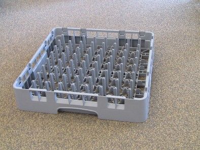
You can also read