Large-Scale Whale-Call Classification by Transfer Learning on Multi-Scale Waveforms and Time-Frequency Features - MDPI
←
→
Page content transcription
If your browser does not render page correctly, please read the page content below
applied
           sciences
Article
Large-Scale Whale-Call Classification by Transfer
Learning on Multi-Scale Waveforms and
Time-Frequency Features
Lilun Zhang 1,† , Dezhi Wang 1, *,† , Changchun Bao 1 , Yongxian Wang 1 and Kele Xu 2
 1   College of Meteorology and Oceanography, National University of Defense Technology,
     Changsha 410000, China; zll0434@163.com (L.Z.); baochangchun1979@163.com (C.B.);
     yxwang@nudt.edu.cn (Y.W.)
 2   College of Computer Science and Technology, National University of Defense Technology,
     Changsha 410000, China; kelele.xu@gmail.com
 *   Correspondence: wang_dezhi@hotmail.com; Tel.: +86-0731-8451-1412
 †   The first two authors have the equal contributions.

 Received: 27 January 2019; Accepted: 7 March 2019; Published: 12 March 2019

 Abstract: Whale vocal calls contain valuable information and abundant characteristics that are
 important for classification of whale sub-populations and related biological research. In this study,
 an effective data-driven approach based on pre-trained Convolutional Neural Networks (CNN)
 using multi-scale waveforms and time-frequency feature representations is developed in order to
 perform the classification of whale calls from a large open-source dataset recorded by sensors carried
 by whales. Specifically, the classification is carried out through a transfer learning approach by
 using pre-trained state-of-the-art CNN models in the field of computer vision. 1D raw waveforms
 and 2D log-mel features of the whale-call data are respectively used as the input of CNN models.
 For raw waveform input, windows are applied to capture multiple sketches of a whale-call clip at
 different time scales and stack the features from different sketches for classification. When using the
 log-mel features, the delta and delta-delta features are also calculated to produce a 3-channel feature
 representation for analysis. In the training, a 4-fold cross-validation technique is employed to reduce
 the overfitting effect, while the Mix-up technique is also applied to implement data augmentation
 in order to further improve the system performance. The results show that the proposed method
 can improve the accuracies by more than 20% in percentage for the classification into 16 whale pods
 compared with the baseline method using groups of 2D shape descriptors of spectrograms and the
 Fisher discriminant scores on the same dataset. Moreover, it is shown that classifications based on
 log-mel features have higher accuracies than those based directly on raw waveforms. The phylogeny
 graph is also produced to significantly illustrate the relationships among the whale sub-populations.

 Keywords: deep learning; transfer learning; convolutional neural network; whale-call classification

1. Introduction
     Acoustic methods are an established technique to monitor marine mammal populations and their
behaviors. The automated detection and classification of marine mammal vocalizations is a central
aim of these methods. Whales produce a series of whistles and other complex sounds to survey their
surroundings, hunt for food, and communicate with each other. The different types of whales are
gregarious living within socially stable family units known as ‘pods’, such as killer whales (Orcinus
orca) [1,2] and pilot whales (Globicephala spp.) [3]. Within a pod, whales share a unique repertoire
(also known as dialect) of stereotyped calls, which are comprised of a complex pattern of pulsed and
tonal elements [4]. Classification of killer whale and pilot whale calls is of great importance not only

Appl. Sci. 2019, 9, 1020; doi:10.3390/app9051020                               www.mdpi.com/journal/applsci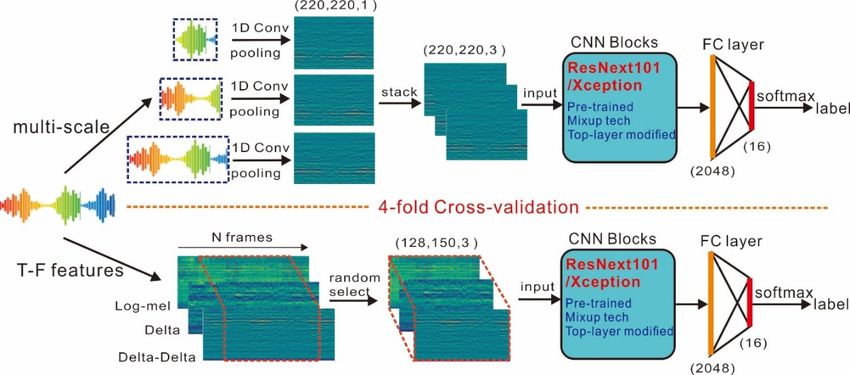
Appl. Sci. 2019, 9, 1020                                                                                2 of 11

for a better understanding of whale societies, but also for promoting investigative research on large
underwater acoustic datasets.
      With the continuous development of devices such as hydrophones deployed from ships, or digital
acoustic recording tags (DTAGs) placed on marine mammals, large datasets of whale sound samples
are increasingly being acquired. Often, an expert must analyze these large, volumetric datasets.
Such manual analysis is a very labor-intensive task that would greatly benefit from automation.
Different approaches for analyzing large audio datasets are being developed. Most methods are
feature-based classifiers, which generally first extract or search for deterministic features of audio data
in the time or frequency domain and then apply classification algorithms. Characterization methods
based on short-time overlapping segments with the short-time Fourier and the wavelet packet
transforms have been proposed to classify blue whale calls [5]. A large amount of the acoustic dataset
titled Directional Autonomous Seafloor Acoustic Recorders (DASARs) is used to test the performance
of contour tracing methods and image segmentation techniques in detecting and classifying bowhead
whale calls [6]. Recently in the classification of humpback whale social calls, some researchers apply
PCA-based and connected-component-based methods to derive features from relative power in the
frequency bins of spectrograms and a supervised Hidden Markov Model (HMM) algorithm is then
used as a classifier to investigate the classification feasibility [7]. A generalized automated detection
and classification system (DCS) was developed to efficiently and accurately identify low-frequency
baleen whale calls in order to tackle the large volume of acoustic data and reduce the laborious task [8].
In 2014, Lior Shamir etc. [9] proposed an automatic method for analyzing large acoustic datasets from
the Whale FM project [10] and studied the differences between sounds of different sub-populations
of whales. In their study, groups of 2D image-like features of whale calls were extracted by using
the Wndchrm toolbox [11] for biological image analysis and the Fisher discriminant scores algorithm,
which include FFT features, wavelet features, edge features, and so on. The significant features
were then used to classify or evaluate the similarity between the different populations of samples
without expert-based auditing. Although this work has already made progress in the unsupervised
classification and similarity analysis of large acoustic datasets of whale calls, it still highly relies on the
effectiveness of different polynomial decomposition techniques and the Fisher scores algorithm.
      Nowadays, as a class of highly non-linear machine learning models, Convolutional Neural
Networks (CNNs) are becoming very popular, having achieved state-of-the-art results in image
recognition [12] and other fields. In particular, the CNN network can combine hierarchical feature
extraction and classification together, which plays a role as an automated feature extractor and
classifier at the same time. In the field of acoustic signal processing, CNN-based models are also
adopted in speech recognition systems [13] for large-scale speech datasets, which shows a great
improvement in performance [14] as opposed to more traditional classifiers. More recently, some
research [15,16] has demonstrated that a basic CNN could generally outperform existing methods
for environmental sound classification, provided sufficient data. Moreover, the applicability of basic
CNN models is also being explored for the bio-acoustic task of whale call detection, such as with
respect to North Atlantic right whale calls [17] and Humpback whale calls [18]. The recent successful
applications of CNN-based models to time series classification have motivated studies aiming for
better input representations of audio signals in order to train the CNN networks more efficiently.
Various time-frequency representations, such as spectrograms, can typically offer a rich representation
of the temporal and spectral structure of the original audios. A comparative study between different
forms of commonly used time-frequency representations is conducted to evaluate their impact on
the CNN classification performance of audio data [19]. For superior feature representations for the
purposes of time series classification, a Multi-scale time-frequency analysis framework is also proposed
to automatically extract features at different scales and frequencies [20]. To thoroughly explore the
potential of CNNs on classification of optical remote sensing imagery data, a detailed investigation
of the performance of seven well-known CNN architectures is presented in [21,22], where both two
Appl. Sci. 2019, 9, 1020 3 of 11
Appl. Sci. 2019, 9, x FOR PEER REVIEW 3 of 12
types of training, i.e., fine-tuning of a pre-trained CNN and training of a CNN from scratch, were
respectively
This study applied
aimsto toobtain
apply results.
CNN to efficiently extract the informative features from large datasets
This calls
of whale studyfor aims to apply CNN
classification and to efficiently
similarity extract the
analysis. Threeinformative features from
main contributions large
of our datasets
work of
can be
whale
summarizedcalls for as: classification
(1) To overcome andthesimilarity
difficultyanalysis.
of lack ofThree main
sufficient contributions
training data andofmake our work
use of can
the
be summarized
excellent as: (1) To overcome
CNN architectures well trained theondifficulty
a large set of of
lack of sufficient
labeled training data
data in computer visionand makea
[23,24],
use
means of of
the excellent
transfer CNNwas
learning architectures
implemented well
bytrained
fine-tuningon athe large set CNN
trained of labeled
models, data
i.e.,inResNext101
computer
vision [23,24], a means of transfer learning was implemented by fine-tuning
and Xception [25], on whale-call data to perform the classification task. (2) Both the raw waveforms the trained CNN models,
i.e.,
fromResNext101
the multi-scale and sketches
Xceptionof[25], on whale-call
the whale call audiosdataandto perform
the log-melthetime-frequency
classification task. (2) Both the
representations
raw
werewaveforms
explored in from
orderthetomulti-scale
achieve ansketches of the representation
ideal feature whale call audios as and the log-mel
the input of CNN time-frequency
network. (3)
representations were explored
To ensure the convergence of in order
deep to achieve
neural networks,an ideal feature representation
a Mix-up-based as the input
data augmentation of CNN
technique
network.
[26] was also (3) Toemployed,
ensure thewhich convergence of deep neural
is advantageous networks, aincreasing
in significantly Mix-up-based data augmentation
the number of training
technique
data for fully [26]simulating
was also employed, which is advantageous
the CNN networks. (4) In addition, in the
significantly
similarityincreasing
analysis was the carried
numberout of
training data for fully simulating the CNN networks. (4) In addition,
based on the ‘likelihood’ output of the Softmax layer, while the whale phylogeny was drawn tothe similarity analysis was carried
out based
further on the ‘likelihood’
illustrate the detailed output of theamong
relationship Softmax layer, while
different whalethe whale phylogeny
sub-populations. The was drawn
code to
can be
further illustrate the detailed relationship among different
accessed in the Github (https://github.com/Blank-Wang/whale-call-classification). whale sub-populations. The code can be
accessed in the Github (https://github.com/Blank-Wang/whale-call-classification).
2. Methodology
2. Methodology
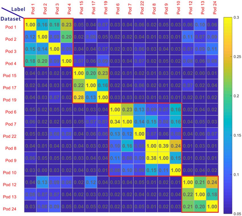
As illustrated in Figure 1, the proposed method consists of two main branches, respectively
usingAstwo illustrated
different in Figure
types of1, the proposed
inputs for CNNmethod consists
models of two main
to perform the branches, respectively
classification, i.e., 1Dusing
raw
two different types of inputs for CNN models to perform the classification,
waveforms and 2D time-frequency features. The CNN models are pre-trained by a large dataset of i.e., 1D raw waveforms
and 2D time-frequency
labeled image samples features. The CNN[12]
titled ‘ImageNet’ models
and are canpre-trained
be fine-tuned by aby large dataset
using of labeled
a whale-call image
training
samples
dataset through a 4-fold cross-validation. The performance of the system is finally evaluated4-fold
titled ‘ImageNet’ [12] and can be fine-tuned by using a whale-call training dataset through a on a
cross-validation. The
whale-call validation dataset.performance of the system is finally evaluated on a whale-call validation dataset.
Figure 1. Illustration of the proposed architecture.
2.1. Classification on
2.1. Classification on Raw
Raw Waveforms
Waveforms
Extracting featuresdirectly
Extracting features directlyfrom
fromrawrawwhale-call
whale-call time
time series
series by using
by using neural
neural networks
networks is an is an
end-
end-to-end
to-end wayway to doto the
do the classification,
classification, which
which avoids
avoids having
having totopre-process
pre-processthe theraw
rawaudio
audio signals
signals into
into
other forms of inputs such as spectrograms for classifiers. It is actually a natural
other forms of inputs such as spectrograms for classifiers. It is actually a natural way to apply theway to apply the deep
learning techniques
deep learning to do the
techniques classification
to do directlydirectly
the classification on raw on whale-call waveforms.
raw whale-call Due to the
waveforms. Due fact
tothat
the
different kinds of whale sounds may require feature representations at different
fact that different kinds of whale sounds may require feature representations at different time scales, time scales, we use
windows to randomly
we use windows capture the
to randomly sketches
capture the of raw audio
sketches time
of raw seriestime
audio at different
series attime scales.time
different As shown
scales.
in Figure 1, the proposed architecture consists of a set of parallel 1D convolutional
As shown in Figure 1, the proposed architecture consists of a set of parallel 1D convolutional layers with different
layers
filter sizes and strides to learn feature representations with multi-temporal resolutions.
with different filter sizes and strides to learn feature representations with multi-temporal resolutions. In this setup,
high-frequency features can be learned by convolutional filters with a short size
In this setup, high-frequency features can be learned by convolutional filters with a short size and a and a small stride,
while
small low-frequency features can befeatures
stride, while low-frequency learned bycanconvolutional
be learned byfilters with a longfilters
convolutional size and a large
with a long stride.
size
and a large stride. In the experiment, three branches of 1D convolutional layers are employed to
obtain feature maps with different temporal resolutions, where all the branches have the sameAppl. Sci. 2019, 9, 1020 4 of 11
In the experiment, three branches of 1D convolutional layers are employed to obtain feature maps
with different temporal resolutions, where all the branches have the same number of filters (220) but
different filter parameters (Branch I with filter size 11 and stride 1, Branch II with filter size 51 and
stride 5, Branch III with filter size 101 and stride 10). Following the branch convolutional layer, another
1D time-domain convolutional layer is employed to create invariance to phase shifts with filter size
3 and stride 1. In this case, the feature maps of the three branches have the same dimensional size in
the filter axis but different sizes in the time axis. Since the pre-trained CNN classifiers are transferred
from the field of image classification, the inputs are image-type data with 3 channels corresponding
to the red, green and blue color maps. To reduce modifications to the well-trained CNN models,
we apply a max-pooling layer following each convolutional branch to pool the feature maps into the
same dimensional size in the time axis and then stack these feature maps into a 3-channel image-like
input for classifiers.
2.2. Classification on Log-Mel Features
Apart from extracting feature maps from the raw waveforms using 1D convolutional layers, there
are several more popular transforms to convert the raw audio signals into feature representations for
classifiers. The most common choice in audio signal processing is the 2D time-frequency representation,
for example, based on short-time Fourier transform, usually scaled on the basis of a log-like frequency,
i.e., mel frequency. In this study, log-mel filter bank features (log-mel) of the whale-call audios
are employed as feature representations to be fed into the CNN classifiers. Based on the results of
comparative studies [19,27], log-mel features are considered to be the best time-frequency feature
representations for audio signals to be used for deep-learning methods. As demonstrated in Figure 1,
we compute the log-mel features (by 128 filters with 2800-point sliding window and a 220-point hop
size) and the corresponding delta and delta-delta features from the raw audio signals at the same
time. To produce a 3-channel image-type input for CNN classifiers, these feature maps are stacked to a
3-channel form. Due to the fact that the whale-call clips normally have different time lengths, we apply
a random selection strategy to stochastically capture a fixed-length segment in the time axis (150) from
the 3-channel feature maps to generate the inputs for classifiers. It should be noted that the selected
segments inherit the clip labels for analysis and the classification result for each audio clip is achieved
through the majority voting on all the selected segments.
2.3. Pre-Trained CNN Models
In this study, the classification task is finally solved by using the state-of-the-art CNN models,
which have excellent performance on the identification of large-scale image data in the field of computer
vision [12]. Due to the fact that training large CNN models from scratch entails high computational
cost and a huge number of samples, one can normally reuse the pre-trained layers and weights
from a solved problem to solve a target problem if these layers are fine-tuned. In the training of
deep neural networks, the low-level semantic features are actually learned in the front layers, which
involves local texture information, color information and so on. These low-level semantic features are
constant for various classification tasks like computer vision and audio tagging. The main difference
is only located in the high-level semantic features, which are generated in the top layers of neural
networks. Thus, it is reasonable to employ the deep CNN models pre-trained on images to do the audio
classification by modifying the top layers. This approach is also called transfer learning, and consists of
the use of knowledge acquired solving a source problem to facilitate the resolution of a target problem.
It generally allows for faster training and smaller classification errors [28]. The possibility of doing
transfer learning on deep neural networks was investigated in [28,29].
In our experiments, we respectively apply the well-trained ResNext101 [30] and Xception [25]
models on ‘ImageNet’ [12] as the classifiers, since these two models have better performance than
others in our previous study [31]. The ResNext architecture is an extension of the deep residual
network which replaces the standard residual block with one that leverages a ‘split-transform-merge’Appl. Sci. 2019, 9, 1020 5 of 11
strategy used in the Google Inception models [30]. Xception is constructed based on a linear stack of
depth-wise separable convolution layers with linear residual connections, also similar to Inception [21].
The top-layers in the original model architectures need to be modified to adapt to the whale-call
classification problem. As shown in Figure 1, following the CNN model are a modified fully connected
layer (FC) and a Softmax layer. Based on the ‘likelihood’ output of the Softmax layer to each class,
the classification result is finally achieved.
2.4. Mix-Up Data Augmentation
To expand the training data size to fully fine-tune the pre-trained CNN models, a Mix-up technique
is applied in the experiment. It has been reported in many tasks [32] that the Mix-up method can
improve the performance of CNN models and help to reduce the overfitting effect on the generalization
gap between the training and testing data. Specifically, the Mix-up technique produces synthetic
samples including the new data and labels in an interpolation manner by means of the weighted sum
of original data and labels:
x s = λ ∗ x i + (1 − λ ) ∗ x j
(1)
y s = λ ∗ y i + (1 − λ ) ∗ y j
where ( xs , ys ) is the new sample with data xs and label ys , random mixing weight λ ∼ Beta(α, α) for
α ∈ (0, ∞), λ ∈ [0, 1], ( xs , ys ) and ( xs , ys ) are pairs of original samples selected from the training inputs
for classifiers. Mix-up is believed to be a way to generate new data points among the original training
data points scattering in a high-dimensional space, which reduces the relative distance between
these scattering points. In our experiment, we apply the Mix-up with an alpha value of 0.2 on the
input samples.
2.5. Similarity Analysis and the Phylogeny
The whale sub-populations to be classified have strong relationships and potential correlations
with each other in biology. Thus, it is meaningful to evaluate and quantify these relationships in terms
of similarity analysis and phylogeny construction. The likelihood output of the Softmax layer actually
indicates the similarities among different whale pods, which can be used as a measure to quantify the
relationships between classes. After the fine-tuning of the pre-trained CNN models by the whale-call
training dataset, the validation dataset is used to evaluate the performance of the proposed approach.
Given 16 whale pods to be classified, a one-dimensional likelihood vector with a size of 1 × 16 would
be the output for each validation sample from the Softmax layer. All the likelihood vectors of one
pod are averaged to achieve a general likelihood vector, which is employed to indicate the similarities
between one pod and all pods. In this way, a 16 × 16 likelihood (similarity) matrix working as a kind of
‘correlation matrix’ can be obtained by combining all the 16 general likelihood vectors of pods, which
provides a good indication for the relationship among whale-call pods. In the meantime, the phylogeny
can also be constructed based on the general likelihood vectors to further investigate the biological
relationship of whale sub-populations. With the aid of the Phylip software [33], the phylogenic tree
can be easily generated using the criterion of square Euclidean distance.
3. Experiments
3.1. Data Preparation
The experimental dataset comes from the Whale FM website [10], which is a citizen science
project from Zooniverse and Scientific American. All the data are collected by recording DTAGs [34],
which are normally attached to individual whales to record the whale calls, as well as calls from other
animals nearby. There are also motion sensors equipped that make it possible to follow the underwater
movement of whales. The dataset consists of about 10,000 audio files in WAV format ranging between
1 s and 8 s in length. There are 16 separate recording events based on sensors carried by 7 pilot
whales and 9 killer whales at 4 locations close to the coasts of Norway, Iceland, and the Bahamas,Appl. Sci. 2019, 9, 1020 6 of 11
respectively. A detailed description of the dataset is shown in Table 1. Since the sampling rates of the
audio samples are different, all the audio samples are first resampled to 22,050 Hz. For the classification
of raw waveforms, three different time-length windows (1.5 s, 0.3 s and 0.15 s) are used to randomly
capture the multiple sketches from a whale-call clip for analysis. Through the convolutional branches,
3-channel feature maps with a size of (220, 220, 3) are produced as the inputs for the CNN models.
For the classification of log-mel features, the log-mel, delta and delta-delta maps are calculated by
Librosa toolbox in Python. After the segment selection, 3-channel feature maps with size of (128, 150, 3)
are generated to be input into the CNN models. All the input data for CNN models are produced and
stored in form of pickle files in advance in order to accelerate the training process.
Table 1. List of recordings of whale calls.
Species Location Pods Latitude Longitude Number of Samples Sampling Rate
1 24 −77 1526 22,050
2 24 −77 303 22,050
Short-finned pilot whales Bahamas
3 24 −77 1148 22,050
4 24 −77 329 22,050
6 63 −20 215 32,000
Killer whales Iceland 7 63 −20 116 48,000
22 63 −20 976 32,000
8 68 16 823 32,000
9 68 16 598 32,000
10 68 16 288 32,000
Killer whales Norway
12 68 16 610 32,000
13 68 16 357 32,000
24 68 16 200 32,000
15 67 13 447 48,000
Long-finned pilot whales Norway 17 68 15 800 48,000
19 67 14 559 48,000
3.2. Model Training
To evaluate the performance of the proposed approach, the dataset is divided into a development
dataset and a validation dataset. Since there are different numbers of audio files in the pods, we first
divide all the audio in each pod equally into 5 groups and select 1 group from each pod to sum them
up to make the validation dataset (1862 files in total). All the remaining audio in each pod is gathered
into the development dataset (7457 files in total). A 4-fold cross-validation strategy [35] is performed
on the development dataset to fine-tune the CNN models. This means that each time, 5960 samples are
selected from the development dataset (the same proportion from all pods) to train the CNN models,
while 1497 samples are used for testing.
In the network training, the momentum stochastic gradient descent algorithm is used as the
optimizer to solve the cross-entropy loss objective function. The learning rate is set as multi-steps, i.e.,
0.01 for the first 35 epochs and multiplied by 0.1 for every next 20 epochs. The model is trained for
60 epochs in total before stopping, which ensures convergence. A batch size of 32 is applied, while
rectified linear units (ReLUs) are used as nonlinear activation functions. The models are implemented
by PyTorch using GPU acceleration on a hardware resource consisting of Xeon E5 2683V3 CPU
and 2 GTX 1080Ti GPU cards driven by CUDA with cuDNN. The classification accuracy of the
validation audio clips, instead of CNN input segments, is employed to evaluate the performance of
the proposed method. The clip-level accuracy is obtained from the segment-level accuracy through the
majority-voting strategy. As shown in Figure 2, the evolution of accuracies and losses in the one-fold
training based on the pre-trained ResNext101 model with both log-mel and wave inputs is illustrated.
It can be observed that the model with log-mel input generally has lower losses and higher accuracies
than the model with wave input. In addition, the training accuracies are shown to be significantly low
due to the fact that the Mix-up technique has changed the labels of the training data.Appl. Sci. 2019, 9, 1020 7 of 11
Appl. Sci. 2019, 9, x FOR PEER REVIEW 7 of 12
Figure
Figure 2. The evolution
evolution of
ofaccuracies
accuraciesand
andlosses
lossesinin the
the training
training based
based on on
thethe ResN-logm
ResN-logm andand ResN-
ResN-wav
wav models
models (color(color online).
online).
4. Results
4. Results
4.1. Classification of Whale-Call Data
4.1. Classification of Whale-Call Data
The classification on the large-scale whale-call dataset consists of 3 sub-tasks, which aims to
The classification on the large-scale whale-call dataset consists of 3 sub-tasks, which aims to
classify the data respectively into 2 species (pilot whales and killer whales), 4 groups (Norwegian killer
classify the data respectively into 2 species (pilot whales and killer whales), 4 groups (Norwegian
whales, Iceland killer whales, Bahamas short-finned whales and Norwegian long-finned whales) and
killer whales, Iceland killer whales, Bahamas short-finned whales and Norwegian long-finned
16 pods, as illustrated in Table 1. The proposed approach is actually implemented on the classification
whales) and 16 pods, as illustrated in Table 1. The proposed approach is actually implemented on the
into 16 pods, while the classifications into 2 species and 4 groups are then obtained on the basis of
classification into 16 pods, while the classifications into 2 species and 4 groups are then obtained on
the results of the 16-pod classification. As shown in Table 2, the classification accuracies are achieved
the basis of the results of the 16-pod classification. As shown in Table 2, the classification accuracies
based on the validation dataset and compared with the corresponding results of other researchers [9].
are achieved based on the validation dataset and compared with the corresponding results of other
It is shown that the classifications using log-mel features (ResN-logm and Xcep-logm) have higher
researchers [9]. It is shown that the classifications using log-mel features (ResN-logm and Xcep-logm)
accuracies than those using raw waveforms (ResN-wav and Xcep-wav), which probably indicates that
have higher accuracies than those using raw waveforms (ResN-wav and Xcep-wav), which probably
the time-frequency transforms are more powerful for extracting discriminative features than the 1-D
indicates that the time-frequency transforms are more powerful for extracting discriminative features
convolutional layers for classification. The time-frequency features also have a much clearer physical
than the 1-D convolutional layers for classification. The time-frequency features also have a much
meaning. Moreover, the ResNext101 model is demonstrated to have better performance than Xception
clearer physical meaning. Moreover, the ResNext101 model is demonstrated to have better
in classifying whale-call data. A significant improvement is observed in the comparison between
performance than Xception in classifying whale-call data. A significant improvement is observed in
the Wndchrm method and the proposed approaches. The results of models trained from scratch are
the comparison between the Wndchrm method and the proposed approaches. The results of models
also presented in Table 2 as a reference, where the accuracies decrease by about 2~4% compared with
trained from scratch are also presented in Table 2 as a reference, where the accuracies decrease by
the results of the corresponding models pre-trained on ImageNet. In addition, as shown in Table 3,
about 2~4% compared with the results of the corresponding models pre-trained on ImageNet. In
the classifiers have different performances for these 16 pods, where accuracies are obtained ranging
addition, as shown in Table 3, the classifiers have different performances for these 16 pods, where
from 100% to 63.2%. It should be noted that a class imbalance problem exists among the pods, whereby
accuracies are obtained ranging from 100% to 63.2%. It should be noted that a class imbalance
the largest pod has 1526 audio files and the smallest one only has 116, which might have an effect on
problem exists among the pods, whereby the largest pod has 1526 audio files and the smallest one
the class-wise classification results. This problem will be considered in our further study.
only has 116, which might have an effect on the class-wise classification results. This problem will be
considered in our further study.
Table 2. Comparison of classification results.
Method Input Table 2. Comparison of classification
Classifier results.
Classify to 2 Species Classify to 4 Groups Classification to 16 Pods
Wndchrm spectrum Polynomial decomposition & Fisher scores 92% × 44~62%
ResN-wav wave ResNext101 Classify
99.5%to 2 Classify
97.7%to 4 Classification
91.6% to 16
Method Input Classifier
ResN-logm logmel ResNext101 Species
99.7% Groups
99.2% Pods
97.6%
Xcep-wav wave Polynomial decomposition &
Xception 99.3% 97.3% 91.2%
Wndchrm spectrum 92% × 44~62%
Xcep-logm logmel Fisher scores
Xception 99.5% 98.3% 95.1%
ResN-wav
ResN-wav * wave
wave ResNext101
ResNext101 (no-pretrain) 99.5%
95.9% 97.7%
94.3% 91.6%
88.3%
ResN-logm
ResN-logm * logmel
logmel ResNext101
ResNext101 (no-pretrain) 99.7%
97.2% 99.2%
96.8% 97.6%
94.2%
Xcep-wav
Xcep-wav * wave
wave Xception
Xception (no-pretrain) 99.3%
95.3% 97.3%
93.9% 91.2%
87.9%
Xcep-logm
Xcep-logm * logmel
logmel Xception
Xception (no-pretrain) 99.5%
96.7% 98.3%
95.6% 95.1%
93.2%
ResN-wav * wave ResNext101 (no-pretrain) 95.9%
* Trained from scratch. 94.3% 88.3%
ResN-logm * logmel ResNext101 (no-pretrain) 97.2% 96.8% 94.2%
Xcep-wav * wave Xception (no-pretrain) 95.3% 93.9% 87.9%
Xcep-logm * logmel Xception (no-pretrain) 96.7% 95.6% 93.2%Appl. Sci. 2019, 9, 1020 8 of 11
Table 3. Class-wise classification results.
Pods ResN-wav ResN-logm Xcep-wav Xcep-logm
Pod 1 91.2% 98.7% 92.0% 97.7%
Pod 2 88.3% 93.3% 83.3% 96.7%
Pod 3 94.3% 98.3% 91.7% 96.1%
Pod 4 86.2% 89.2% 90.7% 95.4%
Pod 15 83.1% 95.5% 86.5% 92.1%
Pod 17 95.1% 97.6% 91.7% 93.3%
Pod 19 75.9% 93.8% 71.4% 89.2%
Pod 6 97.7% 97.7% 93.0% 93.0%
Pod 7 87.0% 91.3% 91.3% 91.3%
Pod 22 100% 100% 100% 100%
Pod 8 99.4% 100% 100% 100%
Pod 9 97.5% 100% 98.3% 99.1%
Pod 10 63.2% 100% 73.6% 100%
Pod 12 86.7% 94.3% 86.0% 91.8%
Pod 13 93.0% 98.6% 93.0% 97.2%
Pod 24 100% 100% 100% 100%
4.2. Similarity and Phylogenic Analysis
The biological relationship of different whale sub-populations is an important target to be studied
in processing these whale-call data. In this work, the similarity and phylogenic relationship of whale
sub-populations are demonstrated by using the output quantities from the Softmax layer in the
proposed architecture. As discussed in Section 2.5, the likelihood (similarity) matrix that consists
of Softmax outputs actually indicates the relationship among whale-call pods. Figure 3 illustrates
the correlation matrix normalized by column into the range [0, 1] based on the ResN-wav method
on the validation dataset. Since the diagonal values represent the pod self-correlations that are
too distinct to be properly plotted together with other correlation values, these diagonal values are
neglected from the normalization and uniformly labeled as ‘1.000 for convenience. As shown in
Figure 3, the 16 pods can be clustered into 4 groups, as highlighted by the red rectangles, which is in
consistent with the 4 groups (Norwegian killer whales, Iceland killer whales, Bahamas short-finned
whales and Norwegian long-finned whales) shown in Table 1. The similarity analysis of the whale-call
pods can also be implemented by using a series of classical methods based on likelihood vectors,
for example, hierarchical cluster analysis method in SPSS software [36], Pearson correlation coefficient,
Euclidean distances, and so on. In addition, the phylogeny is constructed by using Phylip [33] in our
experiment on the basis of the square Euclidean distance of the likelihood vectors. As shown in Figure 4,
the phylogeny graph can be clearly separated into pilot whales and killer whales along the middle
dashed line. Also, the influence of the geographic locations on the whale sub-populations is completely
distinguished by our method as there are four distinct branches displayed. Specifically, there are two
obvious points which clearly indicate the bifurcation of different sub-populations. Compared with the
phylogeny shown in [9], our result is more distinct and informative.Appl.
Appl.Sci. 2019,9,9,1020
Sci.2019, x FOR PEER REVIEW 99ofof1112
Appl. Sci. 2019, 9, x FOR PEER REVIEW 9 of 12
Figure 3. The similarity matrix based on the Softmax ‘likelihood’ vectors (color online).
Figure 3. The similarity matrix based on the Softmax ‘likelihood’ vectors (color online).
Figure 4. The phylogeny created for whale sub-populations.
Figure 4. The phylogeny created for whale sub-populations.
5. Conclusions Figure 4. The phylogeny created for whale sub-populations.
5. Conclusions
Classification of whale sounds is a long-standing problem that has been studied for decades.
5. Conclusions
Despite Classification of whaleinsounds
great advancements feature is a long-standing
engineering problem
and machine that has
learning been studied
techniques, there for
still decades.
remain
Classification
Despite great of whale sounds
advancements in is a long-standing
feature engineering problem
and that has
machine been techniques,
learning studied for decades.
there the
still
some challenging problems to be solved. In this paper, we investigate the possibility of using
Despite great
remain learning advancements
some challenging in feature engineering and machine learning techniques, there still
transfer approachproblems
to do the to classification
be solved. In this
taskpaper, we investigate
and study the possibility
the similarity of using
and phylogenic
remain
the some challenging
transfer learning problems
approach to to be
do the solved. In this paper,
classification task westudy
and investigate
the the possibility
similarity and of using
phylogenic
relationship of different whale sub-populations. Both raw waveforms and log-mel features are applied
the transfer learning approach to do the classification taskrawand study the similarity and phylogenic
asrelationship
the classifierof different
inputs whale
for a comparison. sub-populations. Both
Instead of training a deepwaveforms
CNN modeland fromlog-mel
the veryfeatures
beginning, are
relationship
applied of different
as the classifier whale sub-populations.
inputs for a comparison. Both raw waveforms and log-mel features are
we respectively applied well-trained ResNext101 Instead of training
and Xception modelsa deep CNN
to do the model from thewith
classification, very
applied as thewe
beginning, classifier inputs for
respectively a comparison.
applied Instead
well-trained of training and
ResNext101 a deep CNN model
Xception fromtothedo
models verythe
the goal of both improving the efficiency and accuracy. The results show that the proposed approach
beginning, we with
classification, respectively
the goal applied
of both well-trained
improving the ResNext101
efficiency and and Xception
accuracy. The modelsshow
results to do thatthe
the
is able to accurately classify these datasets into different categories, where the accuracies have been
classification, with the goal
proposed approach oftoboth improving the efficiency and accuracy. The results show that the
significantly increasedis byable
more accurately
than classify
20% compared thesethe
with datasets intomethod.
traditional different categories,
The similaritywhere
analysisthe
proposed
accuracies approach
have beenis able to accurately
significantly classifyby
increased these
moredatasets
than 20%into different
comparedcategories,
with the where the
traditional
accuracies have been significantly increased by more than 20% compared with the traditionalAppl. Sci. 2019, 9, 1020 10 of 11
for whale sub-populations was carried out using the informative likelihood output of the Softmax
layer in the proposed architecture, and 4 groups of whale-call pods can be clearly observed in the plot
of similarity matrix. Finally, the phylogeny graph was also produced based on the Softmax outputs in
order to achieve a better understanding of the relations among whale sub-populations, which distinctly
demonstrates the phylogenic relationships. A further study will be focused on analysis of the abstract
features learned by the CNN models in order to obtain an appropriate physical interpretation.
Author Contributions: L.Z. and D.W. proposed the ideas and wrote the first draft. C.B., Y.W. and K.X. reviewed
and revised the paper. All the authors contributed in discussions and approved the final version of the manuscript.
Funding: This study was funded by the National Natural Science Foundation of China (No. 61806214, 61702531),
the Science and Technology Foundation of China State Key Laboratory (No. 614210902111804), the Scientific
Research Project of NUDT (No. ZK17-03-31), and the National Key R & D Program of China (No.2016YFC1401800).
Conflicts of Interest: The authors declare no conflict of interest.
References
1. Schevill, W.E.; Watkins, W.A. Sound structure and directionality in Orcinus (killer whale). Zoologica 1966, 51,
71–76.
2. Ford, J.K.B.; Ellis, G.M.; Balcomb, K.C. Killer Whales: The Natural History and Genealogy of Orinus orca in British
Columbia and Washington; University of Washington Press: Washington, DC, USA, 2000.
3. Ottensmeyer, C.A.; Whitehead, H. Behavioural evidence for social units in long-finned pilot whales.
Can. J. Zool. 2003, 81, 1327–1338. [CrossRef]
4. Miller, P.J.O.; Bain, D.E. Within-pod variation in the sound production of a pod of killer whales, Orcinus orca
I. Anim. Behav. 2000, 60, 617–628. [CrossRef] [PubMed]
5. Bahoura, M.; Simard, Y. Blue whale calls classification using short-time Fourier and wavelet packet
transforms and artificial neural network. Digit. Signal Process. 2010, 20, 1256–1263. [CrossRef]
6. Mathias, D.; Thode, A.; Blackwell, S.B.; Greene, C. Computer-aided classification of bowhead whale call
categories for mitigation monitoring. In Proceedings of the New Trends for Environmental Monitoring
Using Passive Systems, Hyeres, France, 14–17 October 2018; pp. 1–6.
7. Tolkova, I.; Bauer, L.; Wilby, A.; Kastner, R.; Seger, K. Automatic classification of humpback whale social
calls. J. Acoust. Soc. Am. 2017, 141, 3605. [CrossRef]
8. Baumgartner, M.F.; Mussoline, S.E. A generalized baleen whale call detection and classification system.
J. Acoust. Soc. Am. 2011, 129, 2889. [CrossRef] [PubMed]
9. Shamir, L.; Yerby, C.; Simpson, R.; von BendaBeckmann, A.M.; Tyack, P.; Samarra, F.; Miller, P.; Wallin, J.
Classification of large acoustic datasets using machine learning and crowdsourcing: Application to whale
calls. J. Acoust. Soc. Am. 2014, 135, 953–962. [CrossRef] [PubMed]
10. Whale FM Project. Available online: https://whale.fm (accessed on 12 March 2019).
11. Shamir, L.; Ling, S.M.; Jr, S.W.; Bos, A.; Orlov, N.; Macura, T.J.; Eckley, D.M.; Ferrucci, L.; Goldberg, I.G.
Knee x-ray image analysis method for automated detection of osteoarthritis. IEEE Trans. Biomed. Eng. 2009,
56, 407–415. [CrossRef] [PubMed]
12. Krizhevsky, A.; Sutskever, I.; Hinton, G.E. ImageNet classification with deep convolutional neural networks.
In Proceedings of the International Conference on Neural Information Processing Systems, Lake Tahoe, NV,
USA, 3–6 December 2012; pp. 1097–1105.
13. Abdel-Hamid, O.; Mohamed, A.R.; Jiang, H.; Deng, L.; Penn, G.; Yu, D. Convolutional Neural Networks for
Speech Recognition. IEEE/ACM Trans. Audio Speech Lang. Process. 2014, 22, 1533–1545. [CrossRef]
14. Deng, L.; Abdel-Hamid, O.; Yu, D. A deep convolutional neural network using heterogeneous pooling for
trading acoustic invariance with phonetic confusion. In Proceedings of the IEEE International Conference on
Acoustics, Speech and Signal Processing, Vancouver, BC, Canada, 26–31 May 2013; pp. 6669–6673.
15. Piczak, K.J. Environmental sound classification with convolutional neural networks. In Proceedings of the
2015 IEEE 25th International Workshop on Machine Learning for Signal Processing (MLSP), Boston, MA,
USA, 17–20 September 2015; pp. 1–6.
16. Salamon, J.; Bello, J. Deep Convolutional Neural Networks and Data Augmentation for Environmental
Sound Classification. IEEE Signal Process. Lett. 2016, 24, 279–283. [CrossRef]Appl. Sci. 2019, 9, 1020 11 of 11
17. Smirnov, E. North Atlantic Right Whale Call Detection with Convolutional Neural Networks. In Proceedings
of the ICML 2013 Workshop on Machine Learning for Bioacoustics, Atlanta, GA, USA, 16–21 June 2013.
18. Dorian, C.; Lefort, R.; Bonnel, J.; Zarader, J.L.; Adam, O. Bi-class classification of humpback whale sound
units against complex background noise with Deep Convolution Neural Network. Available online:
https://arxiv.org/abs/1703.10887 (accessed on 12 March 2019).
19. Huzaifah, M. Comparison of Time-Frequency Representations for Environmental Sound Classification using
Convolutional Neural Networks. arXiv 2016, arXiv:1706.07156.
20. Cui, Z.; Chen, W.; Chen, Y. Multi-Scale Convolutional Neural Networks for Time Series Classification.
arXiv 2016, arXiv:1603.06995.
21. Mahdianpari, M.; Salehi, B.; Rezaee, M.; Mohammadimanesh, F.; Zhang, Y. Very Deep Convolutional Neural
Networks for Complex Land Cover Mapping Using Multispectral Remote Sensing Imagery. Remote Sens.
2018, 10, 1119. [CrossRef]
22. Rezaee, M.; Mahdianpari, M.; Yun, Z.; Salehi, B. Deep Convolutional Neural Network for Complex Wetland
Classification Using Optical Remote Sensing Imagery. IEEE J. Sel. Top. Appl. Earth Obs. Remote Sens. 2018, 11,
3030–3039. [CrossRef]
23. Tajbakhsh, N.; Shin, J.Y.; Gurudu, S.R.; Hurst, R.T.; Kendall, C.B.; Gotway, M.B.; Liang, J.
Convolutional Neural Networks for Medical Image Analysis: Full Training or Fine Tuning? IEEE Trans.
Med. Imaging 2017, 35, 1299. [CrossRef] [PubMed]
24. Razavian, A.S.; Azizpour, H.; Sullivan, J.; Carlsson, S. CNN Features Off-the-Shelf: An Astounding Baseline
for Recognition. In Proceedings of the 2014 IEEE Conference on Computer Vision and Pattern Recognition
Workshops, Columbus, OH, USA, 23–28 June 2014; pp. 512–519.
25. Szegedy, C.; Vanhoucke, V.; Ioffe, S.; Shlens, J.; Wojna, Z. Rethinking the Inception Architecture for Computer
Vision. In Proceedings of the Computer Vision and Pattern Recognition, Las Vegas, NV, USA, 26 June–1 July
2016; pp. 2818–2826.
26. Lecun, Y.; Bengio, Y.; Hinton, G. Deep learning. Nature 2015, 521, 436–444. [CrossRef] [PubMed]
27. Li, J.; Wei, D.; Metze, F.; Qu, S.; Das, S. A Comparison of deep learning methods for environmental sound.
In Proceedings of the IEEE International Conference on Acoustics, New Orleans, LA, USA, 5–9 March 2017.
28. Amaral, T.; Kandaswamy, C.; Silva, L.M.; Alexandre, L.A.; Sá, J.M.D.; Santos, J.M. Improving Performance
on Problems with Few Labelled Data by Reusing Stacked Auto-Encoders. In Proceedings of the International
Conference on Machine Learning and Applications, Detroit, MI USA, 3–5 December 2014; pp. 367–372.
29. Dan, C.C.; Meier, U.; Schmidhuber, J. Transfer learning for Latin and Chinese characters with Deep Neural
Networks. In Proceedings of the 2012 International Joint Conference on Neural Networks (IJCNN), Brisbane,
QLD, Australia, 10–15 June 2012; Volume 20, pp. 1–6.
30. Hitawala, S. Evaluating ResNeXt Model Architecture for Image Classification. arXiv 2018, arXiv:1805.08700.
31. Xu, K.; Zhu, B.; Wang, D.; Peng, Y. Meta Learning Based Audio Tagging. In Proceedings of the Workshop on
Detection and Classification of Acoustic Scenes and Events (DCASE 2018), Surrey, UK, 19–20 November 2018.
32. Wei, S.; Xu, K.; Wang, D.; Liao, F.; Wang, H.; Kong, Q. Sample Mixed-Based Data Augmentation For Domestic
Audio Tagging. In Proceedings of the Detection and Classification of Acoustic Scenes and Events 2018
(DCASE 2018), Surrey, UK, 19–20 November 2018.
33. Felsenstein, J. PHYLIP: Phylogeny Inference Package. Cladistics-Int. J. Willi Hennig Soc. 1989, 5, 164–166.
34. Johnson, M.P.; Tyack, P.L. A digital acoustic recording tag for measuring the response of wild marine
mammals to sound. IEEE J. Ocean. Eng. 2003, 28, 3–12. [CrossRef]
35. Kim, H.J.; Siegmund, D. A comparative study of ordinary cross-validation, v-fold cross-validation and the
repeated learning-testing methods. Biometrika 1989, 76, 503–514.
36. Frey, F. SPSS (Software). Available online: https://www.ibm.com/analytics/spss-statistics-software
(accessed on 12 March 2019).
© 2019 by the authors. Licensee MDPI, Basel, Switzerland. This article is an open access
article distributed under the terms and conditions of the Creative Commons Attribution
(CC BY) license (http://creativecommons.org/licenses/by/4.0/).You can also read