A METADATA AND Z SCORE-BASED LOAD-SHEDDING TECHNIQUE IN IOT-BASED DATA COLLECTION SYSTEMS

International Journal of Mathematical, Engineering and Management Sciences
Vol. 6, No. 1, 363-382, 2021
https://doi.org/10.33889/IJMEMS.2021.6.1.023

A Metadata and Z Score-based Load-Shedding Technique in IoT-based
 Data Collection Systems

 Mario José Diván
 Data Science Research Group,
 Economy School, National University of La Pampa,
 Coronel Gil 353, 1st floor, Santa Rosa, CP6300, Argentina.
 Corresponding author: mjdivan@eco.unlpam.edu.ar

 María Laura Sánchez-Reynoso
 Data Science Research Group,
 Economy School, National University of La Pampa,
 Coronel Gil 353, 1st floor, Santa Rosa, CP6300, Argentina.
 E-mail: mlsanchezreynoso@eco.unlpam.edu.ar

 (Received July 14, 2020; Accepted August 22, 2020)

Abstract
The Internet-of-Things (IoT) has emerged as an alternative to communicate different pieces of technology to foster the
distributed data collection. The measurement projects and the Real-time data processing are articulated to take advantage
of this environment, fostering a sustainable data-driven decision making. The Data Stream Processing Strategy (DSPS)
is a Stream Processing Engine focused on measurement projects, where each concept is previously agreed through a
measurement framework. The Measurement Adapter (MA) is a component whose responsibility is to pair each metric’s
definition from the measurement project with data sensors to transmit data (i.e., measures) with metadata (i.e., tags
indicating the data meaning) together. The Gathering Function (GF) receives and derivates data for its processing from
each MA, while it implements load-shedding (LS) techniques based on Metadata to avoid a processing collapse when all
MAs informs jointly and frequently. Here, a Metadata and Z-score based load-shedding technique implemented locally
in the MA is proposed. Thus, the load-shedding is located at the same data source to avoid data transmission and saving
resources. Also, an incremental estimation of average, deviations, covariance, and correlations are implemented and
employed to calculate the Z-scores and to data retain/discard selectively. Four simulations discrete were designed and
performed to analyze the proposal. Results indicate that the local LS required only 24% of the original data transmissions,
a minimum of 18.61 ms as the data lifespan, while it consumes 890.26 KB. As future work, other kinds of dependencies
analysis will be analyzed to provide local alternatives to LS.

Keywords- Z-score, Incremental load-shedding, Reliability, Real-time, Data systems, IoT.

1. Introduction
The Internet-of-Things (IoT) has allowed the emerging of a set of alternatives oriented to
implement data collection based on heterogeneous devices. In other words, such alternatives are
composed of different kinds of tiny and cheap devices able to collect data to inform them as soon
as possible to data processors through different communication technologies (Nour et al., 2019).

The fact of fostering the connectivity among every technological piece has increased the
heterogeneity. On the one hand, it could be viewed as an advantage due to the possibility to generate
a collecting strategy as wide as possible. On the other hand, the heterogeneity increases the
complexity of a system derived from factors such as the required data interoperability, considering
the syntactical and semantical perspectives for the data processing (Chen et al., 2019).

 363

International Journal of Mathematical, Engineering and Management Sciences
Vol. 6, No. 1, 363-382, 2021
https://doi.org/10.33889/IJMEMS.2021.6.1.023

In this context, the data streaming paradigm emerged as a natural alternative to process the data as
soon as they arrive, focusing on the data processing and analysis around situations that required a
real-time answer, for example, in stock markets, online fraud detection, among others. However,
the heterogeneity viewed as an advantage from a certain perspective, it would imply the necessity
of homogenizing the data transmission jointly with the data accuracy, precision, and their meanings
to integrate each technological piece into the data collection system (Cardellini et al., 2019;
Izadpanah et al., 2019).

Some characteristics of the heterogeneous data sources producing data streams are particularly
important to be highlighted around the data processing: a) One-time reading: each datum needs to
be read ideally one time due to always a new datum would be arriving and replacing to the previous
one. In other words, the use of additional time for a new reading of a past datum does not have
sense because always the updated version of it is close to arriving, b) Limited Resources: the data
are analyzed by the processor just using the available resources at the moment in which they arrive,
c) Raw data: the datum is processed such as it is, it comes directly from the data source, d) Arriving
rate: the datum arrives at its processing depending on the data generation rate related to the data
source, the data processor has not any influence on the data source (Fernández-Rodríguez et al.,
2017; Traub et al., 2017).

When the data arriving rate from data sources does not exceed the processor’s processing rate all it
will go on wheels. Though the data processor has no control over data sources and the arriving rates
could change randomly exceeding the processing rate. When such a situation is configured, the
load-shedding techniques emerge as an alternative to produce a selective discarding, retaining data
based on some criteria instead of simply discard them. In this sense, the final aim is oriented to
keep the system availability, which is essential in terms of its reliability (Zhao et al., 2020).

The Data Stream Processing Strategy (DSPS) is a workflow implemented on a Stream Processing
Engine (SPE) to automatize measurement projects based on distributed measurement devices. The
underlying concepts associated with the measurement are based on a Measurement and Evaluation
(MandE) framework, which provides a meaning homogeneity to interchange data between
heterogeneous devices. Each measurement project is structured and specified using the MandE
framework to describe the objective, concept under monitoring, concept’s properties, metrics to be
implemented, associated instruments, among other aspects. The definition is completely contained
in a single XML (eXtensible Markup Language) file that is shared among all the components of
DSPS. In this way, each component knows the unit, scale, method, expected values range, among
other aspects used for obtaining a measure from the concept under monitoring through a given
instrument (Diván and Sánchez Reynoso, 2020b).

The data communication in DSPS is established between the Measurement Adapter (MA) and
Gathering Function (GF). On the one hand, MA is located on a mobile device and it is responsible
to deal with sensors, collect their data, associate data with its meaning based on the project
definition, and inform them to GF. In this way, MA is an intermediary between GF and the sensors
allowing homogenizing each measure following the measurement project specification. On the
other hand, GF receives data coming from each MA for processing and analyzing them in real-
time. When there is a risk of exceeding the GF’s processing rate, DSPS automatically activates in
GF a Metadata-based load-shedding technique which allows retaining only those data related to the
most important properties under monitoring, employing for such an aim the project specification
(Diván and Sánchez Reynoso, 2020a). However, this requires that data are transmitted from MA to

 364

International Journal of Mathematical, Engineering and Management Sciences
Vol. 6, No. 1, 363-382, 2021
https://doi.org/10.33889/IJMEMS.2021.6.1.023

GF, and eventually GF will analyze whether data are processed or not. In case of the data are
discarded (totally or partially depending on the associated metric), a certain number of resources
were consumed for transmitting unnecessary or not so important data.

Fog computing proposes to carry out the data processing and provide answers using local data and
so close to users as possible to decrease the latency and optimize resources. In other words, each
time that a certain data volume needs to be informed, a determined quantity of resources is
consumed to reach such an aim, while they could be used to provide a local answer. Thus, the
optimization of data transmission jointly with the possibility to incorporate a local functionality
useful for end users represents a promising perspective of this kind of paradigm (Ghobaei-Arani et
al., 2020).

As contributions, a) A local load-shedding functionality is incorporated in MA: New load-shedding
functionality is incorporated into the MA component, allowing regulating the data volume based
on the measurement project definition before its transmission. The local data buffer will activate or
not the temporal data transmission barrier used to provide a proof-of-life, depending on the load-
shedding technique is activated or not. Thus, when the load-shedding technique is enabled, the only
data transmission policy allowed from MA, it is associated with the online data change detection,
b) Online covariance estimators are incorporated into the local data buffer: Each time that a datum
is added in the data buffer, incremental estimations about the arithmetic mean and deviations for
each metric jointly with the covariance matrix are computed. This is especially useful to get Z-
scores in case of being necessary (e.g., considerable differences of magnitudes between variables),
or to detect potential dependencies between variables at the source, c) A Z Score and Metadata-
based load-shedding technique is proposed: Each metric has a given weight defined in the project
definition as an indication of its relative importance. Through the joint use of the metric's
weightings and their Z scores, only a subset of data vectors will be retained. The retained vectors
are locally kept in the data buffer to be analyzed and eventually transmitted when a data change is
detected, d) The pabmmCommons library is updated and released on GitHub: All the techniques
here described are implemented into the pabmmCommons library, which is freely accessible on
GitHub under the terms of the Apache 2.0 license, e) Applicability patterns are provided: Two
discrete simulations are implemented on the data buffer to provide applicability patterns around the
obtained time and memory consumption.

The rest of this article is organized in 6 sections as follows. Section 2 describes some related works.
Section 3 describes the articulation between the data buffer and the estimators. Section 4 describes
the load-shedding technique and its data retention policy. Section 5 describes the simulation
methodology through a Business Process Model and Notation (BPMN) diagram. Also, it analyzes
the obtained results from simulation to describe applicability patterns but also their associated
limitations. Section 6 outlines some conclusions and future works.

2. Related Works
In Cardellini et al. (2019), authors propose an interesting load-shedding methodology to retain or
discard events according to a given set of policies. As a similarity, authors use metadata to analyze
each event before deciding about retaining it or not, while our strategy uses the measure metadata
from project definition to analyze each data in context before discarding it or not. As a difference,
this proposal acts on the data processor, while our proposal analyzes the data directly at the data
source, into the same measurement adapter with direct contact with sensors. In this way, the data
is retained or not before it consumes resources for any intent of transmission.

 365

International Journal of Mathematical, Engineering and Management Sciences
Vol. 6, No. 1, 363-382, 2021
https://doi.org/10.33889/IJMEMS.2021.6.1.023

In Slo et al. (2019), authors describe the building of a probabilistic model that can analyze the
events present in the windows jointly with its mutual influence to determine what event to retain.
In this sense, the authors focus on the interaction between events instead of the analysis of each
isolated event. As a similarity, our proposal updates incrementally the covariance matrix to detect
dependence between metrics before retaining or discarding. As a difference, the variation
estimation and measure analysis are performed as close to data sources as possible, before the data
is transmitted.

Table 1 incorporates a synthesis of related works here introduced, focusing on their aims and
proposed approaches.

 Table 1. A comparative perspective of the aim and approach of each related work.
 Article Aim Approach
 Cardenalli et al. (2019) A load-shedding framework, able to be fit in Event retaining based on event metadata on the
 runtime depending on the system workload is data processor
 proposed.
 Slo et al. (2019) A load-shedding technique focused on the mutual A probabilistic model learning the event’s
 influence between events to determine its importance based on its relative position in
 importance different windows and their types.
 Gupta and Hewett (2019) An adaptive normalization of data streams without A distributed approach to adaptive normalization
 requiring indicating a specific application of data streams
 previously.
 Zhao et al. (2020) A load shedding technique complementing the An analysis of each data contextualized by the
 traditional approach on data items with occurrences of other events jointly with its partial
 information about the event occurrences and its or total impact on data items.
 impact before deciding about retaining or
 discarding a given element.
 Yan et al. (2018) Applying an incremental Kalman filter to The incremental algorithm is understood to be
 approach the current state applied in a multisensory environment to remove
 systems errors, considering that context could
 influence on sensors and their data.
 Watson et al. (2020) An Incremental State Estimation based on data The covariance estimation is performed jointly
 coming from sensors with Z scores to determine when the data would
 be considered or not to update a Gaussian Mixture
 Model (GMM)
 Xu et al. (2019) A model of computation and transmission as a A joint analysis of the influence of data
 tandem queue to analyze the information preprocessing and data transmission tasks on the
 freshness in an IoT network is proposed information freshness.

In Gupta and Hewett (2019), authors describe an Apache Storm-based strategy to normalize data
without being it associated with a specific application (e.g., a classification). This normalization
strategy is introduced from a distributed approach to the adaptive normalization of data streams.
As a similarity, the adaptive normalization is introduced in general terms and not specifically
associated with a given application. As a difference, our proposal analyzes close to data sources
each measure in terms of the metadata indicated in the project definition before normalizing them.
In Zhao et al. (2020) the proposal is referred to complement the item’s information with data about
the event’s states to analyze the pertinence or not of retaining certain data instead of analyzing data
in isolation. As a similarity, the contextual analysis around the data is performed based on events
to analyze them in a given context. As a difference, our proposal is focused on data collection
systems positioned as close as data sources as possible, specialized in measurement projects.

In Yan et al. (2018), a proposal of the incremental Kalman filter is introduced to improve the
accuracy associated with the determining of the state. This approach is addressed considering a

 366

International Journal of Mathematical, Engineering and Management Sciences
Vol. 6, No. 1, 363-382, 2021
https://doi.org/10.33889/IJMEMS.2021.6.1.023

multisensory environment and the mutual influence between sensors and context. As a similarity,
an online filter-based technique is used to approach the current values of the metrics under
monitoring to approximate the current state. As a difference, our proposal is based on a
measurement framework that allows describing the entity’s characterization before implementing
a data stream monitoring. Thus, when data are missing or suspicious, metadata coming from the
MandE project definition allows contrasting them to the expected variation range, unit, scale,
among other aspects to collectively estimate the current scenario and associated entity state.

In Watson et al. (2020), an interesting proposal to approach the state estimation using a covariance
adaptation is introduced. An incremental point of view to estimate the covariance while data come
from sensors is described. As a similarity, an incremental covariance matrix is estimated to
determine the presence of dependence or not among the involved metrics (or variables). As a
difference, our focus on the covariance estimation is related to a load-shedding technique that acts
collaboratively with GF to optimize resources and avoids making data transmissions that
potentially could saturate the data processor.

In Xu et al. (2019), authors describe a strategy to regulate data transmissions based on an approach
min-max programming. The idea is to minimize the maximum average of the peak age of
information (PAoI) about updates related to data coming from sensors. Also, the authors describe
an interesting perspective to analyze the data freshness in an IoT network based on the joint effects
of certain data preprocessing tasks and data transmission.

3. The Data Buffer and Incremental Estimating
Using the measurement project definition at the startup, the MA reads from a single XML file the
set of metrics to be implemented jointly with specifications about the devices. This file is organized
following an extended measurement framework substantiated in a measurement ontology to early
agree about each involved concept (e.g., what a metric, scale, unit, among other concepts mean).
The schema based on such a measurement framework receives the name of CINCAMI/Project
Definition (CINCAMI/PD) and it describes for a monitoring project, the entity under monitoring
(e.g., an outpatient), the attributes to be monitored (e.g., the breath frequency), metrics responsible
for quantifying each attribute (e.g., the value of the breath frequency, expressed in a given scale
and unit where the normal expected range belongs to a given interval), the instrument to be used to
get each measure based on a given metric (e.g., a sensor is assigned with this purpose), among other
aspects related to how the measure is obtained and not about the measure itself. In other words, the
CINCAMI/PD file is responsible for guiding every MA to know how a measure should be obtained
using the related sensors and MA organizes the data buffer accordingly.

Thus, MA is responsible to pair the metric’s definition (i.e., this is contained in the CINCAMI/PD
file) with each associated device and create the data buffer. The data buffer will be dimensioned
based on the number of metrics and the max number of measures to be simultaneously kept in
memory. The maxMeasures parameter will guide the creation process to indicate the max capacity
of the data buffer. Because it is an arbitrary parameter, it could be modified at any time depending
on the hardware where the MA will run (e.g., an Arduino One, a Raspberry Pi 3, etc.).

It is important to highlight that the project definition is not a static concept, which means that it
could change over time based on new requirements. In such a situation, this implies that DSPS
could send a new definition file that regenerates dynamically in MA the data buffer according to
the new definition.

 367

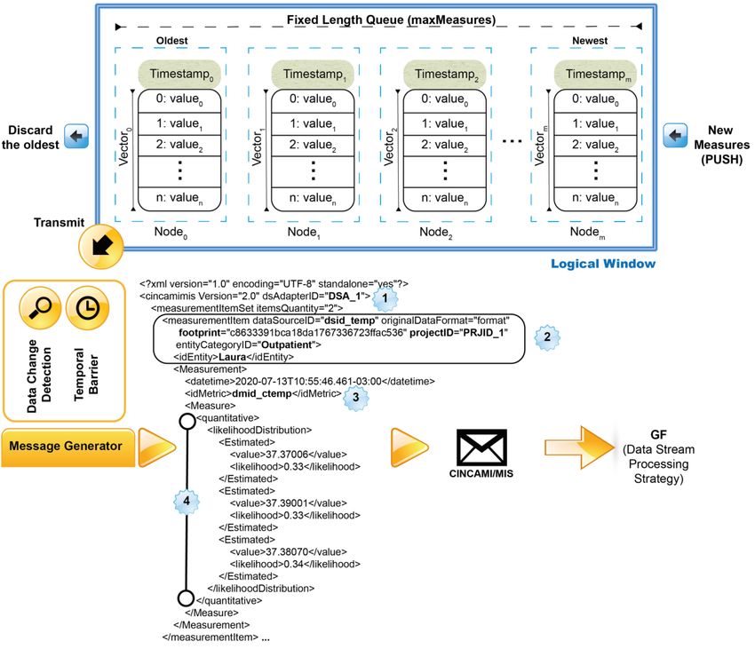
International Journal of Mathematical, Engineering and Management Sciences
Vol. 6, No. 1, 363-382, 2021
https://doi.org/10.33889/IJMEMS.2021.6.1.023

Figure 1 synthesizes the organization and global behavior of the data buffer. The data buffer in the
MA is organized as a logical window with an arbitrary capacity that is defined using a parameter
maxMeasures. Each time that sensors inform measures, they are added chronologically into the
data buffer incorporating the timestamp and keeping the order given by the paired metrics (e.g., the
position 0 corresponds to the value of the corporal temperature and so on). When the data buffer
reaches the defined limit, the oldest data vector (i.e., the left extreme in Figure 1) will be discarded
to be replaced by the newest (i.e., the right extreme in Figure 1). In this way, the data buffer seems
to be unlimited, but indeed, it keeps the last measures related to sensors based on the value
established for the maxMeasures parameter.

 Figure 1. A conceptual perspective of the data buffer and the measurement interchange schema.

The data buffer keeps the last measures in memory waiting for a signal to transmit them. This signal
could have an origin from two different points of view 1) A data change detection: each metric has
an online filter implemented following the approach of (Cao and Rhinehart, 1997; Alford et al.,
2018) which allows informing when there is enough proof that a data change has occurred, or 2) A
temporal barrier: it establishes a minimum timespan through which at least one data transmission
should be made. This is a complement to the data change detection because when no data change

 368

International Journal of Mathematical, Engineering and Management Sciences
Vol. 6, No. 1, 363-382, 2021
https://doi.org/10.33889/IJMEMS.2021.6.1.023

is detected for a given time, the temporal barrier will transmit the current data in the buffer to
provide a proof-of-life. This articulation allows implementing a smart data transmission strategy,
avoiding continuous data transmission, and fostering a rational use of resources.

When the transmission signal is originated from an active detector (no matter whether it was
originated by the temporal barrier or a data change detection), the data buffer content is structured
under the CINCAMI/Measurement Interchange Schema -CINCAMI/MIS-(Diván and Sánchez
Reynoso, 2020b) to be transmitted immediately to the Gathering Function at DSPS. Each
CINCAMI/MIS message is generated based on the CINCAMI/PD project definition which allowed
structuring the data buffer. From the project definition, information about the entity ID, data source
ID, metric ID, the kind of expected value (e.g., estimated or deterministic), among other aspects is
obtained to be incorporated in the messages with measures. Because the project definition could
consider complementary data (e.g., the geographic positioning related to a measure), each
CINCAMI/MIS message could structurally vary according to whether it informs complementary
data or not.

As it is possible to appreciate in Figure 1, each CINCAMIMIS message contains data (i.e.,
measures) but also metadata (i.e., tags) describing the meaning based on the measurement project
definition. Each tag jointly with its corresponding IDs allows DSPS to interpret the measure
contained in each CINCAMI/MIS message in its corresponding context. For example, the
“dsAdapterID” tag indicates a specific MA acting as the message’s origin jointly with the version
of it (See the star with 1 in Figure 1). The rectangle associated with the star 2 indicates the ID for
the origin’s sensor (e.g., dsid_temp), a footprint to verify the measure content, the associated project
ID (e.g., PRJID_1), and the associated entity category (e.g., Outpatient). The star with 3 in Figure
1 explicitly indicates the associated metric (e.g., dmid_ctemp) with the values specified in the star
with 4, which in the example are associated with a likelihood distribution (alternatively, it could be
a single deterministic value too). For that reason, when GF receives a CINCAMIMIS message
knows the way to process each value due to each ID allows looking up the associated definition for
its interpreting.

 − ̅
 = (1)
 
As it is possible to appreciate in equation (1), to reach a Z-score, it is necessary to estimate at least
the arithmetic mean and standard deviation (i.e., ̅ and s respectively), but the data buffer is
continuously receiving data from sensors while it discards the oldest ones. For such a reason, an
incremental strategy to estimate each one is necessary.

 ̅ −1 ∗ −1 + 
 ̅ = (2)
 −1 + 1
Equation (2) provides a simple way to update continuously the arithmetic mean each time that a
new measure arrives. It obtains the original sum through the product between the current arithmetic
mean (i.e., ̅ −1 ) with the current number of processed measures (i.e., −1 ). Such a product is
added to the new received measure (i.e., ̅ ) and the result is divided by −1 plus one.

The standard deviation in a “t” time is estimated through the sample variance using equation (3).
In this sense, it is important to highlight that the estimation uses the current arithmetic mean

 369

International Journal of Mathematical, Engineering and Management Sciences
Vol. 6, No. 1, 363-382, 2021
https://doi.org/10.33889/IJMEMS.2021.6.1.023

available at the time in which the measure has arrived.

 ∑ =1( − ̅ )2
 = √ (3)
 −1
Equation (4) schematizes this situation, where the arithmetic average for each time is not
necessarily equal to the predecessor or successor due to the updating associated with each arrived
value according to equation (2).

 ( 1 − ̅1 )2 + ( 2 − ̅2 )2 + ( 3 − ̅3 )2 + ( 4 − ̅4 )2
 4 = √ (4)
 4−1
The implementation of equations (3) and (4) require keeping in memory the accumulators jointly
with the number of processed measures. However, it was said that the logical window will discard
the oldest data vectors to retain the new ones, and such an action will affect equations (2), (3), and
(4) because a part of the sum of equation (2) or the difference between the measure and its
arithmetic average in equations (3) and (4) will be discarded. To avoid this situation, equations (5)
and (6) are fitted as follows supposing a maxMeasures parameter with a value of 100.

 ̅ −1 ∗ −1 + − −100
 ̅ = (5)
 −1 + 1 − 1
Equation (5) rests the value to be discarded (i.e., −100) and at the same time it discounts in 1 the
divisor, while the new value is incorporated (i.e., ).

 (∑ =1( − ̅ )2 ) − ( −100 − ̅ −100 )2
 = √ (6)
 −1−1
Something similar to equation (5) occurs in equation (6). The difference related to the oldest data
vector to be discarded (i.e., ( −100 − ̅ −100 )) is decreased from the accumulator at the time the
new difference is incorporated. The divisor is decreased in 1 but n is parallelly increased by the
new measure, having as a limit the maxMeasures parameter (i.e., ≤ ). The
implementation of equation (6) requires that for each data vector in memory, the estimated
arithmetic average in a given instant be jointly stored to process the eventual discarding after.

Alternatively, equation (7) proposes an option to equation (6) to obtain incrementally the variance
without needs to keep the accumulators in memory. This alternative requires to know the previous
deviation estimation, the previous arithmetic average estimation, and the number of observations.
However, even when they look similar, they have a conceptual difference. On the one hand,
equation (6) goes progressively fitting its value according to the last “100” data vectors in
consonance with the arithmetic average estimation (See equation (5)), allowing a better
characterization of it. On the other hand, equation (7) goes estimating the variance from the
beginning of the data series and not based on the last values.

 2
 ( − ̅ −1 )2
 = √ ∗ [ −1 + ] (7)
 +1 +1

 370

International Journal of Mathematical, Engineering and Management Sciences
Vol. 6, No. 1, 363-382, 2021
https://doi.org/10.33889/IJMEMS.2021.6.1.023

Thus, equation (7) would be a better alternative to study the whole deviation estimation when it is
required. However, equation (6) would be a better choice option when the partial sum needs to be
used to estimate the covariances among metrics and the deviation should be explicative of the data
contained in the data buffer as occurs here.

Let “i” and “j” two metrics to be implemented in a MA, the covariance between them could be
calculated using equation (7) based on equation (6) as follows.

 [∑( − ̅ ) ∗ ( − ̅ )] − [( −100 − ̅ −100 ) ∗ ( −100 − ̅ −100 )]
 ( , ) = (8)
 −1−1
Equation (8) would require keeping in memory the differences to subtract them when the data
vector is discarded. Thus, given a number m of metrics and utilizing equation (8), it is possible to
approach the covariance matrix incrementally according to the logical window as it is indicated in
equation (9).

 21 … 1 
 = [ … … … ] (9)
 1 … 2 

The covariance matrix described by equation (9) is triangular because ( , ) = ( , ). This
allows implementing as a unidimensional array mapping the elements according to a triangular
matrix, optimizing the use of memory. Also, from equation (8), it is possible to get Pearson’s
correlation matrix as it is indicated in equation (10).

 ( , ) ( , )
 ∀ ≠ : , = =
 √ ( , ) ∗ √ ( , ) ∗ 
 (10)
 ( , ) 2 
 ∀ = : , = = =1
 { √ ( , ) ∗ √ ( , ) ∗ 

The library pabmmCommons library is available on GitHub
(https://github.com/mjdivan/pabmmCommons) and it incorporates the object model described by
Figure 2 jointly with the implementation of the mentioned formulas and data buffer for the real-
time data processing. The library is written in Java 8 and it was released under the terms of the
Apache 2.0 license.

Figure 2 highlights with yellow background the new classes incorporated in the pabmmCommons
library. The SPCMeansBasedNode class is a specialization of the SPCBasedBufferNode class with
the possibility to keep the estimated arithmetic averages and differences with the measures
concurrently in memory under the same node into the data buffer.

The SPCMeansBasedBuffer class implements incremental computing of arithmetic averages and
variances when the data vector with measures is incorporated. This class is a specialization of
SPCBasedBuffer class that keeps in memory a logical window implemented through a concurrent
linked queue of SPCMeansBasedNode instances. The class implements the Observer interface to
monitor the online data change detectors and know when a data change has occurred. Also, it
extends the Observable class to inform to the message generator (See Figure 1) that a new data

 371

International Journal of Mathematical, Engineering and Management Sciences
Vol. 6, No. 1, 363-382, 2021
https://doi.org/10.33889/IJMEMS.2021.6.1.023

transmission could be carried forward, be it as a consequence of a temporal barrier or the data
change detectors.

 Figure 2. Main classes related to the data buffer with the capacity of estimating incrementally.

The SimilarityTriangularMatrix class implements a triangular matrix through the mapping from/to
a unidimensional array. The IncrementalCovMatrix class implements the computing for the
incremental covariance and correlation matrixes, using an instance of the
SimilarityTriangularMatrix class to manage data in memory. When a data transmission is
performed, the data buffer is cleaned, and all the estimations will be restarted again.

The attributes deviationLimit, acceptanceThreshold, and loadShedding are directly associated with
the application of the load-shedding technique that is detailed then.

4. A Metadata and Z Score-based Load-Shedding Technique
From the estimation of the arithmetic averages and standard deviations for each metric, it is possible
to get the Z-scores which are especially useful to avoid the effect of variables with great magnitude
in detriment of those with a different variation range. The set of variables (or metrics) managed to
a measurement adapter is established in the measurement project definition, which is paired with
sensors during the startup. The metadata is associated with the data buffer, where it is possible to

 372

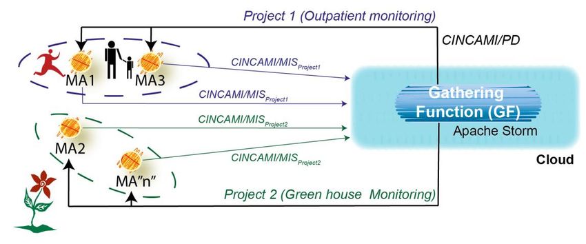
International Journal of Mathematical, Engineering and Management Sciences
Vol. 6, No. 1, 363-382, 2021
https://doi.org/10.33889/IJMEMS.2021.6.1.023

appreciate the set of metrics managed (See the metID attribute in the SPCBasedBuffer class) jointly
with its weightings (See the weighting attribute in the SPCBasedBuffer class). The weighting
expresses the relative importance of each metric in the measurement project and it is defined by the
project director. When the loadShedding attribute in the SPCMeansBasedBuffer class is established
to false (it is the default value), the data buffer will transmit data following two complementary
policies. On the one hand, when an online filter informs that a data change has occurred. On the
other hand, when a temporal barrier indicates that transmission must be done as a proof-of-life
because it has elapsed a certain time without any transmission. Each time that an online filter is
triggered indicating a data change, the temporal barrier is restarted to zero. The last one only is
triggered when there not exists a data transmission after a certain time (15 seconds by default).

Previously, DSPS only applied the load-shedding technique in GF but when it was applied, the data
have already been transmitted and they were discarded in GF. That is to say, GF is the architectural
receiver of all measures coming from a certain number of heterogeneous measurement adapters.
All of them are physically located at different points with autonomous behavior. For example,
Figure 3 conceptually describes two different measurement projects. On the one hand, project 1 is
related to the outpatient monitoring and each MA is related to a given outpatient under monitoring.
On the other hand, project 2 refers to a greenhouse monitoring where MA2 and MA”n” monitor
different locations. In this sense, some considerations are worthy to be highlighted 1) Project 1 and
2 are initialized using the corresponding project definition through the CINCAMI/PD message, 2)
The CINCAMIPD message between project 1 and 2 are structurally different because their aims
are completely different, 3) The CINCAMI/MIS related to project 1 and 2 are structurally different.
In the same project, the informed measures from measurement adapters will be conceptually
different because they are monitoring different entities (though structurally similar), 4) GF takes
knowledge from collected measures once each CINCAMI/MIS message has been transmitted
through the Internet using the Cloud and not before, 5) GF receives simultaneously CINCAMIMIS
messages from different MA associated with different projects, 6) From the MA perspective, the
processing rate of GF is unknown, and 7) GF could send a message to each MA but not manage its
data processing.

 Figure 3. Conceptual description of the location of GF and MA and its impact on the data transmission.

Thus, the idea is to complement to GF with a local load shedding implemented on the MA before
the data transmission is performed. Thus, when GF is close to reaching a risky processing rate

 373

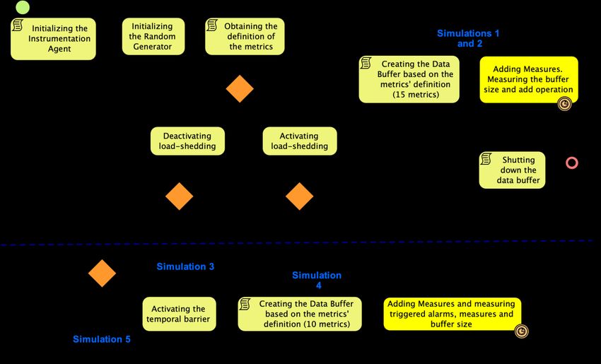
International Journal of Mathematical, Engineering and Management Sciences
Vol. 6, No. 1, 363-382, 2021
https://doi.org/10.33889/IJMEMS.2021.6.1.023

according to (Diván and Sánchez Reynoso, 2020a), it could request to MA that the local load-
shedding techniques need to be activated through the activation of the loadShedding flag from the
SPCMeansBasedBuffer class. This will imply that MA will filter the data to be retained in the buffer
using equation (11), while only will perform data transmissions when a data change is detected,
discarding any intent of data transmission as a proof-of-life.
 
 ∑ ⃗ ∗ 
 ⃗⃗⃗ < ℎ ℎ (11)
 =1

Equation (11) describes the data retention policy of each MA based on an acceptanceThreshold
parameter which is indicated in each project definition. The vector ⃗ is the Z-score vector
computed from the estimation of the arithmetic average and the deviation for each metric. The
vector 
 ⃗⃗⃗ contains the weighting of each metric defined in the project definition to know the relative
importance of each one. Thus, the joint measures from sensors will be retained in the data buffer
when the product does not exceed the established threshold, otherwise, the measures are discarded
because the focus is applied to the general behavior and not in outliers throughout the period where
the load-shedding technique is enabled.

Thus, when a data vector is received, it is standardized using the estimations for the average and
standard deviation. When the Z-score of a variable individually exceeds the deviation limit (See
the deviationLimit attribute in the SPCMeansBasedBuffer class, it has a value of 2 by default), it
will be accumulated multiplying it by its corresponding weighting. In the end, the data vector will
be retained in the data buffer when the cumulated sum of the product between Z-scores and
weightings do not exceed the acceptance threshold (See the acceptanceThreshold attribute in the
SPCMeansBasedBuffer class, it has a value of 3 by default).

This kind of filtering strategy is dynamical because the estimations go updating continuously on
each new data vector, and the fact of discard an excessive variation is related to study the general
behavior instead of the outlier itself. The metric’s metadata allows knowing the relative importance
of each variable in the project to decide to retain a given data vector.

In this way, only the data following the general behavior about updated estimators are retained in
the data buffer, while the message generator will inform data from MA only when a data change
has occurred. An analysis of discrete simulations based on the number of data transmissions and
associated resources with the data buffer are outlined in the next sections to provide some initial
applicability patterns.

The possibility to incorporate the covariance and correlation matrix allows detecting dependencies
between variables, leaving as a future work other kinds of dependences analysis jointly with its
impact on the acceptance/rejection policies related to online filters.

5. Discrete Simulations on the Data Buffer: Methodological and Quantitative Points
of View
Four discrete simulations were scheduled to provide initial applicability patterns about the proposed
updates in the pabmmCommons library. All simulations have a common region related to the
initialization of the Java Instrumentation Agent to measure the runtime memory consumption and
the initialization of a numbers’ random generator jointly with the loading of a measurement project

 374

International Journal of Mathematical, Engineering and Management Sciences
Vol. 6, No. 1, 363-382, 2021
https://doi.org/10.33889/IJMEMS.2021.6.1.023

containing 10 metrics. The metrics’ information based on whether the load-shedding technique is
activated or not will derivate in a given initialization of the data buffer according to the chosen
simulation.

All simulations were performed on a MacBook Pro running macOS Catalina 10.15.5 with a 2,9
GHz Intel Core i7 processor, 16GB 2133 MHz LPDDR3 of RAM, and a Radeon Pro 560 4GB of
dedicated RAM. It was used Netbeans 9 on Java 8 (A runtime environment version 1.8.0_191) on
a 64-bit platform. A BPMN diagram detailing the simulations’ steps is synthesized in Figure 4.

 Figure 4. A BPMN diagram describing the discrete simulation methodology.

Simulations 1 and 2 were oriented to measure the add operation in the data buffer when the load-
shedding technique is enabled (i.e., the simulation 2), or when it is disabled (i.e., the simulation 1).
Both simulations ran for 5 minutes, incorporating each 100 ms a data vector randomly generated
(With an arithmetic average of 35 and a standard deviation of 2) in the data buffer. The vector
dimensionality was associated with 15 metrics, while the data buffer was defined to retain 1000
data vectors. Once the data vector had been incorporated, measures about the required time and the
current size of the data buffer are updated through the console.

Simulations 3, 4 and 5 were oriented to analyze the behavior of the triggered alarms for data
transmission from the data buffer. Simulation 3 describes the behavior when the load-shedding
technique is disabled, making the data transmissions based on the online filter and temporal barrier
(i.e., as a proof-of-life). Simulation 4 details the behavior with the load-shedding technique enabled
and deactivating the temporal barrier. When the load-shedding is enabled the only considered alarm
to perform a data transmission is based on the online filter detecting data changes, for such a reason
the simulation time was increased up to 15 minutes monitoring concurrently 10 metrics, keeping
the logical window with a capacity of retaining the last 1000 data vectors. Simulation 5 exposes a

 375

International Journal of Mathematical, Engineering and Management Sciences
Vol. 6, No. 1, 363-382, 2021
https://doi.org/10.33889/IJMEMS.2021.6.1.023

scenario where the load-shedding technique is disabled jointly with the temporal barrier, the
transmissions are performed based on the online filter considering all data (i.e., no data discarding
is allowed), while the estimation of arithmetic means and deviations of metrics is performed online
using an instance of the SPCMeansBasedBuffer class.

As it is shown in Figure 4, once the simulations 1, 2, 3, or 4 reach the end, the data buffer is shut
down, releasing the reserved resources, and ending the program. The implementations of these
discrete simulations are available in the mainMeansBufferDetectors class in the
org.ciedayap.simula package.

 20 1.000
 890,26
 18,61
 18 900

 16 800

 14 700
 Total Operation Time (ms)

 12 600

 Size (KB)
 10 500

 8 400

 6 300

 4 200

 2 100

 0 0
 0
 6
 11
 17
 23
 28
 34
 40
 45
 51
 57
 63
 69
 75
 80
 86
 92
 98
 104
 110
 116
 122
 128
 134
 140
 146
 152
 158
 164
 170
 176
 182
 188
 194
 200
 206
 212
 218
 224
 230
 236
 242
 248
 254
 260
 266
 272
 278
 285
 291
 297
 Elapsed Time (seconds)

 addTime (ms) addTimeLS (ms) Data Buffer Size (KB)

Figure 5. Evolution of the operation time and data buffer size throughout 5 minutes (Simulations 1 and 2).

Figure 5 shows the evolution of the “add” operation time jointly with the data buffer size when the
load-shedding option is enabled (i.e., the simulation 2 which is identified with orange color), and
when it is disabled (i.e., the simulation 1 which is identified with the blue color). The operation
time is quantified using the left ordinate axis, while the size expressed in Kilobytes is represented
on the right ordinate axis of the figure. The outliers are a consequence of Java’s garbage collector
that was operating while the simulation was performed. Independently of them, it is possible to
appreciate that the “add” operation has a similar behavior though some differences could be
highlighted in the boxplot in Figure 6. When the Load-Shedding (LS) technique was enabled, the
“add” operation time through the data discarding was subtle better, reaching an arithmetic average
of 0.49 ms and a median of 0.44 versus 0.62 ms and 0.54 ms when the LS was disabled. Also, the
variation range was regulated when LS was enabled as it is possible to appreciate through the
boxplot in Figure 6, which is consistent with their standard deviations obtained (i.e., 0.51 when LS

 376

International Journal of Mathematical, Engineering and Management Sciences
Vol. 6, No. 1, 363-382, 2021
https://doi.org/10.33889/IJMEMS.2021.6.1.023

is enabled versus 0.31 when it is disabled). Thus, the use of LS technique decreases in 0.1 ms the
individual operation time considering its median, which represents an initial optimization of
22.72% (i.e., [[0.54/0.44]-1]*100).

 1,60

 1,40

 Total Operation Time (ms) 1,20

 1,00

 0,80

 0,60

 0,40

 0,20

 0,00
 addTime (ms) addTimeLS (ms)

 Figure 6. Boxplot for the addTime operation (without and with the Load-shedding enabled) throughout 5
 minutes considering the measures under 2 ms for better visibility (Simulations 1 and 2).

Also, even when the LS technique is running in parallel, the logical window allows keeping stable
the data buffer size, which can be appreciated in Figure 5. Once the logical window reaches the
max occupation (i.e., 1000 data vectors in these simulations), it starts to discard the oldest data
vectors to retain the new ones, keeping stable the data buffer size in 890,26 Kb for 10 metrics. The
possibility of articulating the LS technique with a logical window in the data buffer allows retaining
data that vary according to the most important metrics indicated in the project definition, avoiding
an overhead in the “add” operation time.

However, the outlier introduces a temporal limitation about the applicability of the LS technique in
conjunction with the data buffer based on a logical window. These incremental estimations are
possible if and only if the time between data arriving is upper than 18,61 ms. In the best case and
scenario, this operation time could be reduced to 0.08 ms. Also, it is important to indicate that a
data buffer monitoring concurrently 10 metrics with 1000 available slots (i.e., up to 10,000
measures) would require 890,26 KB to store all information related to the data buffer and LS
techniques.
Figure 7 describes the shown behavior by the number of triggered alarms and the volume of data
transmissions throughout 15 minutes of simulation with the load-shedding technique disabled. The

 377

International Journal of Mathematical, Engineering and Management Sciences
Vol. 6, No. 1, 363-382, 2021
https://doi.org/10.33889/IJMEMS.2021.6.1.023

left ordinate axis indicates the number of triggered alarms, while the right ordinate axis indicates
the number of slots (i.e., each slot contains a full data vector with all its variables) transmitted as a
consequence of the triggered alarm. As it is possible to appreciate, the alarms triggered due to a
temporal barrier are indicated with the blue color, while those related to a data change are
represented with the orange color. Numbers over the bar describe the accumulated number of
triggered alarms of such a type, for example, the last bar on the right side indicates 51 alarms with
an origin in the temporal barrier and 8 related to a data change. That is to say, from 59 alarms in
the 15 minutes, 86,44% corresponds to a temporal barrier in which it aims to provide a proof-of-
life to GF. Just 13,56% of the data transmission is associated with data change.

 60 256
 250
 238
 231 8
 225 8
 8
 8
 50 8 8
 8
 8 200
 8
 8 8
 8
 8

 Number of Transmitted Slots
 8
 40 8
 169
 8 8
#Triggered Alarms

 157 8
 148 8
 137 137 7 7 150
 145 7
 7
 137 137 137 137 136 6 7 136 137 137 136 136 137 136
 30 128 6
 125 6
 6
 116 6 6
 6 51
 104 5 5 49 50
 5 47 48 100
 5 44 45 46
 5 41 42 43
 20 5 39 40
 5
 5 37 38
 5 34 35 36
 4 5 31 32 3333
 4 2929 30
 4 27 28
 4 24 25 26
 49 4 50
 22 23
 10 4 4 19 20
 21
 3 4 16 17 18 42 34
 3 1414 15
 3 12 13
 3 10 11
 2 3 8 9 17
 2 5 6 7 7
 1 2 3 3 4
 0 1 1 1 2 0
 6

 8

 8
 69

 41

 71

 72

 73

 71

 75

 76

 77

 78

 33

 80

 81

 82

 83

 84

 63

 86

 87

 88

 89

 90

 91

 92

 93

 94
 ,0

 ,6

 ,6
 -

 9,

 7,

 9,

 9,

 9,

 8,

 9,

 9,

 9,

 9,

 9,

 9,

 9,

 9,

 9,

 9,

 8,

 9,

 9,

 9,

 9,

 9,

 9,

 9,

 9,

 9,
 36

 69

 99
 12

 15

 18

 21

 24

 27

 30

 33

 36

 39

 41

 45

 48

 51

 54

 57

 59

 63

 66

 69

 72

 75

 78

 81

 84

 87
 Elapsed Time (seconds)

 #Triggered Alarms #Temporal Barrier Alarms #Data Change Alarms #records

 Figure 7. Evolution of the triggered alarms and data transmissions throughout 15 minutes (simulation 3).

Independently of the data transmission origin, an average of 136 slots are informed in each
operation which represents around 1360 measures (i.e., 10 metrics * 136 measure/metrics). The
minimum volume of informed data was 17 slots (i.e., 170 measures) consuming 14,26 KB, while
the maximum volume was 256 slots (i.e., 2560 measures) consuming 117,88 KB.

Figure 8 describes the exposed behavior throughout 15 minutes of simulation with the load-
shedding technique enabled. The left ordinate axis indicates the number of triggered alarms, while
the right ordinate axis indicates the number of slots (i.e., each slot contains a full data vector with
all its variables) transmitted as a consequence of the triggered alarm. Results seem to be promising
because just 15 data transmissions were required for 15 minutes versus the 59 required without the
technique. This avoids around 74.57% of data transmissions, consuming the resources associated
with 25.43% of the original transmissions. Also, the volume of informed data has changed. When
the technique is activated, the maximum number of transmitted data was 999 slots (i.e., 9990
measures) consuming 440.05 KB, while the minimum number was 44 slots (i.e., 440 measures)
consuming 25,96 KB. As it was introduced, all the alarms in this simulation are associated with

 378

International Journal of Mathematical, Engineering and Management Sciences
Vol. 6, No. 1, 363-382, 2021
https://doi.org/10.33889/IJMEMS.2021.6.1.023

data changes detected through the online filters based on data that were retained accordingly with
the Z-scores and the weightings of the defined metrics. Any kind of temporal barrier is deactivated
when the load-shedding technique is enabled.
 20 1200

 999 999 1000

 15

 800

 Number of Transmitted Slots
 759
 #Triggered Alarms

 10 654 600
 551 555

 416 15
 14
 13 400
 356 12
 324 11
 5 10
 287 285
 9
 239 8 253
 7 200
 6
 5
 4
 3
 2
 1 44
 0 0 0 0 0 0 0 0 0 0 0 0 0 0 0 0
 - 35,14 61,07 121,73 236,84 268,05 306,80 378,70 424,63 508,47 569,97 601,40 629,14 762,42 871,32
 Elapsed Time (seconds)

 #Temporal Barrier Alarms #Data Change Alarms #records

 Figure 8. Evolution of the triggered alarms and data transmissions throughout 15 minutes with load-
 shedding technique enabled (simulation 4).

 20 1200

 1000
 953
 15

 800
 770
 Number of Transmitted Slots

 748
 699
 #Triggered Alarms

 628
 10 600
 564

 446
 506 15
 419 14
 13 400
 12
 344 346 347
 323 11
 5 10
 9
 239 8
 7 200
 6
 5
 4
 3
 59 2
 1
 0 0 0 0 0 0 0 0 0 0 0 0 0 0 0 0
 - 25,65 60,22 97,27 158,28 203,30 240,30 295,35 343,24 418,90 486,79 568,12 651,78 689,11 793,36
 Elapsed Time (seconds)

 #Temporal Barrier Alarms #Data Change Alarms #records

 Figure 9. Evolution of the triggered alarms and data transmissions with the load-shedding technique and
 temporal barrier disabled (Simulation 5).

 379

International Journal of Mathematical, Engineering and Management Sciences
Vol. 6, No. 1, 363-382, 2021
https://doi.org/10.33889/IJMEMS.2021.6.1.023

Figure 9 describes the exposed behavior throughout 15 minutes of simulation with the load-
shedding technique and proof-of-life disabled but computing the estimation for arithmetic average
and deviations. The online filter is used to detect data changes and transmit accordingly.
Analogously with Figure 8, the left ordinate axis indicates the number of triggered alarms, while
the right ordinate axis indicates the number of slots (i.e., each slot contains a full data vector with
all its variables) transmitted as a consequence of the triggered alarm. Comparing Figures 8 and 9,
it is possible to appreciate that even when the number of data transmissions is the same, the load-
shedding technique (See Figure 8) incorporates a delay to transmit. That is to say, reading from the
second transmission’s time onward in both figures, it is possible to appreciate a subtle delay when
load-shedding is enabled, for example, the transmission 2 in Figure 9 occurred at 25,65 seconds
while in Figure 8 at 35,14 seconds, the transmission 10 in Figure 9 was made at 418,9 seconds
while in Figure 8 at 508,47 seconds, and in this way so on. The average time between transmissions
is 57,67 seconds with the load-shedding disabled with a median of 446 slots by transmission, while
it is 62,24 seconds with a median of 416 slots by transmission when the technique is enabled. For
that reason, it would be probable that the number of transmissions with load-shedding disabled is
higher when the considered period is higher than 15 minutes.

However, this result is interesting because if for any reason the load-shedding do not want to be
used (e.g., to avoid discarding data), data transmissions limited to proof-of-life allow
complementing to GF in front of an eventual overhead with similar results, keeping active the
online estimation of the arithmetic averages and deviations.

6. Conclusions
This work has introduced a Metadata and Z-score based load-shedding technique in the
measurement adapter articulated with a data buffer that implements a logical window behavior in
the DSPS. The capacity to retain a given volume of data avoiding an overflow allows waiting for
the precise instant to perform data transmission. Also, while the data are incorporated in the data
buffer, an incremental strategy to estimate the arithmetic average, standard deviations, covariance,
and correlations were introduced. Thus, such estimations were used to implement the data retention
policy that is supported by the weightings coming from the measurement project to discriminate
among different levels of importance for the metrics. Discrete simulations indicated that a
minimum of 18.61 ms between data arriving from sensors is necessary to process the data in the
buffer, while 890,26 KB was required to implement it.

It is worthy to mention the saving of resources generated by the load-shedding technique. In a
normal situation, MA will transmit around 59 times (51 emerged from temporal barriers and 8 from
data change detections) with 136 slots as average in each transmitted message. In contrast with it,
with the load-shedding technique activated, MA only required 15 data transmissions increasing to
513 slots the average of data to be transmitted by each message. This represented a saving of around
74% in comparison to the original data transmissions, which is very interesting not only for the MA
but also for the GF because now it is possible to request collaboration to MA to discard data before
they are sent. That is to say, when the processing rate of GF is close to being exceeded, it could
activate its global load-shedding technique and also it notifies to each MA to activate the local LS.
Thus, this distributed behavior could decrease the data volume received by GF up to 74%, allowing
release resources and to solve the potential bottleneck in the DSPS. Simulation 5 showed an
interesting alternative when no data want to be discarded. The alternative uses the online data filter
to regulate the data transmissions, avoiding the temporal barriers, and computing in real-time the
estimations about arithmetic averages and deviations, reaching similar results to the use of the load-

 380

International Journal of Mathematical, Engineering and Management Sciences
Vol. 6, No. 1, 363-382, 2021
https://doi.org/10.33889/IJMEMS.2021.6.1.023

shedding technique. However, the time between transmissions is lower than when the load shedding
is used.

Thus, this approach would be feasible to be applied on a given device if device were able to manage
a volume of 2MB of RAM (i.e., 1MB for the data buffer and load-shedding technique, while another
equal is necessary to prepare the data message to be transmitted) it is warrantied a lifespan of at
least 19 ms between each arrived data.

All the source code related to the pabmmCommons library for the extensions detailed jointly with
the corresponding simulations here described are freely available on GitHub for your reference.

As future work, other kinds of dependencies analysis jointly with its impact on the data
acceptance/rejection policies related to online filters will be analyzed.

Conflict of Interest
The authors confirm that there is no conflict of interest to declare for this publication.

Acknowledgment
This research is partially supported by the project CD 312/18 from the Economy School at the National University of La
Pampa.

References
Alford, J.S., Hrankowsky, B.M., & Rhinehart, R.R. (2018). Data filtering in process automation
 systems. InTech, 65(4), 14-19.
Cao, S., & Rhinehart, R.R. (1997). A self-tuning filter. Journal of Process Control, 7(2), 139-148.
Cardellini, V., Mencagli, G., Talia, D., & Torquati, M. (2019). New landscapes of the data stream
 processing in the era of fog computing. Future Generation Computer Systems, 99, 646-650.
Chen, Y., Li, M., Chen, P., & Xia, S. (2019). Survey of cross-technology communication for IoT
 heterogeneous devices. IET Communications, 13(12), 1709-1720.
Diván, M.J., & Sánchez Reynoso, M.L. (2020a). A load-shedding technique based on the
 measurement project definition. In: Jain, V., Patnaik, S., Popențiu Vlădicescu, F., Sethi, I. (eds)
 Recent Trends in Intelligent Computing, Communication and Devices. Springer, Singapore,
 1006, pp. 1027-1033.
Diván, M.J., & Sánchez Reynoso, M.L. (2020b). An architecture for the real-time data stream
 monitoring in IoT. In: Tanwar, S., Tyagi, S., Kumar, N. (eds) Multimedia Big Data Computing
 for IoT Applications. Springer, Singapore, 163, pp. 59-100.
Fernández-Rodríguez, J.Y., Álvarez-García, J.A., Fisteus, J.A., Luaces, M.R., & Magaña, V.C.
 (2017). Benchmarking real-time vehicle data streaming models for a smart city. Information
 Systems, 72, 62-76.
Ghobaei-Arani, M., Souri, A., & Rahmanian, A.A. (2020). Resource management approaches in
 fog computing: A comprehensive review. Journal of Grid Computing, 18, 1-42.

 381