Time-lagged Independent Component Analysis of Random Walks and Protein Dynamics
←
→
Page content transcription
If your browser does not render page correctly, please read the page content below
bioRxiv preprint doi: https://doi.org/10.1101/2021.03.18.435940; this version posted March 18, 2021. The copyright holder for this preprint
(which was not certified by peer review) is the author/funder, who has granted bioRxiv a license to display the preprint in perpetuity. It is made
                                            available under aCC-BY-NC-ND 4.0 International license.

             Time-lagged Independent Component Analysis of
                 Random Walks and Protein Dynamics

                                Steffen Schultze1                                 Helmut Grubmüller1
                            sschult@mpibpc.mpg.de                                  hgrubmu@gwdg.de

                             1
                                 Max Planck Institute for Biophysical Chemistry
                                                            March 18, 2021

                                                                  Abstract

                 Time-lagged independent component analysis (tICA) is a widely used dimension
             reduction method for the analysis of molecular dynamics (MD) trajectories and has
             proven particularly useful for the construction of protein dynamics Markov models.
             It identifies those ’slow’ collective degrees of freedom onto which the projections of
             a given trajectory show maximal autocorrelation for a given lag time. Here we ask
             how much information on the actual protein dynamics and, in particular, the free
             energy landscape that governs these dynamics the tICA-projections of MD-trajectories
             contain, as opposed to noise due to the inherently stochastic nature of each trajectory.
             To answer this question, we have analyzed the tICA-projections of high dimensional
             random walks using a combination of analytical and numerical methods. We find that
             the projections resemble cosine functions and strongly depend on the lag time, exhibiting
             strikingly complex behaviour. In particular, and contrary to previous studies of principal
             component projections, the projections change non-continuously with increasing lag time.
             The tICA-projections of selected 1 µs protein trajectories and those of random walks
             are strikingly similar, particularly for larger proteins, suggesting that these trajectories
             contain only little information on the energy landscape that governs the actual protein
             dynamics. Further the tICA-projections of random walks show clusters very similar
             to those observed for the protein trajectories, suggesting that clusters in the tICA-
             projections of protein trajectories do not necessarily reflect local minima in the free
             energy landscape. We also conclude that, in addition to the previous finding that certain
             ensemble properties of non-converged protein trajectories resemble those of random
             walks, this is also true for their time correlations. Due to the higher complexity of
             the latter, this result also suggests tICA analyses as a more sensitive tool to test MD
             simulations for proper convergence.

                                                                        1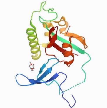
bioRxiv preprint doi: https://doi.org/10.1101/2021.03.18.435940; this version posted March 18, 2021. The copyright holder for this preprint
(which was not certified by peer review) is the author/funder, who has granted bioRxiv a license to display the preprint in perpetuity. It is made
                                            available under aCC-BY-NC-ND 4.0 International license.

     1       Introduction
    The atomistic dynamics of proteins, protein complexes, and other biomolecules is exceedingly
    complex, covering time scales from sub-picoseconds to up to hours [1, 2]. It is governed by a
    similarly complex high-dimensional free energy landscape or funnel [3], characterized by a
    hierarchy of free energy barriers [4], and has been widely studied computationally by molecular
    dynamics (MD) simulations [5]. With particle numbers ranging from several hundreds to
    hundreds of thousands or more [6, 7, 8, 9], the correspondingly high-dimensional configuration
    space of the system poses considerable challenges to a fundamental understanding of biomolec-
    ular function, e.g., of the conformational motions of these biological ‘nano-machines’ [10, 11],
    protein folding [12], or specific binding.
     Several attempts to reduce the dimensionality of the dynamics have addressed this issue.
     Most notable approaches are principal component analysis (PCA) to extract the essential
     dynamics [13] of the protein that contributes most to the atomic fluctuations, and time-lagged
     independent component analysis (tICA), which identifies those collective degrees of freedom
     that exhibit the strongest time-correlations for a given lag-time [14, 15]. Both dimension
     reduction techniques can yield information on the conformational dynamics of a protein, i.e.,
     how the protein moves through several conformational substates, which can be defined as
     metastable conformations characterized by local free energy minima [16].
    This property also renders these dimension reduction techniques highly useful as a pre-
    processing step to describing the conformational dynamics of macromolecules in terms of a
    discrete Markov process [17, 18, 19]. Currently tICA is most widely used, and it is preferred
    over PCA for this purpose [20] because it additionally uses time information of the input
    trajectory.
     In this context, both PCA and tICA rely on MD trajectories as input, which raises the
     question how much of these analyses is determined by actual information on the protein
     dynamics, as opposed to noise due to the inherently stochastic nature of each trajectory, and,
     importantly, how these two can be quantified.
     For PCA, this question has been answered by analysis of the principal components of a high-
     dimensional random walk in a flat energy landscape [21, 22]. Unexpectedly, these turned out
     to approximate cosine functions, thus providing a very powerful criterion for the convergence
     of MD trajectories: The more an MD trajectory resembles a cosine, quantified by the cosine
     content [21], the more it resembles a random walk, and the less information it contains on the
     actual protein dynamics or the underlying free energy landscape.
    These analyses [21, 22] have also suggested that clusters observed in low-dimensional PCA
    projections do not necessarily imply the existence of conformational substates and, instead,
    may also be a stochastic and/or projection artefact. Particularly the latter finding is highly
    relevant for the use of PCA for the construction of Markov models [19], which thus may also
    in part reflect the randomness of one or several trajectories. Note that this holds also true —
    albeit probably to a lesser extent — for the construction of Markov models from several or

                                                                        2
bioRxiv preprint doi: https://doi.org/10.1101/2021.03.18.435940; this version posted March 18, 2021. The copyright holder for this preprint
(which was not certified by peer review) is the author/funder, who has granted bioRxiv a license to display the preprint in perpetuity. It is made
available under aCC-BY-NC-ND 4.0 International license.
many trajectories, as these have to be spawned from a seeding trajectory or from starting
structures generated from other advanced sampling methods [16, 23, 24, 25].
For tICA, no such analysis is available, but inspection of several examples suggests that similar
effects may also be at work [26, 27]. To address this issue, here we will therefore analyze
the tICA-projections of high dimensional random walks, and subsequently compare them to
tICA-projections of selected protein trajectories. In particular, we will semi-analytically derive
an expression for random walk tICA-projections, which will prove analogous to the PCA
cosine functions and thus can also serve as a criterion for convergence as well as for the quality
of derived Markov models. Unexpectedly, and contrary to the regular behaviour of random
walk PCA projections, tICA-projections turn out to display much more complex behaviour.
In particular, we observed critical lag times at which the random walk projections change
drastically and — for high dimensions — even discontinuously. The resulting much richer
and more intricate structure of random walk projections renders the proper interpretation of
tICA-projections of protein dynamics trajectories particularly challenging, and has profound
implications for the proper constructions of Markov models.
2 Theoretical Analysis and Methods
2.1 Definition of tICA
To establish notation, we briefly summarize the basic principle of tICA; for a more compre-
hensive treatment with particular focus on molecular dynamics applications, see Ref. [28].
Consider a d-dimensional trajectory x(t) = (x1 (t), . . . , xd (t))T ∈ Rd with Cartesian coordinates
x1 , . . . , xd , which for compact notation we assume to be mean-free, that is, the time average
hx(t)it is zero. TICA determines those ‘slowest’ independent collective degrees of freedom
vk ∈ Rd , k = 1, . . . , d, onto which the projections yk (t) = vk · x(t) have the largest time-
autocorrelation
hyk (t)yk (t + τ )it
,
hyk (t)2 it
where τ is a chosen lag time. Equivalently, using the time-lagged covariance matrix
C(τ ) = xi (t)xj (t + τ )t ij ∈ Rd×d ,
each degree of freedom vk maximizes
vkT C(τ )vk
vkT C(0)vk
under the constraint that it is orthogonal to all previous degrees of freedom. Hence, the vk
are the solutions of the generalized eigenvalue problem
C(τ )vk = λk C(0)vk . (1)
3bioRxiv preprint doi: https://doi.org/10.1101/2021.03.18.435940; this version posted March 18, 2021. The copyright holder for this preprint
(which was not certified by peer review) is the author/funder, who has granted bioRxiv a license to display the preprint in perpetuity. It is made
available under aCC-BY-NC-ND 4.0 International license.
We will use the term ‘tICA-eigenvector’ for the vk and ‘tICA-projection’ for the projections
yk onto the tICA-eigenvectors. In the literature, the term ‘tICA-component’ is often used,
but it is somewhat ambiguous and we will therefore avoid it.
For an infinite trajectory of a time-reversible system the matrices in this eigenvalue problem are
symmetric. However, for the finite trajectories considered here, with time steps t = 1, . . . , n,
the matrix C(τ ) is usually not symmetric. There are two slightly different symmetrization
methods that circumvent this problem. The more popular one, which we denote the ‘main’
method, uses an estimator that replaces the simple time-lagged averages above by averages
over all pairs (xt , xt+τ ) and (xt+τ , xt ), following e.g. Noé [28] and the popular software package
PyEMMA [29]. As a result, on the left hand side of equation (1) C(τ ) is replaced with
n−τ n−τ
!!
1 1 1 X X
C(τ ) + C(τ )T =
Csym (τ ) = xi (t)xj (t + τ ) + xi (t + τ )xj (t)
2 2 n − τ t=1 t=1 ij
and on the right hand side C(0) with
n−τ n−τ
!!
1 1 X X
Σ= xi (t)xj (t) + xi (t + τ )xj (t + τ ) ,
2n−τ t=1 t=1 ij
yielding a symmetrized version of equation (1) with real eigenvalues,
Csym (τ )vk = λk Σvk . (2)
The second ‘alternative’ symmetrized version of equation (1) only differs on the right hand
side, where C(0) is not replaced with Σ,
Csym (τ )vk = λk C(0)vk . (3)
Our analysis is very similar for both versions, though with unexpectedly different results.
2.2 Theory
To render this symmetrized generalized eigenvalue problem more amenable to analysis, and
following Ref. [30], we define a matrix formed from the trajectory
| | |
X = x(1) x(2) . . . x(n)
| | |
as well as a shorter time-lagged matrix
| | |
Xlag = x(τ + 1) x(τ + 2) . . . x(n)
| | |
4bioRxiv preprint doi: https://doi.org/10.1101/2021.03.18.435940; this version posted March 18, 2021. The copyright holder for this preprint
(which was not certified by peer review) is the author/funder, who has granted bioRxiv a license to display the preprint in perpetuity. It is made
available under aCC-BY-NC-ND 4.0 International license.
and one that is cut off at the end
| | |
Xcut = x(1) x(2) . . . x(n − τ ) .
| | |
The latter two matrices serve to re-write the above left and right hand sides,
1 1
Xcut XTlag + Xlag XTcut
Csym (τ ) =
2n−τ
and
1 1
Xlag XTlag + Xcut XTcut ,
Σ=
2n−τ
and, hence, also the symmetrized tICA-equation,
Xcut XTlag + Xlag XTcut vk = λk Xlag XTlag + Xcut XTcut vk .
(4)
This defining equation (4) for tICA can be converted into a more convenient form using the
matrices
0 τ 0 1
n−τ
0
1
A=
1
0
1 0 0
and
B = diag 1, . . . , 1, 2, . . . , 2, 1, . . . , 1 .
| {z } | {z } | {z }
τ n−2τ τ
Noting that
Xcut XTlag + Xlag XTcut = XAXT , Xlag XTlag + Xcut XTcut = XBXT ,
equation (4) reads
XAXT vk = λk XBXT vk . (5)
This can be transformed into a normal eigenvalue problem using the AMUSE-algorithm [31, 32]
as follows. First diagonalize the right hand side by an orthogonal matrix Q and a diagonal
matrix Λ such that
QT XBXT Q = Λ.
5bioRxiv preprint doi: https://doi.org/10.1101/2021.03.18.435940; this version posted March 18, 2021. The copyright holder for this preprint
(which was not certified by peer review) is the author/funder, who has granted bioRxiv a license to display the preprint in perpetuity. It is made
available under aCC-BY-NC-ND 4.0 International license.
Substituting vk = Wuk , with W = QΛ−1/2 , and assuming all diagonal elements of Λ are
nonzero, yields
XAXT Wuk = λk XBXT Wuk .
Note that this assumption is actually not necessarily true here, but since we are only interested
in the nonzero eigenvalues and their eigenvectors the end results will still be correct. Since
W is invertible, this equation is equivalent to
WT XAXT Wuk = λk WT XBXT Wuk ,
where the matrix on the right hand side turns out to be the unit matrix,
WT XBXT W = Λ−1/2 QT XBXT QΛ−1/2 = Λ−1/2 ΛΛ−1/2 = 1 .
Hence equation (5) simplifies to
WT XAXT Wuk = λk uk . (6)
Now consider the following ‘swapped’ version [30]:
XT WWT XAyk = λk yk . (7)
Notably, for each yk satisfying equation (7) there exists a corresponding eigenvector that
solves equation (6). Indeed, choosing uk = WT XAyk yields
WT XAXT Wu = WT XAXT WWT XAy = WT XAλk yk = λk uk .
Finally, up to normalization, yk is the projection of the trajectory onto the corresponding
vk = Wuk ,
XT vk = XT Wuk = XT WWT XAyk = λk yk .
In other words, the tICA-projections of the trajectory are the eigenvectors (with non-zero
eigenvalues) of the matrix M = XT WWT XA.
We will use this reformulation of the tICA defining equation to calculate the tICA-projections
of random walks of given finite dimension and length.
2.3 Random Walks
For the numerical and semi-analytical evaluation of tICA components, random walk trajectories
x(t) ∈ Rd of dimension d were generated by carrying out n steps according to
x(t + 1) = x(t) + r(t), r(t) ∼ N ,
where N is a d-dimensional univariate normal distribution centered at 0. Each trajectory was
centered to zero before further processing. We verified empirically that other fixed probability
distributions with mean 0 and finite variance yield similar results.
6bioRxiv preprint doi: https://doi.org/10.1101/2021.03.18.435940; this version posted March 18, 2021. The copyright holder for this preprint
(which was not certified by peer review) is the author/funder, who has granted bioRxiv a license to display the preprint in perpetuity. It is made
available under aCC-BY-NC-ND 4.0 International license.
2.4 Molecular Dynamics Simulation
For two proteins a 1 µs molecular dynamics trajectory each was analyzed (Andreas Volkhardt,
private communication). Both were generated using the GROMACS 4.5 software package [33]
with the Amber ff99SB-ILDN force field [34] and the TIP4P-Ew water model [35]. The
starting structures were taken from the PDB [36] entries 11AS [37] and 2F21 [38], respectively.
Energy minimization was performed using steepest descent for 5 · 104 steps. The hydrogen
atoms were described by virtual sites. Each protein was placed within a triclinic water
box using gmx-solvate, such that the smallest distance between protein surface and box
boundary was larger than 1.5 nm. Natrium and chloride ions were added to neutralize the
system, corresponding a physiological concentration of 150 mmol/l. Each system was first
equilibrated for 0.5 ns in the NVT ensemble, and subsequently for 1.0 ns in the NPT ensemble
at 1 atm pressure and temperature 300K, both using an integration time step of 2 fs. The
velocity rescaling thermostat [39] and Parrinello-Rahman pressure coupling [40] were used
with coupling coefficients of τ = 0.1 ps and τ = 1 ps, respectively. All bond lengths of the
solute were constrained using LINCS with an expansion order of 6, and water geometry was
constrained using the SETTLE algorithm. Electrostatic interactions were calculated using
PME [41], with a real space cutoff of 10 Å and a fourier spacing of 1.2 Å. The integration time
step was 4 fs, and the coordinates of the alpha carbons were saved every 10 ps, such that 105
snapshots were available for each trajectory. Of these we discarded the first 104 steps, leading
to trajectories of length n = 9 · 104 .
3 Results and Discussion
To characterize the tICA components and projections of random walks, we will proceed in two
steps. We will first analyse a special case, for which some analytical results can be obtained.
Second, we will use the obtained insights to generalize this result to random walks of arbitrary
length n and dimension d using a combined analytical/numerical approach. Subsequently,
we will compare the obtained random walk projections to tICA analyses of biomolecular
trajectories.
3.1 A Special Case
To gain first insight into the tICA components of a random walk, first consider the special
case d = n, which allows for an almost fully analytical approach. In this case, all matrices in
equation (7) are square and, assuming that X is invertible,
−1
XT WWT X = XT (XBXT ) X = XT X−T B−1 X−1 X = B−1 ,
such that equation (7) becomes independent of X,
B−1 Ayk = λk yk . (8)
7bioRxiv preprint doi: https://doi.org/10.1101/2021.03.18.435940; this version posted March 18, 2021. The copyright holder for this preprint
(which was not certified by peer review) is the author/funder, who has granted bioRxiv a license to display the preprint in perpetuity. It is made
available under aCC-BY-NC-ND 4.0 International license.
Note that the assumption that X is invertible is not strictly correct, as it has one zero-
eigenvalue associated to the eigenvector given by y0 = (1, . . . , 1)T . This is also an eigenvector
of B−1 A, but instead with eigenvalue 1. Therefore all the eigenvectors and all but one
eigenvalue of equation (7) are identical to those of equation (8), and the analysis can proceed
using equation (8).
In the limit of large n, and using the above definitions for A and B, the matrix B−1 A
approaches a circulant matrix with the property that each of its columns is a cyclic permutation
of the preceding one. It differs from a circulant matrix only at the four ‘corners’ (of size τ ) of
the matrix, and for large n = d these ‘corners’ become small relative to the size of the matrix.
More precisely, B−1 A and the circulant matrix are asymptotically equivalent as in defined in
Ref. [42].
Circulant matrices are diagonalized by the Fourier transform [43], yielding eigenvectors are
2 n−1
k
ỹk = 1, ωk , ωk , . . . , ωk , ωk = exp 2πi .
n
and eigenvalues
ωkτ + ωkn−τ
τk
λk = = cos 2π . (9)
2 n
∗
These eigenvectors are complex, but since λk = λn−k and ỹk = ỹn−k , the real and imaginary
part of ỹk (cosine and sine) are real eigenvectors for the same eigenvalues. Depending on τ
and n, many of these eigenvalues are equal, since they only depend on τ k mod n.
This result implies that for large n = d the eigenvalues of B−1 A approach those of the
circulant matrix. More precisely, their eigenvalues asymptotically equally distributed [42].
In contrast, the eigenvectors are only preserved in limits or under small perturbations if the
respective adjacent eigenvalues are well-separated from each other [44]. For the case at hand,
however, this eigenvalue separation very quickly approaches zero for small k and large n
(and for other k with | cos(2πτ k/n)| ≈ 1). As a result, the eigenvectors of B−1 A for small k
(and other k as before) differ from those of the circulant matrix even in this limit. Rather,
they need to be represented as approximate linear combinations of those eigenvectors of the
circulant matrix with similar eigenvalues.
This subtlety contributes to the complexity of the problem as well as of the solution, and
has so far prohibited us from proceeding further purely analytically both for finite d = n as
well as for d = n → ∞. Nevertheless, the eigenvalue problem equation (8) provides a good
starting point for a numerical approach. Still, the degeneracy discussed above needs to be
taken properly into account, as the numerical eigenvectors are essentially arbitrarily chosen
from the eigenspaces.
Inspecting the Fourier transforms of the numerical eigenvectors suggests that the eigenspaces
of equation (8) for small k each contain an eigenvector that resembles a cosine function
tk
yk (t) ≈ cos π ,
n
8bioRxiv preprint doi: https://doi.org/10.1101/2021.03.18.435940; this version posted March 18, 2021. The copyright holder for this preprint
(which was not certified by peer review) is the author/funder, who has granted bioRxiv a license to display the preprint in perpetuity. It is made
available under aCC-BY-NC-ND 4.0 International license.
with increasing accuracy for increasing n.
Another effect of the poor separation of the eigenvalues is that the above results are very
sensitive to small changes to the matrix in equation (8). E.g., using the alternative sym-
metrization method defined by equation (3), the analysis in Section 2.2 is unchanged, except
that all diagonal entries of B become 2, and equation (8) reads
1
Ayk = λk yk .
2
For n = d → ∞, the same circulant matrix is obtained, such that the eigenvalues, equation
(9), are unchanged. The numerical solution however reveals that the first few eigenspaces
instead contain eigenvectors given by
tk
yk (t) ≈ sin 2π .
n
This result is indeed strikingly different, in that the cosine functions are replaced by sine
functions with twice the frequency.
3.2 General Solution
Next, we will consider the general case, i.e., a random walk of length n in d < n dimensions.
Unfortunately, we were unable to find analytical solutions similar to the above; however,
the results of Section 2.2 permit an elegant way for a numerical approach by computing the
expectation value of the matrix M. To this aim, M was computed for a sample of 20000
random walks of given fixed dimension d and number of time steps n, from which an average
matrix hMi was computed. The eigenvectors of hMi served as the semi-analytical solution for
the general case. We note that this does not necessarily produce the same results as averaging
the individual tICA-projections directly. We have, however, tested that the eigenvectors of
hMi are very similar to the averages of the tICA-projections. An exception to this is that
averaging the tICA-projections can produce artefacts arising from to the fluctuating order of
the eigenvectors, and these artefacts are not present in the eigenvectors of hMi.
As an illustration, Figure 1 shows the first two resulting tICA-projections for random walks
with n = 1000 and d = 50, revealing a strong dependence on the lag time τ . For short lag
times τ , y1 (t) ≈ cos(πt/n) and y2 (t) ≈ cos(2πt/n). With increasing τ , this low-frequency
cosines are gradually replaced by higher-frequency components, first in y2 (starting at about
τ = 90) and for further increasing τ > 150 also in y1 . From then on, the frequencies of both
y1 and y2 slowly decrease, maintaining a π phase shift.
In contrast to the special case considered above (Section 3.1), our numerical studies suggest
that for large lag times the averaged projections do not approach exact cosines for large n.
Rather, ‘cosine like’ functions appear, as can be seen for the high lag-times shown in Figure 1,
where the circular shape that would be expected for exact cosines is noticeably distorted,
9bioRxiv preprint doi: https://doi.org/10.1101/2021.03.18.435940; this version posted March 18, 2021. The copyright holder for this preprint
(which was not certified by peer review) is the author/funder, who has granted bioRxiv a license to display the preprint in perpetuity. It is made
available under aCC-BY-NC-ND 4.0 International license.
even if n is further increased. In contrast, for short lag times, where the higher frequency
components have not yet appeared (e.g. τ < 90 in Figure 1), the projections do seem to
approach exact cosines with increasing n.
For the alternative symmetrization method, equation (3), the same method can be applied,
and the obtained projections are shown in Figure 2. Indeed, comparing the two Figures, even
more dramatic differences are seen as a result of this very small change. In particular, for
short τ values, the cosine-like functions seem to be replaced by sine-like functions of twice the
frequency, just like we have already seen for the special case d = n. Also, for increasing τ
a much richer and complex behavior is seen. Finally, the onset of higher frequencies occurs
for somewhat smaller τ values (at τ ≈ 100) compared to Figure 1 (at τ ≈ 110). This abrupt
emergence of higher frequencies deserves closer inspection.
10bioRxiv preprint doi: https://doi.org/10.1101/2021.03.18.435940; this version posted March 18, 2021. The copyright holder for this preprint
(which was not certified by peer review) is the author/funder, who has granted bioRxiv a license to display the preprint in perpetuity. It is made
available under aCC-BY-NC-ND 4.0 International license.
Figure 1: The first two ‘expected’ tICA-projections of random walks of dimension d = 50
with n = 1000 time steps for varying lag time τ , computed with the averaging method from
Section 3.2 using a sample of 20000 random walks. For each τ , the first tICA-projection is
shown on the x-axis and the second one on the y-axis.
11bioRxiv preprint doi: https://doi.org/10.1101/2021.03.18.435940; this version posted March 18, 2021. The copyright holder for this preprint
(which was not certified by peer review) is the author/funder, who has granted bioRxiv a license to display the preprint in perpetuity. It is made
available under aCC-BY-NC-ND 4.0 International license.
Figure 2: The first two ‘expected’ tICA-projections, for the alternative symmetrization
method, of random walks of dimension d = 50 with n = 1000 time steps for varying lag time
τ , computed with the averaging method from Section 3.2 using a sample of 20000 random
walks. For each τ , the first tICA-projection is shown on the x-axis and the second one on the
y-axis.
12bioRxiv preprint doi: https://doi.org/10.1101/2021.03.18.435940; this version posted March 18, 2021. The copyright holder for this preprint
(which was not certified by peer review) is the author/funder, who has granted bioRxiv a license to display the preprint in perpetuity. It is made
available under aCC-BY-NC-ND 4.0 International license.
3.3 Abrupt Changes
To gain more insight into why these abrupt changes occur, Figure 3 (A) shows the eigenvalues
of hMi as a function of τ for dimension d = 30, revealing a strikingly complex pattern. For
small lag times τ all eigenvalues decrease with τ , with associated cosine-shaped eigenvectors
of period lengths 2n, 2n/2, 2n/3, . . . , as annotated in the Figure. The decrease of these curves
reflects the sampling of the cosine-shaped eigenvectors with increasing lag time τ and, hence,
the respective autocorrelations also resemble cosine functions.
Also visible are several curves that monotonically increase with τ , each starting at zero for
small τ . These curves represent two eigenvalues each, with cosine-shaped and sine-shaped
eigenvectors of period lengths τ, 2τ, 3τ, . . . , respectively, as also annotated in the Figure. Their
increase is less obvious, as one might expect the autocorrelation of a τ -periodic function
at lag time τ to be unity and, therefore, constant. Note, however, that the eigenvalue of
hMi does not strictly represent this autocorrelation; rather, it represents the average of the
autocorrelations of many instances of this eigenvector for each single random walk — each
of which is not strictly periodic. For increasing period lengths, the eigenvectors approach
cosines or sines, such that their average autocorrelation increases and so do the corresponding
eigenvalues of hMi.
At the intersections of these two sets of curves (black circles) the respective eigenvalues are
degenerate and their order changes, which causes abrupt changes of the eigenvectors and,
therefore, also of the projections onto these eigenvectors, the first two of which were discussed
above.
For larger dimensions d, e.g., for d = 50 as shown in Figure 3 (B), one would expect
that the tICA-projections resemble cosine or sine functions increasingly closely, also also at
increasingly higher frequencies. As a result, the eigenvalues corresponding to the eigenvectors
with period lengths τ, 2τ, 3τ, . . . should increase with d at any given lag time τ , whereas
the decreasing eigenvalue curves on the left side should remain unchanged. Therefore, the
respective intersections should occur at smaller lag times τ . Comparison of the black circles
in the two panels of Figure 3 shows that this is indeed the case. To illustrate this effect,
Figure 4 shows the first two tICA-projections of random walks with dimensions ranging from
50 (top row) to 500 (bottom row) for increasing τ .
To quantify this behaviour, we generated a large number of random walks and determined the
lag times τ at which the abrupt changes occur. Figure 5 shows the first and second of these
critical lag times as a function of dimension d and for n ranging from 1000 to 5000 (colors).
To enable direct comparison, the lag times τ have been normalised by n. As can be seen, for d
between ca. 150 and n/2 both the first (upper curves) and second (lower curves) approximate
power laws n/τ ∝ db , as indicated by the respective fits (solid lines, the colors correspond to
the values of n). For each fit, only dimensions d within the above range have been used.
The inset of Figure 5 shows the power law exponents b for varying n and for the first and second
abrupt change, both of which apparently approach b = −1/2 for large n (also represented by
the black lines in the main Figure). Although we were unable to find a rigorous proof, this
13bioRxiv preprint doi: https://doi.org/10.1101/2021.03.18.435940; this version posted March 18, 2021. The copyright holder for this preprint
(which was not certified by peer review) is the author/funder, who has granted bioRxiv a license to display the preprint in perpetuity. It is made
available under aCC-BY-NC-ND 4.0 International license.
finding suggests that in the limit of large n and d, with d markedly
√ smaller than n, the first
few lag times at which abrupt changes occur scale as τ ∝ n/ d.
14bioRxiv preprint doi: https://doi.org/10.1101/2021.03.18.435940; this version posted March 18, 2021. The copyright holder for this preprint
(which was not certified by peer review) is the author/funder, who has granted bioRxiv a license to display the preprint in perpetuity. It is made
available under aCC-BY-NC-ND 4.0 International license.
(A) 1.0 period
pe period 2n period
rio 2 n /2
d2
n/3 period 2
period 3
0.5
eigenvalues
0.0
0.5
1.0 d = 30
0 100 200 300 400 500
lag time
(B) 1.0
0.5
eigenvalues
0.0
0.5
1.0 d = 50
0 100 200 300 400 500
lag time
Figure 3: The eigenvalues of the averaged matrix hMi as a function of the lag time τ at (A)
dimension d = 30 and (B) dimension d = 50. The two abrupt changes are indicated using
black circles. The colors indicate the order of the eigenvalues.
15bioRxiv preprint doi: https://doi.org/10.1101/2021.03.18.435940; this version posted March 18, 2021. The copyright holder for this preprint
(which was not certified by peer review) is the author/funder, who has granted bioRxiv a license to display the preprint in perpetuity. It is made
available under aCC-BY-NC-ND 4.0 International license.
Figure 4: The first two tICA-projections of random walks with varying dimensions d, each
with n = 10000. The lag times of the abrupt changes decrease with increasing dimension.
16bioRxiv preprint doi: https://doi.org/10.1101/2021.03.18.435940; this version posted March 18, 2021. The copyright holder for this preprint
(which was not certified by peer review) is the author/funder, who has granted bioRxiv a license to display the preprint in perpetuity. It is made
available under aCC-BY-NC-ND 4.0 International license.
0.3 0.50
0.25
exponent
0.2 0.52
0.15 0.54
0.1 0.56
/n of abrupt change
1000 2000 3000 4000 5000
n
0.05
n=1000, first change
n=2000, first change
n=3000, first change
n=4000, first change
n=5000, first change
n=1000, second change
0.01 n=2000, second change
n=3000, second change
n=4000, second change
n=5000, second change
10 100 1000 5000
dimension d
Figure 5: The lag time at which the abrupt changes occur in dependence of the dimension
for various n. Each dot represents an independently generated random walk. Also shown
are the power law fits n/τ = a · db (colored lines), their exponents (inset), and the lines
corresponding to b = −0.5 (black lines).
17bioRxiv preprint doi: https://doi.org/10.1101/2021.03.18.435940; this version posted March 18, 2021. The copyright holder for this preprint
(which was not certified by peer review) is the author/funder, who has granted bioRxiv a license to display the preprint in perpetuity. It is made
available under aCC-BY-NC-ND 4.0 International license.
3.4 Comparison of Random Walks and MD-trajectories
We next compared the tICA-projections of random walks with those of molecular dynamics
trajectories of proteins in solution. To that end, we used two MD-trajectories of length 1 µs
each (generated as described in Section 2.4), one of a comparatively large protein (PDB 11AS,
330 amino acids) [37] and one of a smaller protein (PDB 2F21, 162 amino acids) [38].
As can be seen in Figure 6, the tICA-projections of the larger protein (top group) are indeed
spectacularly similar to those of a random walk (bottom group). Even the strong dependence
on the lag time is very similar, as are the abrupt changes discussed above.
Note that this striking similarity was obtained for a particular choice of d = 40 for the random
walk; other dimensionalities yield less similar projections. Intriguingly, this finding thus
suggests a new method of estimating an ’effective’ dimensionality of MD trajectories.
It is also worth noting that both the MD-trajectory and the random walk projections show
apparent ‘clusters’, e.g. for τ = 500 and τ = 8000, which also look quite similar. The fact
that such clusters are also seen for the random walk strongly suggests that these are mostly
stochastic artefacts and do not point to minima of the underlying free energy landscape.
Closer inspection of the random walk projections offers an additional possible explanation for
some of the clusters, which may also apply to the MD trajectory projections. Focusing, e.g.,
at the averaged tICA-projections in Figure 1 immediately before the first abrupt change, one
can see that the projection becomes overlayed with a cosine of higher frequency. Particularly
at the ends of the curves, and in the presence of noise typical for single trajectories, this high
frequency component can also produce apparent ‘clusters’.
In contrast, for the smaller protein (Figure 7) no similarity to the tICA-projections of random
walks is observed. In fact, the tICA-projections of the trajectory of the smaller protein
show no resemblance to a cosine-like function at all. In light of the above analysis, this
finding suggests that this trajectory is sufficiently long to explore one or several minima of
the underlying free energy landscape, thereby deviating from a random walk. Further, one
may infer that the three clusters seen in the Figure actually point to conformational substates
and, hence can serve as proper Markov states.
It is an intriguing question whether or not, for given trajectory length, larger or more flexible
proteins tend to more closely resemble random walks.
18bioRxiv preprint doi: https://doi.org/10.1101/2021.03.18.435940; this version posted March 18, 2021. The copyright holder for this preprint
(which was not certified by peer review) is the author/funder, who has granted bioRxiv a license to display the preprint in perpetuity. It is made
available under aCC-BY-NC-ND 4.0 International license.
MD-trajectory
random walk
Figure 6: The first two tICA-projections of an MD-trajectory of PDB-entry 11AS (upper
group) and those of a 40-dimensional random walk (lower group) for varying lag time τ . In
this plot those of the MD-trajectory are smoothened using a moving average to improve
readability.
19bioRxiv preprint doi: https://doi.org/10.1101/2021.03.18.435940; this version posted March 18, 2021. The copyright holder for this preprint
(which was not certified by peer review) is the author/funder, who has granted bioRxiv a license to display the preprint in perpetuity. It is made
available under aCC-BY-NC-ND 4.0 International license.
0.4 PDB 11AS 0.3 PDB 2F21
0.2
0.2
0.1
TICA 2
TICA 2
0.0 0.0
0.1
0.2
0.2
0.4 0.3
0.4 0.2 0.0 0.2 0.4 0.3 0.2 0.1 0.0 0.1 0.2 0.3
TICA 1 TICA 1
Figure 7: The first two tICA-projections of trajectories of the PDB-entries 11AS (on the
left) and 2F21 (on the right). The larger protein (11AS) produces a cosine-like shape while
the smaller one does not.
4 Conclusions
Here we have analysed projections of random walks on tICA subspaces and subsequently
compared those to tICA-projections of molecular dynamics trajectories of proteins. Our
combined analytical and numerical study revealed a staggering complexity of the random
walk tICA-projections, which showed a much richer mathematical structure than projections
of random walks on principal components (PCA) [21, 22].
We attribute this complexity primarily to the fact that, in contrast to PCA, tICA components
encode time information of the trajectory and, therefore, extract and process significantly
more information. Mathematically, the complex behavior originates from the non-continuous
switch of the order of eigenvalues for increasing lag time τ , when passing through points of
eigenvalue degeneracy. At these points, the associated eigenvectors change abruptly, and so
do the corresponding projections of both random walks and molecular dynamics simulations.
We also find that tICA can be very sensitive to very small changes in the definitions of the
involved matrices. In particular, the projections of random walks are very different for the
two discussed symmetrization methods.
A particularly striking example is the first abrupt change of the projections onto the two
largest eigenvalues. Here, a closer inspection revealed an approximate square root relationship
between the lag times at which this occurs and the dimensionality of the random √ walk. A
similar square root law is already known for PCA: Approximately the first d principal
components of random walks resemble cosines [21].
Comparison of tICA-projections of random walks with those of a large protein (PDB 11AS)
20bioRxiv preprint doi: https://doi.org/10.1101/2021.03.18.435940; this version posted March 18, 2021. The copyright holder for this preprint
(which was not certified by peer review) is the author/funder, who has granted bioRxiv a license to display the preprint in perpetuity. It is made
available under aCC-BY-NC-ND 4.0 International license.
revealed striking similarities. This remarkable finding suggests that not only the ensemble
properties of the finite protein trajectory resemble those of a random walk, as has been shown
earlier via PCA [21], but also the time correlations of the underlying protein dynamics. Here,
the appearance of cosine-like functions in the projections onto the tICA-vectors associated
with the longest correlation times clearly points to a non-converged trajectory. For the
comparatively small lag times typically used, the tICA-projections of random walks almost
exactly resemble cosine functions, such that the cosine-content [22] of the tICA-projections
should serve as a good quantifier of this.
In contrast, no resemblance to a random walk was seen for the second, smaller protein studied
here, indicating that the projection reflects actual features of the underlying conformational
dynamics of the protein.
The example in Figure 6 also illustrates the risk of over-interpreting apparent ‘clusters’ seen
in the tICA-projections as actual conformational substates [4, 16], which are defined as local
minima of the protein free energy landscape that are sufficiently deep for the system to stay
there for a certain amount of time [16]. Clearly, it is tempting to also see ‘clusters’ in the
random walk projections, which, however, by the definition of the random walk as a diffusion
on a flat energy landscape, cannot represent conformational substates. This finding raises
concerns for using automated clustering algorithms to identify, e.g., folding intermediates or
to characterize conformational motions from tICA-projections [45].
Because the additional parameter of a varying lag time provides a much richer structure and
many instead of only one projection (as is the case for PCA), tICA resemblance to a random
walk offers a much more sensitive tool to detect lack of convergence in MD trajectories of large
biomolecules. Further, by adjusting the dimension of the random walk such as to maximise
the similarity to a given MD trajectory, one can estimate the effective dimensionality of the
underlying dynamics. The latter idea, as well as precisely how this ‘effective dimensionality’
can be defined, clearly deserves further exploration.
5 Acknowledgements
We thank Nicolai Kozlowski, Malte Schäffner and Andreas Volkhardt for very helpful dis-
cussions; and Andreas Volkhardt for providing the MD-trajectories for our analysis. This
work was supported by the German Ministry of Education and Research, BMBF project
05K20EGA and the German Science Foundation, grant SFB 1456.
This analysis has been implemented using the Julia programming language [46].
21bioRxiv preprint doi: https://doi.org/10.1101/2021.03.18.435940; this version posted March 18, 2021. The copyright holder for this preprint
(which was not certified by peer review) is the author/funder, who has granted bioRxiv a license to display the preprint in perpetuity. It is made
available under aCC-BY-NC-ND 4.0 International license.
References
[1] Katherine Henzler-Wildman and Dorothee Kern. “Dynamic personalities of proteins”.
In: Nature 450.7172 (Dec. 2007). Number: 7172 Publisher: Nature Publishing Group,
pp. 964–972. issn: 1476-4687. doi: 10.1038/nature06522.
[2] Józef R. Lewandowski et al. “Direct observation of hierarchical protein dynamics”. In:
Science 348.6234 (May 1, 2015). Publisher: American Association for the Advancement
of Science Section: Report, pp. 578–581. issn: 0036-8075, 1095-9203. doi: 10.1126/
science.aaa6111.
[3] Joseph D. Bryngelson et al. “Funnels, Pathways, and the Energy Landscape of Protein
Folding: A Synthesis”. In: Proteins: Structure, Function, and Bioinformatics 21.3 (1995),
pp. 167–195. issn: 1097-0134. doi: 10.1002/prot.340210302.
[4] H. Frauenfelder, S. G. Sligar, and P. G. Wolynes. “The Energy Landscapes and Motions
of Proteins”. In: Science 254.5038 (Dec. 13, 1991), pp. 1598–1603. issn: 0036-8075,
1095-9203. doi: 10.1126/science.1749933. pmid: 1749933.
[5] Martin Karplus and J. Andrew McCammon. “Molecular dynamics simulations of
biomolecules”. In: Nature Structural Biology 9.9 (Sept. 2002). Number: 9 Publisher:
Nature Publishing Group, pp. 646–652. issn: 1545-9985. doi: 10.1038/nsb0902-646.
[6] J. Andrew McCammon, Bruce R. Gelin, and Martin Karplus. “Dynamics of Folded
Proteins”. In: Nature 267.5612 (June 1977), pp. 585–590. issn: 1476-4687. doi: 10.
1038/267585a0.
[7] Bert L. de Groot and Helmut Grubmüller. “Water Permeation Across Biological Mem-
branes: Mechanism and Dynamics of Aquaporin-1 and GlpF”. In: Science 294.5550
(Dec. 14, 2001), pp. 2353–2357. issn: 0036-8075, 1095-9203. doi: 10.1126/science.
1066115. pmid: 11743202.
[8] Mareike Zink and Helmut Grubmüller. “Mechanical Properties of the Icosahedral Shell of
Southern Bean Mosaic Virus: A Molecular Dynamics Study”. In: Biophysical Journal 96.4
(Feb. 18, 2009), pp. 1350–1363. issn: 0006-3495. doi: 10.1016/j.bpj.2008.11.028.
[9] Juan R. Perilla and Klaus Schulten. “Physical Properties of the HIV-1 Capsid from
All-Atom Molecular Dynamics Simulations”. In: Nature Communications 8.1 (July 19,
2017), p. 15959. issn: 2041-1723. doi: 10.1038/ncomms15959.
[10] Juan R Perilla et al. “Molecular dynamics simulations of large macromolecular com-
plexes”. In: Current Opinion in Structural Biology 31 (2015). Theory and simula-
tion/Macromolecular machines and assemblies, pp. 64–74. issn: 0959-440X. doi: https:
//doi.org/10.1016/j.sbi.2015.03.007.
[11] Lars V. Bock et al. “Energy Barriers and Driving Forces in tRNA Translocation through
the Ribosome”. In: Nature Structural & Molecular Biology 20.12 (Dec. 2013), pp. 1390–
1396. issn: 1545-9985. doi: 10.1038/nsmb.2690.
22bioRxiv preprint doi: https://doi.org/10.1101/2021.03.18.435940; this version posted March 18, 2021. The copyright holder for this preprint
(which was not certified by peer review) is the author/funder, who has granted bioRxiv a license to display the preprint in perpetuity. It is made
available under aCC-BY-NC-ND 4.0 International license.
[12] Stefano Piana, Kresten Lindorff-Larsen, and David E. Shaw. “Protein Folding Kinetics
and Thermodynamics from Atomistic Simulation”. In: Proceedings of the National
Academy of Sciences 109.44 (Oct. 30, 2012), pp. 17845–17850. issn: 0027-8424, 1091-
6490. doi: 10.1073/pnas.1201811109. pmid: 22822217.
[13] Andrea Amadei, Antonius B. M. Linssen, and Herman J. C. Berendsen. “Essential
Dynamics of Proteins”. In: Proteins: Structure, Function, and Bioinformatics 17.4
(1993), pp. 412–425. issn: 1097-0134. doi: 10.1002/prot.340170408.
[14] L. Molgedey and H. G. Schuster. “Separation of a Mixture of Independent Signals Using
Time Delayed Correlations”. In: Physical Review Letters 72.23 (1994), pp. 3634–3637.
issn: 0031-9007. doi: 10.1103/physrevlett.72.3634. pmid: 10056251.
[15] Yusuke Naritomi and Sotaro Fuchigami. “Slow Dynamics of a Protein Backbone in
Molecular Dynamics Simulation Revealed by Time-Structure Based Independent Com-
ponent Analysis”. In: The Journal of Chemical Physics 139.21 (2013), p. 215102. issn:
0021-9606. doi: 10.1063/1.4834695. pmid: 24320404.
[16] Helmut Grubmüller. “Predicting Slow Structural Transitions in Macromolecular Systems:
Conformational Flooding”. In: Physical Review E 52.3 (Sept. 1, 1995), pp. 2893–2906.
doi: 10.1103/PhysRevE.52.2893.
[17] Guillermo Pérez-Hernández et al. “Identification of Slow Molecular Order Parameters
for Markov Model Construction”. In: The Journal of Chemical Physics 139.1 (2013),
p. 015102. issn: 0021-9606. doi: 10.1063/1.4811489. pmid: 23822324.
[18] Christian R Schwantes and Vijay S Pande. “Improvements in Markov State Model
Construction Reveal Many Non-Native Interactions in the Folding of NTL9”. In: Journal
of Chemical Theory and Computation 9.4 (2013), pp. 2000–2009. issn: 1549-9618. doi:
10.1021/ct300878a. pmid: 23750122.
[19] Bert L de Groot et al. “Essential Dynamics of Reversible Peptide Folding: Memory-Free
Conformational Dynamics Governed by Internal Hydrogen bonds11Edited by R. Huber”.
In: Journal of Molecular Biology 309.1 (May 25, 2001), pp. 299–313. issn: 0022-2836.
doi: 10.1006/jmbi.2001.4655.
[20] Brooke E. Husic and Vijay S. Pande. “Markov State Models: From an Art to a Science”.
In: Journal of the American Chemical Society 140.7 (Feb. 21, 2018), pp. 2386–2396.
issn: 0002-7863. doi: 10.1021/jacs.7b12191.
[21] Berk Hess. “Similarities between Principal Components of Protein Dynamics and
Random Diffusion”. In: Physical Review E 62.6 (Dec. 1, 2000), pp. 8438–8448. doi:
10.1103/PhysRevE.62.8438.
[22] Berk Hess. “Convergence of Sampling in Protein Simulations”. In: Physical Review E
65.3 (Mar. 1, 2002), p. 031910. doi: 10.1103/PhysRevE.65.031910.
[23] Yuji Sugita and Yuko Okamoto. “Replica-exchange molecular dynamics method for
protein folding”. In: Chemical Physics Letters 314.1 (Nov. 26, 1999), pp. 141–151. issn:
0009-2614. doi: 10.1016/S0009-2614(99)01123-9.
23bioRxiv preprint doi: https://doi.org/10.1101/2021.03.18.435940; this version posted March 18, 2021. The copyright holder for this preprint
(which was not certified by peer review) is the author/funder, who has granted bioRxiv a license to display the preprint in perpetuity. It is made
available under aCC-BY-NC-ND 4.0 International license.
[24] Alessandro Barducci, Massimiliano Bonomi, and Michele Parrinello. “Metadynamics”.
In: WIREs Computational Molecular Science 1.5 (2011), pp. 826–843. issn: 1759-0884.
doi: https://doi.org/10.1002/wcms.31.
[25] Anton K. Faradjian and Ron Elber. “Computing time scales from reaction coordinates
by milestoning”. In: The Journal of Chemical Physics 120.23 (May 24, 2004). Publisher:
American Institute of Physics, pp. 10880–10889. issn: 0021-9606. doi: 10.1063/1.
1738640.
[26] Simon Olsson and Frank Noé. “Mechanistic Models of Chemical Exchange Induced
Relaxation in Protein NMR”. In: Journal of the American Chemical Society 139.1
(2016), pp. 200–210. issn: 0002-7863. doi: 10.1021/jacs.6b09460. pmid: 27958728.
[27] Jiajie Xiao and Freddie R. Salsbury. “Na + -Binding Modes Involved in Thrombin’s
Allosteric Response as Revealed by Molecular Dynamics Simulations, Correlation Net-
works and Markov Modeling”. In: Physical Chemistry Chemical Physics 21.8 (2019),
pp. 4320–4330. issn: 1463-9076. doi: 10.1039/c8cp07293k. pmid: 30724273.
[28] Hao Wu et al. “Variational Koopman Models: Slow Collective Variables and Molecular
Kinetics from Short off-Equilibrium Simulations”. In: arXiv (2016). doi: 10.1063/1.
4979344. pmid: 28433026.
[29] Martin K. Scherer et al. “PyEMMA 2: A Software Package for Estimation, Validation,
and Analysis of Markov Models”. In: Journal of Chemical Theory and Computation
11.11 (2015), pp. 5525–5542. issn: 1549-9618. doi: 10.1021/acs.jctc.5b00743. pmid:
26574340.
[30] Joseph M. Antognini and Jascha Sohl-Dickstein. “PCA of High Dimensional Random
Walks with Comparison to Neural Network Training”. In: Proceedings of the 32nd
International Conference on Neural Information Processing Systems (Red Hook, NY,
USA). NIPS’18. Curran Associates Inc., 2018, pp. 10328–10337.
[31] Aapo Hyvärinen, Juha Karhunen, and Erkki Oja. Independent Component Analysis.
Vol. 26. 2001. isbn: 978-0-471-40540-5. doi: 10.1002/0471221317.
[32] L. Tong et al. “Indeterminacy and Identifiability of Blind Identification”. In: IEEE
Transactions on Circuits and Systems 38.5 (1991), pp. 499–509.
[33] Sander Pronk et al. “GROMACS 4.5: A High-Throughput and Highly Parallel Open
Source Molecular Simulation Toolkit”. In: Bioinformatics 29.7 (Apr. 1, 2013), pp. 845–
854. issn: 1367-4803. doi: 10.1093/bioinformatics/btt055.
[34] Kresten Lindorff-Larsen et al. “Improved Side-Chain Torsion Potentials for the Amber
ff99SB Protein Force Field”. In: Proteins: Structure, Function, and Bioinformatics 78.8
(2010), pp. 1950–1958. issn: 1097-0134. doi: 10.1002/prot.22711.
[35] Hans W. Horn et al. “Development of an Improved Four-Site Water Model for Biomolec-
ular Simulations: TIP4P-Ew”. In: The Journal of Chemical Physics 120.20 (May 6,
2004), pp. 9665–9678. issn: 0021-9606. doi: 10.1063/1.1683075.
24bioRxiv preprint doi: https://doi.org/10.1101/2021.03.18.435940; this version posted March 18, 2021. The copyright holder for this preprint
(which was not certified by peer review) is the author/funder, who has granted bioRxiv a license to display the preprint in perpetuity. It is made
available under aCC-BY-NC-ND 4.0 International license.
[36] Helen M. Berman et al. “The Protein Data Bank”. In: Nucleic Acids Research 28.1
(Jan. 1, 2000), pp. 235–242. issn: 0305-1048. doi: 10.1093/nar/28.1.235.
[37] Toru Nakatsu, Hiroaki Kato, and Jun’ichi Oda. “Crystal structure of asparagine syn-
thetase reveals a close evolutionary relationship to class II aminoacyl-tRNA synthetase”.
In: Nature Structural Biology 5.1 (Jan. 1998). Number: 1 Publisher: Nature Publishing
Group, pp. 15–19. issn: 1545-9985. doi: 10.1038/nsb0198-15.
[38] M. Jager et al. “Structure-function-folding relationship in a WW domain”. In: Proceed-
ings of the National Academy of Sciences 103.28 (July 11, 2006), pp. 10648–10653. issn:
0027-8424, 1091-6490. doi: 10.1073/pnas.0600511103.
[39] Giovanni Bussi, Davide Donadio, and Michele Parrinello. “Canonical Sampling through
Velocity Rescaling”. In: The Journal of Chemical Physics 126.1 (Jan. 3, 2007), p. 014101.
issn: 0021-9606. doi: 10.1063/1.2408420.
[40] M. Parrinello and A. Rahman. “Polymorphic Transitions in Single Crystals: A New
Molecular Dynamics Method”. In: Journal of Applied Physics 52.12 (Dec. 1, 1981),
pp. 7182–7190. issn: 0021-8979. doi: 10.1063/1.328693.
[41] Tom Darden, Darrin York, and Lee Pedersen. “Particle mesh Ewald: An N · log(N )
method for Ewald sums in large systems”. In: The Journal of Chemical Physics 98.12
(June 15, 1993). Publisher: American Institute of Physics, pp. 10089–10092. issn:
0021-9606. doi: 10.1063/1.464397.
[42] Robert M. Gray. “Toeplitz and Circulant Matrices: A Review”. In: Foundations and
Trends R in Communications and Information Theory 2.3 (2006), pp. 155–239. issn:
1567-2190. doi: 10.1561/0100000006.
[43] Philip J. Davis. Circulant Matrices. Wiley, 1979. 276 pp. isbn: 978-0-471-05771-0.
[44] Chandler Davis and W. M. Kahan. “The Rotation of Eigenvectors by a Perturbation.
III”. In: SIAM Journal on Numerical Analysis 7.1 (Mar. 1, 1970), pp. 1–46. issn:
0036-1429. doi: 10.1137/0707001.
[45] Ushnish Sengupta, Martı́n Carballo-Pacheco, and Birgit Strodel. “Automated Markov
state models for molecular dynamics simulations of aggregation and self-assembly”. In:
The Journal of Chemical Physics 150.11 (Mar. 15, 2019). Publisher: American Institute
of Physics, p. 115101. issn: 0021-9606. doi: 10.1063/1.5083915.
[46] Jeff Bezanson et al. “Julia: A fresh approach to numerical computing”. In: SIAM review
59.1 (2017), pp. 65–98. doi: 10.1137/141000671.
25You can also read