Nonlinear radiative Maxwell nanofluid flow in a Darcy-Forchheimer permeable media over a stretching cylinder with chemical reaction and ...

Page created by Marshall Deleon
 
CONTINUE READING
Nonlinear radiative Maxwell nanofluid flow in a Darcy-Forchheimer permeable media over a stretching cylinder with chemical reaction and ...
www.nature.com/scientificreports

                OPEN             Nonlinear radiative
                                 Maxwell nanofluid flow
                                 in a Darcy–Forchheimer
                                 permeable media over a stretching
                                 cylinder with chemical reaction
                                 and bioconvection
                                 Chunyan Liu1,2, Muhammad Usman Khan3, Muhammad Ramzan1,3, Yu‑Ming Chu4,5*,
                                 Seifedine Kadry6, M. Y. Malik7 & Ronnason Chinram8

                                 Studies accentuating nanomaterials suspensions and flow traits in the view of their applications are
                                 the focus of the present study. Especially, the usage of such materials in biomedical rheological models
                                 has achieved great importance. The nanofluids’ role is essential in the cooling of small electronic
                                 gizmos like microchips and akin devices. Having such exciting and practical applications of nanofluids
                                 our goal is to scrutinize the Maxwell MHD nanofluid flow over an extended cylinder with nonlinear
                                 thermal radiation amalgamated with chemical reaction in a Darcy–Forchheimer spongy media.
                                 The presence of gyrotactic microorganisms is engaged to stabilize the nanoparticles in the fluid.
                                 The partial slip condition is considered at the boundary of the stretching cylinder. The Buongiorno
                                 nanofluid model is betrothed with impacts of the Brownian motion and thermophoresis. The analysis
                                 of entropy generation is also added to the problem. The highly nonlinear system is tackled numerically
                                 is addressed by the bvp4c built-in function of the MATLAB procedure. The outcomes of the prominent
                                 parameters versus embroiled profiles are portrayed and conversed deeming their physical significance.
                                 It is perceived that fluid temperature is augmented for large estimates of the radiation and Darcy
                                 parameters. Moreover, it is noticed that the magnetic and wall roughness parameters lower the fluid
                                 velocity. To corroborate the presented results, a comparison of the current study with a previously
                                 published paper is also executed. An outstanding correlation in this regard is attained.

                                 List of symbols
                                 B0	Magnetic field intensity
                                 B1	Wall roughness parameter
                                 B2	Wall thermal parameter
                                 B3	Concentration slip parameter
                                 B4	Motile slip parameter
                                 Br 	Brinkman number

                                 1
                                  School of Science, Beijing University of Civil Engineering and Architecture, Beijing 100044, People’s Republic
                                 of China. 2Beijing Key Laboratory of Functional Materials for Building Structure and Environment Remediation,
                                 Beijing University of Civil Engineering and Architecture, Beijing 100044, People’s Republic of China. 3Department
                                 of Computer Science, Bahria University, Islamabad 44000, Pakistan. 4Department of Mathematics, Huzhou
                                 University, Huzhou 313000, People’s Republic of China. 5Hunan Provincial Key Laboratory of Mathematical
                                 Modeling and Analysis in Engineering, Changsha University of Science and Technology, Changsha 410114, People’s
                                 Republic of China. 6Faculty of Applied Computing and Technology, Noroff University College, Kristiansand,
                                 Norway. 7Department of Mathematics, College of Sciences, King Khalid University, Abha 61413, Kingdom of
                                 Saudi Arabia. 8Division of Computational Science, Faculty of Science, Prince of Songkla University, Hat Yai,
                                 Songkhla 90110, Thailand. *email: chuyuming@zjhu.edu.cn

Scientific Reports |   (2021) 11:9391               | https://doi.org/10.1038/s41598-021-88947-5                                                1

                                                                                                                                           Vol.:(0123456789)
www.nature.com/scientificreports/

                                           DT 	Thermophoretic diffusion coefficient (m2 /s)
                                           cb	Capacity
                                           Cfx	Drag force coefficients
                                           k2	Permeability of porous medium
                                           Cw	Wall’s concentration
                                           DB	Brownian diffusion coefficient (m2 /s)
                                           C∞	Ambient liquid concentration
                                           C	Liquid concentration ( kg m−3)
                                           cp	Heat Specific capacity (J kg−1 k−1)
                                           Dn	Diffusivity of the microorganism (m2 /s)
                                           Pe	Peclet numbers
                                           F 	Non-uniform inertial coefficient
                                           Fr 	Forchheimer number
                                           L4	Motile slip coefficient
                                           l 	Characteristic length (m)
                                           jw	Mass flux (m/s)
                                           Lb	Bioconvection Lewis number
                                           K 	Magnetic interaction parameter
                                           L2	Thermal slip coefficient       
                                           k∗	Mean absorption coefficient 1 m
                                           qn	Surface motile microorganisms ( W/m2 K)
                                           Nb	Brownian motion parameters
                                           u0	Reference velocity (m/s)
                                           n	Reaction order             
                                           k	Thermal conductivity W m
                                           L1	Velocity slip coefficient
                                           NG	Rate of Entropy generation
                                           L3	Concentration slip coefficient
                                           Nux	Local Nusselt number
                                           M 	Curvature parameter m−1
                                                                           
                                           qw	Wall heats ( W/m ) 2
                                           Nt 	Thermophoresis parameter
                                           Pr	Prandtl number
                                           qr	Radiation heat flux ( W/m2)
                                           Nnx	Density number of motile microorganisms
                                           r 	Radial coordinate (m)
                                           Rd	Radiation parameter
                                           Tw	Wall’s temperature (K) 
                                                                          
                                           σ1	Electrical conductivity S m
                                           u	Velocity component along x-direction (m/s)
                                           Sc	Schmidt number
                                           L	Diffusion parameter
                                           T∞	Ambient fluid temperature (K)         
                                           σ ∗	Stefan–Boltzmann constant W m2 K4
                                                                               

                                           wc	Constant all-out cell swimming speed (m/s)
                                           SG	Entropy generation
                                           σ 	Bioconvection parameter
                                           T 	Temperature difference
                                           Shx	Local Sherwood number
                                           v	Velocity component along r -direction (m/s)
                                           x	Axial coordinate (m)
                                           uw	Stretching velocity (m/s)

                                            Greek symbols
                                            α	Thermal diffusivity (m2 /s)
                                            α1	Temperature difference parameter
                                            α2	Concentration difference parameter
                                            α3	Motile difference parameter
                                            β	Deborah number in terms of velocity time
                                            γ 	Chemical reaction parameter
                                            	Porosity parameter
                                            1	Reaction rate
                                            ∗	Relaxation time
                                            ν	Kinematic viscosity (m2 /s)
                                            ρ	Density ( kg/m3)
                                            µ	Absolute viscosity (Pa/s)

          Scientific Reports |   (2021) 11:9391 |             https://doi.org/10.1038/s41598-021-88947-5   2

Vol:.(1234567890)
www.nature.com/scientificreports/

                                  η	Similarity variable
                                  ψ	Stream function (m2 /s)
                                  θw	Temperature ratio parameter
                                  τ 	The quotient of the effective heat capacity of the nano-particle material and of the fluid

                                  Subscripts
                                  ∞	Condition at the infinity
                                  w	Condition at the wall

                                  Nanofluid, an arising field of engineering, has caught the eye of numerous researchers who were observing
                                  the ways to improve the efficiency of cooling measures in industries. Nanofluids are used to improve rates of
                                  heat transfer in an assortment of applications including nuclear reactors, transportation industry, mechanical
                                  cooling applications, heat exchangers, micro-electromechanical systems, fiber, and granular insulation, chemi-
                                  cal catalytic reactors, packed blood flow in the cardiovascular system engaging the Navier–Stokes equation.
                                  Advanced thermal features of the nanofluid are imperative in many fields like pharmaceutical, air-conditioning,
                                  micromanufacturing, microelectronics, power generation, thermal therapy for cancer surgery, transportation,
                                  chemical, and metallurgical engineering fields, etc. Due to the significant advancement in aerodynamics auto-
                                  motive, there is great importance in breaking down systems by direct heat dissipation. Many investigators have
                                  recently added some work to promote solar cells with high digestion of solar radiation. As Choi and E         ­ astman1
                                  found that the incorporation of nanoparticles to the base liquids significantly enhances their thermal efficiency.
                                  The rising demand for highly efficient cooling devices encourages Koo and ­Kleinstreuer2 to study the steady
                                  laminar nanofluid flow in micro heat sinks. It is noticed that very low nanoparticle concentration in nanofluids
                                  results in a higher thermal conductivity that exhibits a remarkable state of ­nanofluids3,4. Bilal et. ­al5 scrutinized
                                  the numerical study of unsteady Maxwell flow of nanofluid influenced by the magnetic field, melting heat, and
                                  the Fourier and Fick laws. This investigation reveals that the liquid temperature is dropped for versus melting
                                  heat and unsteadiness parameters. The flow of 3D non-radiative Maxwell nanofluid with thermal and solutal
                                  stratification with chemical reaction is analytically studied by Tlili et. ­al6. Here, the noticeable outcome of the
                                  model is that the fluid concentration and temperature are declined for solutal and thermal stratifications respec-
                                  tively. Farooq et al.7 analytically conversed the Maxwell nanofluid flow over an exponentially extended surface.
                                  Various researchers revealed the numerous aspects of the Williamson nano ­liquid7–22.
                                      The term Darcy–Forchheimer comes from the law of Darcy which interprets the liquid flow along a spongy
                                  channel. This law was originated and dependent upon the consequences of analysis on the water flow across the
                                  beds of sand. Movements in the spongy medium in which inertial effects are prominent come with the variations
                                  of Reynolds numbers. Therefore, this introductory term is adding up to the Darcy equation and is referred to
                                  as the Darcy–Forchheimer term. This term represents the non-linear behavior of the flow data versus pressure
                                  difference. With wide utilization of grain stockpiling, petroleum technology, frameworks of groundwater and
                                  oil assets, this Darcy law is of immense importance in the field of Fluid Mechanics. In places where the porous
                                  medium has larger flow rates due to non-uniformity, such as near the wall, Darcy’s law is not applicable. The
                                  substance with stomata is named as a permeable medium. It includes an application of large numbers such that
                                  oil manufacturing, liquid flow in catalytic vessels, and reservoirs, etc. The suggestion of the fluid flow passes a
                                  porous surface was first given by ­Darcy23 in 1856. However, this idea couldn’t be so famous inferable from its
                                  restrictions of lower porosity and smaller speed. Afterward, F        ­ orchheimer24 amended the equation of momen-
                                  tum by adding the square velocity condition into the Darcian velocity to convey the undeniable lack. M         ­ uskat25
                                                                                                                                       26
                                  later call it the "Forchheimer term" which is true of the high Reynolds number. Pal and M     ­ ondal addressed the
                                  Darcy–Forchheimer model over permeable media past the linearly expanded region and assume that concentra-
                                  tion distribution is diminishing function of the electric field parameter. The movement of the hydromagnetic
                                  nano liquid past the Darcy–Forchheimer media forum effect on the boundary condition of second order is
                                  mathematically evaluated by Ganesh et al.27. Alshomrani et al.28 explained the 3D Darcy–Forchheimer law with
                                  carbon nanotubes and homogeneous heterogeneous reactions. The viscous nanofluid with Darcy–Forchheimer
                                  effect over a curved area is analyzed by Saif et al.29. Seth et al.30 examined mathematically the movement of carbon
                                  nanotubes over a porous Darcy–Forchheimer media in a rotating frame and many t­ herein31–41.
                                      In numerous processes including dispersion of nutrients in nerves, condensation in mixtures, and thermal
                                  insulation, mass transfer plays a vital role. One live example of transfer of mass may be seen in the living matter
                                  processes like respiration and sweating. A good number of studies may be quoted where chemical reactions play
                                  a vital role in mass transfer procedures.
                                      Recently, ­Mahmood42 explored the nanofluid flow with an amalgamation of the CNT’s of both types and the
                                  engine oil over a stretched surface with the impact of the activation energy merged with the chemical reaction.
                                  The problem is solved numerically and with a surface response statistical technique. It is inferred from this
                                  model that the surface drag coefficient is negatively sensitive concerning the magnetic parameter. The numerical
                                  solution of the nanofluid flow involving the CNT’s and water over an extended/contracting sheet with quartic
                                  autocatalysis chemical reaction and Thompson and Troian slip boundary conditions is discussed by Ramzan
                                  et al.43. The results exposed that the fluid concentration is enhanced for quartic autocatalysis chemical reaction.
                                  Khan et al.44 numerically tackled the Carreau nanofluid flow over an extended surface in a Homann stagnation
                                  region with chemical reaction and modified Fourier law using shooting scheme. The study divulges that the fluid
                                  velocity hinders owing to the Hartmann number and the porosity parameter. In the perspective of its clarity, the
                                  remarkable work of current researchers, see few s­ tudies45–56.
                                      In thermodynamics, entropy is an essential concept. One of the most powerful methods for investigating the
                                  efficiency of thermal systems is entropy generation analysis. The idea of irreversibility is inextricably related to

Scientific Reports |   (2021) 11:9391 |                 https://doi.org/10.1038/s41598-021-88947-5                                                      3

                                                                                                                                                   Vol.:(0123456789)
www.nature.com/scientificreports/

                                                Maxwell nanofluid flow over
           Authors          Buongiorno model    a cylinder                    Darcy–Forchheimer impact   Nonlinear thermal radiation   Bioconve-ction   Chemical reaction
           Islam et al.15   √                   √                             ×                          ×                             ×                ×
           Ahmed et al.16   √                   √                             ×                          √                             ×                ×
           Hayat et al.66   √                   √                             ×                          ×                             ×                √
           Raju et al.67    √                   √                             ×                          ×                             ×                ×
           Present          √                   √                             √                          √                             √                √

                                               Table 1.  A literature analysis for the individuality of the stated model. (√) means said effect present, and ( ×)
                                               signifies the impact is absent.

                                               Figure 1.  The geometry of the flow.

                                               the concept of entropy. All have an instinctive understanding of irreversibility. For example, by playing a video
                                               game in both forward and reverse, we can merely explain the irreversibility phenomenon by using backward
                                               order. There are numerous forward procedures of daily life that cannot be undone, such as pouring water into a
                                               bottle, egg unscrambling, unconstrained expansion of fluids, plastic deformation, gas uprising from the chimney,
                                               etc. In this perspective, Yusuf et al.57 explored the entropy generation in a Maxwell fluid flow over an inclined
                                               extended surface in a non-Darcian spongy media with thermal radiation. An analytical solution of the erected
                                               mathematical model is attained. The major result of the presented model is that the rate of the entropy generation
                                               is boosted for the local inertial coefficient parameter. In a recent study, Adesanya et al.58 performed the entropy
                                               generation appraisal for a couple stress fluid film flow on an inclined heated surface with viscous dissipation
                                               impacts. In this analysis, it is comprehended that the fluid temperature and velocity show opposing tendency
                                               versus the couple stress parameter. Furthermore, many investigators have worked on entropy generation analysis
                                               on a wide number of geometries that may found i­ n58–65.
                                                   The studies deliberated above reveal that abundant literature discussing the nanofluid flow of an extended
                                               cylinder is available under the influence of varied impacts. Nevertheless, comparatively less literature can be
                                               witnessed that discusses the flow of Maxwell nanofluid over an extended cylinder. But so far one has discussed
                                               the Maxwell nanofluid flow past an extended cylinder with thermal radiation, chemical reaction, and gyrotactic
                                               microorganisms with partial slip in a Darcy–Forchheimer spongy medium. The problem is solved numerically,
                                               and pertinent graphs are plotted versus the involved profiles with logical descriptions. Table 1 illustrates the
                                               originality/uniqueness of the stated fluid mathematical model by assessing it with the available researches.

                                               Mathematical modeling
                                               We examine an incompressible flow outside a cylinder having radius R and the constant temperature Tw . As
                                               the axial direction of a cylinder along the x-axis while radial direction along r-axis. A stretching surface of the
                                               cylinder has velocity uw = u0 ( xl ), where l is the characteristic length and u0 shows the reference velocity. The
                                               flow situation induced by a magnetic field of intensity B0 is displayed in Fig. 1.
                                                   The resulting boundary layer equations defining the depicted scenario are given a­ s66:
                                                                                              ∂         1 ∂
                                                                                                 (ru) +      (rv) = 0,                                                 (1)
                                                                                              ∂x        r ∂r
                                                                      2                  2         ∂ 2u      2 
                                                                                      
                                                         ∂u    ∂u     ∂ u 1 ∂u        ∗ 2∂ u                2∂ u   σ1      ν
                                                       u    +v    =ν       +        + u      + 2uv      +v       − B02 u − u − Fu2 ,                                  (2)
                                                         ∂x    ∂r     ∂r 2   r ∂r        ∂x 2       ∂x∂r     ∂r 2  ρ       k2

          Scientific Reports |    (2021) 11:9391 |                    https://doi.org/10.1038/s41598-021-88947-5                                                            4

Vol:.(1234567890)
www.nature.com/scientificreports/

                                                                                                                                2 
                                                                                ∂ 2T
                                                                                                                      
                                                   ∂T    ∂T    k          1 ∂T                          ∂T ∂C   DT          ∂T               1 ∂qr
                                               u      +v    =                  + 2             + τ DB         +                         −          ,      (3)
                                                   ∂x    ∂r   ρcp         r ∂r  ∂r                      ∂r ∂r   T∞          ∂r              ρcp ∂r

                                                                    2
                                                                                    DT ∂ 2 T
                                                                                                  
                                                     ∂C    ∂C       ∂ C    1 ∂C                1 ∂T
                                                   u    +v    = DB       +        +          +        − 1 (C − C∞ )n ,                                   (4)
                                                     ∂x    ∂r       ∂r 2   r ∂r     T∞ ∂r 2    r ∂r

                                                                                 ∂ 2N                        ∂ 2C
                                                                                                               
                                                          ∂N    ∂N        1 ∂N              wc    ∂C ∂N
                                                      u      +v    = Dn        +        −                + N        .                                     (5)
                                                          ∂x    ∂r        r ∂r   ∂r 2     Cw − C∞ ∂r ∂r      ∂r 2
                                     With boundary ­conditions66:
                                                                       ∂u
                                                               u = L1 v    |r=R + uw , v = 0,
                                                                       ∂r
                                                                      ∂T                   ∂C
                                                               T = L2     |r=R +Tw ,C = L3    + Cw .
                                                                      ∂r                   ∂r                                                             (6)
                                                                      ∂N
                                                               N = L4      |r=R +Nw at r = R,
                                                                       ∂r
                                                               u = 0, N = N∞ , C = C∞ , T = T∞ , as at r = ∞,
                                     The radiative heat flux qr is given by:
                                                                              4σ ∗ ∂T 4    16σ ∗
                                                                                              
                                                                                                   ∂T
                                                                      qr = − ∗          = − ∗ T3      .                                                   (7)
                                                                              3k    ∂r      3k     ∂r
                                     The following transformation is used to obtain the non-dimensional structure of the above-men-
                                  tioned flow ­model66:
                                                        r 2 − R2  u0  12
                                                                               
                                                                                  νu0                  T − T∞
                                                  η=                       ,ψ=          xRf (η), θ(η) =         ,
                                                            2R     lν               l                   Tw − T∞
                                                                                                                               (8)
                                                             N − N∞             C − C∞          u0 ′          1 νu0
                                                  ξ (η) =              , φ(η) =          , u = xf (η), v = −        Rf (η).
                                                             Nw − N∞            Cw − C∞          l            r   l
                                     Equation (1) trivially fulfilled and Eqs. (2–6) are as follows:

                                                                (1 + 2Mη)f ′′′ + ff ′′ − f ′2 + 2Mf ′′ − β f 2 f ′′′ − 2ff ′′
                                                                                                                             
                                                                                                                                                          (9)
                                                                −K 2 f ′ − f ′ − Frf ′2 = 0,

                                               1
                                                   (1 + 2Mη)θ ′′ + 2Mθ ′ + f θ ′ + Nb(1 + 2Mη)θ ′ φ ′ + Nt(1 + 2Mη)θ ′2
                                                                        
                                               Pr
                                                           3(θw − 1)[1 + (θw − 1)θ ]2 (1 + 2Mη)θ ′2 + [1 + (θw − 1)θ ]3 Mθ ′                             (10)
                                                                                                                            
                                                  1 4
                                               +      Rd                                                                       = 0,
                                                 Pr 3      +[1 + (θw − 1)θ ]3 (1 + 2Mη)θ ′′

                                                                                               Nt 
                                                    (1 + 2Mη)φ ′′ + 2Mφ ′ + Scf φ ′ +              (1 + 2Mη)θ ′′ + 2Mθ ′ − Scγ φ n = 0,                  (11)
                                                                                                                        
                                                                                               Nb
                                                                                      ′′            ′      ′
                                                                  (1 + 2Mη)ξ + Lb Pr f ξ + 2Mξ
                                                                             ′      ′           ′ ′ 
                                                                                                                                                         (12)
                                                                      
                                                                        σ Mφ + Mξ φ + (1 + 2Mη)ξ φ
                                                                  −Pe                 ′′             ′′ = 0.
                                                                        +σ (1 + 2Mη)φ + (1 + 2Mη)ξ φ

                                                                              ′                ′′                   ′
                                                                 f (0) = 0, f (0) = B1 f (0) + 1, θ (0) = B2 θ (0) + 1,
                                                                                  ′
                                                                 φ(0) = B3 φ (0) + 1, ξ (0) = B4 (0)ξ ′ (0) + 1,                                         (13)
                                                                  ′
                                                                 f = 0, θ = 0, φ = 0, ξ = 0.
                                     Particular dimensionless parameters emerging in the above equations are portrayed as:

Scientific Reports |   (2021) 11:9391 |                https://doi.org/10.1038/s41598-021-88947-5                                                           5

                                                                                                                                                       Vol.:(0123456789)
www.nature.com/scientificreports/

                                                                  1                     1
                                                                                 σ1 B02 l 2                u ν 1               u 1            u 1
                                                                              
                                                             lν     2
                                                                                                             0   2                 0 2               0 2
                                                    M=                ,  K   =               ,   B 1 =  L1         ,    B2  = L2       , B3 = L 3        ,
                                                            u0 R2                 ρu0                        l                    lν                lν
                                                         Tw             1 l            τ DB (Cw − C∞ )               τ DT (Tw − T∞ )       ∗ u0
                                                    θw =        , γ =        , Nb =                        , Nt =                     , β=        ,
                                                         T∞             u0                       ν                          νT∞               l
                                                                                           ∗ 3                                                             (14)
                                                         νl               cb               4σ T∞                 ν             wc
                                                    =         , Fr = √ , Rd =                         , Sc =        , Pe =        ,
                                                        k2 u0              k2                  kk∗              DB              Dn
                                                          α             ν                N∞
                                                    Lb =      , Pr = , σ =                       ,
                                                         Dn             α          Nw − N∞
                                               The dimensional form of drag force coefficients, rate of mass transfer, rate of heat transfer, and Motile micro-
                                            organisms are appended as below:

                                                              µ ∂u    ∂v
                                                                        
                                                                 ∂r + ∂x r=R                  xjw                        xqw                  xqn
                                                       Cfx =          2
                                                                              , Shx =                    , Nux =                  , Nnx =         .        (15)
                                                                    ρuw                 Dm (Cw − C∞ )              k(Tw − T∞ )             Dn �N
                                               With
                                                                                                                              
                                                                            ∂T                              ∂C                  ∂N
                                                                                                                                                             (16)
                                                                                           
                                                              qw = −k                    + qr w , jw = −Dm         , qn = −Dn          ,
                                                                            ∂r       r=R                    ∂r r=R              ∂r r=a
                                               The Drag force coefficient, mass transfer rate, Motile microorganism, and rate of heat in the dimensionless
                                            form are supplemented below:
                                                                    1
                                                                                          −1          ′
                                                                 Rex2 Cfx = f ′′ (0), Rex 2 Shx = −φ (0),
                                                                   −1
                                                                                   
                                                                                          4
                                                                                                          3
                                                                                                             ′            ′
                                                                                                                                                             (17)
                                                                 Rex 2 Nux = − 1 + Rd(1 + (θw − 1)θ (0)) , θ (0), Nnx = −ξ (0),
                                                                                          3

                                            Rate of entropy generation (EG)
                                            The volumetric equation is represented as:
                                                                             2 
                                                                     16σ T 3              µ ∂u 2 σ B02 u2   Rd ∂C 2
                                                                                                                     
                                                      k    ∂T                  ∂T                                     Rd ∂T ∂C
                                               SG = 2           +                      +        +         +         +
                                                     T∞ ∂r            3k∗      ∂r        T∞ ∂r    T∞ ρ      C∞ ∂r     T∞ ∂r ∂r
                                                          2                
                                                  Rd ∂N            Rd ∂N       ∂C
                                               +               +                    .
                                                 N∞ ∂r            C∞ ∂r         ∂r
                                                                                                                               (18)
                                               The characteristics EG is framed as:
                                                                                                          ∇T 2 k
                                                                                                 S′′′ =    2 l2                                              (19)
                                                                                                          T∞
                                               The entropy generation NG is given as the quotient of the SG and S′′′ , i.e.,
                                                                                                    
                                                                                                      SG
                                                                                            NG =                                                             (20)
                                                                                                     S′′′
                                               In dimensionless form:
                                                                  
                                                                   SG                     ′                  ′′         ′
                                                          NG =           = (1 + 2Mη)α1 Reθ 2 + (1 + 2Mη)BrRef 2 + MBrRef 2
                                                                   S′′′
                                                                                                                                                             (21)
                                                                                  ′ ′                 α3 ′                 α2 ′ ′
                                                                 + (1 + 2Mη)LReθ φ + (1 + 2Mη)L5 Re ξ 2 + (1 + 2Mη)L5 Re ξ φ .
                                                                                                      α1                   α1
                                               The parameters used in Eq. (22) are defined as:
                                                                                                                                 
                                                               Tw − T∞          Cw − C∞            Nw − N∞           Rd(Cw − C∞ )
                                                          α1 =          , α2 =          , α3 =             , L=
                                                                  T∞              C∞                 N∞                   k
                                                                                             2  2                                                            (22)
                                                                                                                              U0 l 2
                                                                                                                
                                                                 Rd(Nw − N∞ )            µ0 a x              SG T∞ ν
                                                          L5 =                 , Br =              , NG =             , Re =         .
                                                                      k                   k�T                 k�Ta             ν

          Scientific Reports |   (2021) 11:9391 |                https://doi.org/10.1038/s41598-021-88947-5                                                    6

Vol:.(1234567890)
www.nature.com/scientificreports/

                                         0.8

                                         0.7

                                         0.6

                                         0.5

                                 f'( )
                                         0.4

                                         0.3
                                                                     K = 0, 0.25, 0.5, 0.75
                                         0.2

                                         0.1

                                          0
                                               0   0.5      1           1.5       2      2.5    3      3.5      4       4.5   5

                                                                 ′
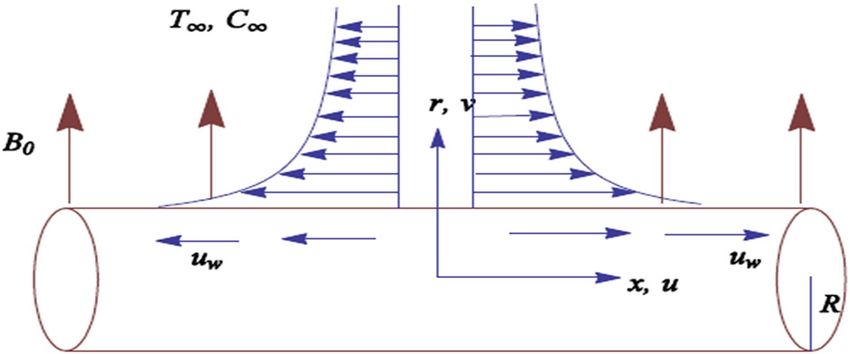
                                  Figure 2.  Plot of f for K .

                                  Numerical procedure
                                   For the nonlinear arrangement of equations and boundary conditions (9)–(13) the finite difference MATLAB
                                   bvp4c procedure is applied which is solid at 4th order and the grid size of 0.01 is viewed as acknowledged
                                  ­10–6. The numerical plan requires the change of higher-order differential equations into one-order differential
                                   equations.
                                                                              y1 = f , y2 = f ′ , y3 = f ′′ , yy1 = f ′′′ , y4 = θ, y5 = θ ′ , yy2 = θ ′′ ,
                                                                                                                                                                (23)
                                                                              y6 = φ, y7 = φ ′ , yy3 = φ ′′ , y8 = ξ , y9 = ξ ′ , yy4 = ξ ′′ ,
                                                                                                                                   
                                                                    −y1 y3 + y22 − 2My3 + β y1 y3 − 2y1 y3 + K 2 y2 + y1 + Fry2 y2
                                                                                                         
                                                          yy1 =                                                                     − ;
                                                                                              1 + 2Mη                                                           (24)
                                                               −2γ y5 − Pr y1 y5 − Pr (1 + 2Mη) Nb y5 y7 + Nt y52
                                                                                                                

                                                                                              2                             3   
                                                               − 43 Rd 3[θw − 1] 1 + [θw − 1]y4 (1 + 2Mη)y52 + 1 + y4 [θw − 1] My5
                                                                                                               
                                                         yy2 =                                               3                      ;                          (25)
                                                                             (1 + 2Mη) + 43 Rd 1 + [θw − 1]y4 (1 + 2Mη)
                                                                                              

                                                                                                                Nt
                                                                                                                      2My5 + (1 + 2Mηyy2 + ScMy6n
                                                                                                                                               
                                                                                      −2My7 − Scy1 y7 −         Nb
                                                                      yy3 =                                                                        ;            (26)
                                                                                                                     (1 + 2γ η)

                                                                                                                   (1 + 2Mη)y9 y6 + My8 y7 + σ My7
                                                                                                                                                      
                                                                                                      
                                                                              −2My9 − Lb Pr y1 y9            + Pe
                                                                                                                   σ (1 + 2Mη)y8 yy3 + (1 + 2Mη)y8 yy3          (27)
                                                           yy4 =                                                                                         ;
                                                                                                                  (1 + 2Mη)

                                                                y2 (0) − 1; y2 (0) − 1 − B1 y3 (0); y4 (0) − 1 − B2 y5 (0); y6 (0) − 1 − B3 y7 (0);
                                                                                                                                                                (28)
                                                                y8 (0) − 1 − B4 y9 (0); y2 (∞); y4 (∞); y6 (∞); y8 (∞);

                                  Results with discussion
                                 In this segment, we will examine the effect of distinct parameters on velocity, concentration, temperature, and
                                 gyrotactic microorganism fields. The numerous parameters like the magnetic interaction parameter (K), Darcy
                                 parameter (Fr), radiation parameter (Rd), Schmidt number (Sc), temperature ratio parameter (θw ), porosity
                                 parameter (), Deborah number (β), thermophoresis parameter (Nt), curvature parameter (M), bioconvection
                                 Lewis number (Lb), Prandtl number (Pr), Brownian motion parameter (Nb), wall roughness parameter (B1 ),
                                 chemical reaction parameter (γ ), concentration slip parameter (B3 ), thermal slip parameter (B3 ), Peclet number
                                 (Pe), Bioconvection parameter (σ ), and reaction order n are discussed on temperature, velocity and nanoparti-  ′
                                 cles concentration, and gyrotactic microorganism fields. Figure 2 demonstrated the behavior of K on the f (η).
                                 The strength of the Lorentz force is measured by K. The increase in K enhances the Lorentz force strength and
                                 due to the rise in K the velocity in axial direction decreases. As a result, the gradient of velocity at the surface

Scientific Reports |   (2021) 11:9391 |                              https://doi.org/10.1038/s41598-021-88947-5                                                    7

                                                                                                                                                              Vol.:(0123456789)
www.nature.com/scientificreports/

                                                     1

                                                   0.9

                                                   0.8

                                                   0.7

                                                   0.6

                                           f'( )
                                                   0.5

                                                   0.4                         B1 = 0, 0.05, 0.2, 0.5

                                                   0.3

                                                   0.2

                                                   0.1

                                                     0
                                                         0   0.5       1        1.5       2        2.5       3   3.5   4       4.5   5

                                                                           ′
                                            Figure 3.  Plot of f for B1.

                                                    1

                                                   0.9

                                                   0.8

                                                   0.7

                                                   0.6
                                           f'( )

                                                   0.5

                                                                           Fr = 0.0 , 0.4 , 0.8 , 1.2
                                                   0.4

                                                   0.3

                                                   0.2

                                                   0.1

                                                    0
                                                         0         1            2             3          4         5       6

                                                                           ′
                                            Figure 4.  Plot of f for Fr.

                                            is decreased. The wall B1 effect on the velocity profile is described in Fig. 3. The slip decreases the speed close
                                            to the disk and this condition enhances by increasing in K . Practically,    ′
                                                                                                                             the stretched impact of a cylinder is
                                            moderately
                                                   ′
                                                          shifted to the  liquid layers  which result in a decrease in f   (η). The influence of Fr on the velocity
                                            field f (η) is investigated in Fig. 4. It is examined that by escalating the variations of Fr , the decreasing trend of
                                            the velocity field is seen. This is because the higher values of Fr produce resistance in a liquid′ flow and hence
                                            velocity decreases. Figure 5 demonstrated the effect of the  on the velocity distribution of f (η). The liquid’s
                                            velocity diminishes on greater estimations of the . Actually, the movement of the liquid is stalled because of the
                                            presence
                                                   ′
                                                      of permeable media, and this results in the falloff of the liquid velocity. The effect of β on the velocity
                                            field f (η) is investigated in Fig. 6. It is examined that by escalating the variations of β , the diminishing behav-
                                            ior of the velocity field is seen. The impact of the θw upon θ (η) is explained by Fig. 7. A significant increase in
                                            θ(η) is observed. Enhancing θw signifies the temperature of the wall that causes thicker penetration depth for
                                            temperature profile. Likewise, the thermal diffusivity lies in the boundary layer with the relating exchange of
                                            heat. The thermal boundary layer corresponds to be larger nearby the region where the hotness is larger while it
                                            is lower a long way from cylinder because here temperature is low when compared to others. Subsequently, an
                                            intonation point emerges on the region when greater θw is considered. The temperature field for numerous M is
                                            shown in Fig. 8. A generous upgrade in the temperature of the liquid is seen when the radius of the cylinder is
                                            reduced. The effect of Pr on the thermal profile is described in Fig. 9. It is observed that the existence of melting
                                            phenomenon of the liquid temperature increases with rising variations of Pr. Therefore, we can judge that greater
                                            variation of Pr enhances the temperature field. Figure 10 defines that the large estimation of the B2 descends the
                                            dimensionless liquid’s temperature. From the figure, it is noticed that the thermal boundary layer becomes thicker

          Scientific Reports |   (2021) 11:9391 |                              https://doi.org/10.1038/s41598-021-88947-5                                        8

Vol:.(1234567890)
www.nature.com/scientificreports/

                                         0.9

                                         0.8

                                         0.7

                                         0.6

                                         0.5

                                 f'( )
                                         0.4
                                                                     = 0 , 0.15 , 0.30 , 0.45
                                         0.3

                                         0.2

                                         0.1

                                          0
                                               0       1               2            3           4       5         6

                                                                 ′
                                  Figure 5.  Plot of f for .

                                           1

                                         0.9

                                         0.8           = 0.0, 0.2, 0.4, 0.6
                                         0.7

                                         0.6
                                 f'( )

                                         0.5

                                         0.4

                                         0.3

                                         0.2

                                         0.1

                                           0
                                                   2       2.5             3             3.5        4       4.5       5

                                                                 ′
                                  Figure 6.  Plot of f for β.

                                  on enhancing the values of the curvature parameter. Figure 11 is outlined to show the plots of θ (η) for numerous
                                  terms of Rd when other variables are fixed. It can be judged that growing values of Rd increase the temperature
                                  and its parallel thickness of layer become thicker. Figure 12 elucidates that an increment in Sc decays the nano-
                                  particle concentration distribution φ(η). There is an opposite relationship between the Sc and the Brownian
                                  diffusion coefficient. Greater the values of Schmidt number Sc lower will be the Brownian diffusion coefficient,
                                  which tends to decrease the φ(η). Figure 13 portrays the concentration field for different estimations of γ . Large
                                  variations of the γ tend to smaller the nanoparticle concentration field. The descending behavior of a concentra-
                                  tion profile φ(η) on a B3 is drawn in Fig. 14. Figure 15 demonstrated that for greater values of reaction order n
                                  the concentration profile becomes higher. Figure 16 depicts the influence of Nt on φ(η). Both the concentration
                                  and thermal layer thickness are increased by accumulating the variations of the Nt . Greater estimations of the
                                  Nt give rise to thermophoresis force which increases the movement of nanoparticles from cold to hot surfaces
                                  and also increases in the thermal layer thickness. The descending behavior in concentration distribution φ(η)
                                  against Nb is shown in Fig. 17. An enhancement in Nb increases the Brownian motion due to which there is an
                                  escalation in the movement of nanoparticles and hence boundary layer thickness reduces. Figure 18 plotted to
                                  draw the curves of ξ (η) for different terms of Lb while other variables are fixed. It is observed that Lb depicts the
                                  decreasing behavior for large values of Lb. Figure 19 shows the behavior of Pe on gyrotactic microorganisms’

Scientific Reports |   (2021) 11:9391 |                              https://doi.org/10.1038/s41598-021-88947-5                                       9

                                                                                                                                                 Vol.:(0123456789)
www.nature.com/scientificreports/

                                                    1

                                                 0.9

                                                 0.8

                                                 0.7

                                                 0.6

                                           ( )   0.5

                                                                            w
                                                                                = 1.1 , 1.5 , 2 , 2.5
                                                 0.4

                                                 0.3

                                                 0.2

                                                 0.1

                                                    0
                                                        0   1       2       3         4       5         6       7       8   9   10

                                            Figure 7.  Plot of θ for θw.

                                                    1

                                                 0.9

                                                 0.8

                                                 0.7

                                                 0.6
                                           ( )

                                                 0.5

                                                 0.4                    M = 0 , 0.25 , 0.5 , 0.75

                                                 0.3

                                                 0.2

                                                 0.1

                                                    0
                                                        0       1       2            3            4         5       6       7        8

                                            Figure 8.  Plot of θ for M.

                                            profile ξ (η). Here, ξ (η) is an increasing function of Pe that effects to a decrease the diffusivity of microorgan-
                                            isms. Figure 20 indicates the variations in gyrotactic microorganism profile ξ (η) for distinct estimations of theσ .
                                            Large variations of σ decrease the gyrotactic microorganism field. Figure 21 is drawn to illustrates the impact of
                                            the Brinkman numbers on the Entropy generation number. It is found that Entropy escalates for the Brinkman
                                            number. In Fig. 22, with rising estimations of Re, an increase is seen in the entropy generation number. A higher
                                            Re causes more aggravation in the field and expand fluid friction and heat transfer, which eventually increases
                                            the rate of entropy in the boundary layer region.
                                               Table 2 is generated to substantiate the outlined results in this study by comparing it with Khan and ­Mustafa68
                                            and Tamoor et al.56 in limiting case. A good agreement between the two outcomes is seen. Besides, Tables 3, 4,
                                            5 express the numerical variations of the local Sherwood number Shx , local Nusselt number Nux , and density
                                            amount of motile microorganism Nnx for distinct estimations of K , M , θw , Rd , Pr , B1, B2, Sc , γ , k , Pe , Lb, and σ .

          Scientific Reports |   (2021) 11:9391 |                       https://doi.org/10.1038/s41598-021-88947-5                                                  10

Vol:.(1234567890)
www.nature.com/scientificreports/

                                          1

                                       0.9

                                       0.8

                                       0.7

                                       0.6

                                 ( )   0.5

                                       0.4

                                                          Pr = 7 , 8 , 9 ,10
                                       0.3

                                       0.2

                                       0.1

                                          0
                                              0   1   2          3       4         5   6   7   8   9      10

                                  Figure 9.  Plot of θ for Pr.

                                          1

                                       0.9

                                       0.8

                                       0.7

                                       0.6
                                 ( )

                                       0.5

                                       0.4
                                                           B2 = 0 , 0.5 , 1 ,1.5
                                       0.3

                                       0.2

                                       0.1

                                          0
                                              0   1   2          3        4        5   6   7   8   9      10

                                  Figure 10.  Plot of θ for B2.

                                  It is witnessed in Table 3 here that the heat flux rate is escalated for the growing estimates of K , but the opposite
                                  trend is perceived for the estimations of M , θw , Rd. In Table 4, it is witnessed that the mass flux rate is declined
                                  for the values of the Sc , and γ , however, it is enhanced for the increasing estimates of the M and n. The behavior of
                                  the varied parameters versus the density amount of motile microorganism is portrayed in Table 5. It is renowned
                                  that density amount of motile microorganism is improved for the estimations of M , Pr , σ , Pe , and Lb.

                                  Concluding remarks
                                  In the current investigation, we have discussed nonlinear radiative MHD Williamson nano liquid flow via a
                                  stretched cylinder in a Darcy–Forchheimer porous media. The flow is assisted by the impacts of the chemical
                                  reaction, and gyrotactic microorganisms with partial slip condition at the boundary. The solution to the problem

Scientific Reports |   (2021) 11:9391 |                      https://doi.org/10.1038/s41598-021-88947-5                                               11

                                                                                                                                                  Vol.:(0123456789)
www.nature.com/scientificreports/

                                                     1

                                                    0.9

                                                    0.8

                                                    0.7

                                                    0.6

                                                                                  Rd = 0.1 , 0.2 , 0.3 , 0.4

                                           ( )
                                                    0.5

                                                    0.4

                                                    0.3

                                                    0.2

                                                    0.1

                                                     0
                                                          0       1               2            3               4           5        6

                                            Figure 11.  Plot of θ for Rd.

                                                 0.8

                                                 0.7

                                                 0.6

                                                 0.5
                                           ( )

                                                 0.4

                                                 0.3
                                                                          Sc = 1 , 2 , 3 , 4

                                                 0.2

                                                 0.1

                                                    0
                                                        0     1       2       3       4        5      6            7   8       9   10

                                            Figure 12.  Plot of φ for Sc.

                                            is addressed by the MATLAB scheme of the bvp4c built-in function. The main results of the present investiga-
                                            tion are appended below:

                                            •    Nb and Nt show the opposing nature against the concentration field.
                                            •    The velocity distribution is lowered for large variations of K , Fr, and .
                                            •    Pe decreases the gyrotactic microorganism profile.
                                            •    An increment in Sc,B3, and γ leads to a lowering concentration profile.
                                            •    Enhanced variations of Pr and B2 display the decreasing behavior on the temperature profile.
                                            •    Large values of θw , Rd, and M causes an increment in temperature distribution.
                                            •    Gyrotactic microorganism profile reduces for greater variations of Lb and σ .
                                            •    Entropy intensifies for Br ; however, an opposite tendency is observed for β.

          Scientific Reports |   (2021) 11:9391 |                          https://doi.org/10.1038/s41598-021-88947-5                                12

Vol:.(1234567890)
www.nature.com/scientificreports/

                                          0.7

                                          0.6

                                          0.5

                                 ( )
                                          0.4

                                          0.3                         =0,1,2,3

                                          0.2

                                          0.1

                                              0
                                                  0   0.5         1           1.5         2       2.5         3       3.5

                                  Figure 13.  Plot of φ for γ .

                                          1

                                       0.9

                                       0.8

                                       0.7

                                       0.6
                                 ( )

                                       0.5

                                       0.4

                                                            B3 = 0 , 0.05 , 0.2 , 0.5
                                       0.3

                                       0.2

                                       0.1

                                          0
                                              0       0.5             1             1.5       2         2.5       3

                                  Figure 14.  Behaviour of φ for B3.

Scientific Reports |   (2021) 11:9391 |                        https://doi.org/10.1038/s41598-021-88947-5                       13

                                                                                                                            Vol.:(0123456789)
www.nature.com/scientificreports/

                                                    1

                                                 0.9

                                                 0.8

                                                 0.7

                                                 0.6

                                           ( )
                                                 0.5

                                                 0.4
                                                                  n = 1 , 1.5 , 2 , 3
                                                 0.3

                                                 0.2

                                                 0.1

                                                    0
                                                        0   0.5       1           1.5            2           2.5       3

                                            Figure 15.  Plot of φ for n.

                                                    1

                                                 0.9

                                                 0.8

                                                 0.7

                                                 0.6

                                                                             Nt = 0.1 , 0.2 ,0.3 , 0.4
                                           ( )

                                                 0.5

                                                 0.4

                                                 0.3

                                                 0.2

                                                 0.1

                                                    0
                                                        0   1        2           3           4           5         6       7

                                            Figure 16.  Plot of φ for Nt.

          Scientific Reports |   (2021) 11:9391 |                  https://doi.org/10.1038/s41598-021-88947-5                  14

Vol:.(1234567890)
www.nature.com/scientificreports/

                                          0.8

                                          0.7

                                          0.6

                                          0.5

                                 ( )
                                          0.4
                                                                         Nb = 0.1 , 0.2 , 0.3 , 0.4

                                          0.3

                                          0.2

                                          0.1

                                           0
                                                0       1        2          3         4           5       6       7        8

                                  Figure 17.  Plot of φ for Nb.

                                           1

                                          0.9

                                          0.8

                                          0.7

                                          0.6
                                 ( )

                                          0.5

                                          0.4

                                                                Lb = 0.5 , 0.6 , 0.7 , 0.8
                                          0.3

                                          0.2

                                          0.1

                                           0
                                                0   1       2        3          4     5       6       7       8       9   10

                                  Figure 18.  Plot of ξ for Lb.

Scientific Reports |   (2021) 11:9391 |                          https://doi.org/10.1038/s41598-021-88947-5                        15

                                                                                                                               Vol.:(0123456789)
www.nature.com/scientificreports/

                                                     1

                                                    0.9

                                                    0.8

                                                    0.7

                                                    0.6

                                           ( )      0.5

                                                    0.4

                                                                      Pe = 0.1 , 0.3 , 0.5 , 0.7
                                                    0.3

                                                    0.2

                                                    0.1

                                                     0
                                                          0   1   2       3       4        5    6   7   8   9      10

                                            Figure 19.  Plot of ξ for Pe.

                                                     1

                                                 0.9

                                                 0.8

                                                 0.7

                                                 0.6
                                           ( )

                                                 0.5

                                                 0.4

                                                                      = 0.2 , 0.4 , 0.6 , 0.8
                                                 0.3

                                                 0.2

                                                 0.1

                                                     0
                                                         0    1   2      3        4       5     6   7   8   9      10

                                            Figure 20.  Plot of ξ for σ.

          Scientific Reports |   (2021) 11:9391 |                     https://doi.org/10.1038/s41598-021-88947-5        16

Vol:.(1234567890)
www.nature.com/scientificreports/

                                          4

                                         3.5

                                          3

                                                                         Br = 0.1, 0.2, 0.3,
                                         2.5                             0.4, 0.5

                                 NG
                                          2

                                                           Br = 0.2 , 0.4 , 0.6 , 0.8
                                         1.5

                                          1

                                         0.5
                                               0      0.1       0.2      0.3        0.4        0.5     0.6   0.7       0.8   0.9         1

                                  Figure 21.  Plot of NG for Br.

                                          35

                                          30

                                          25

                                          20
                                 NG

                                          15

                                                                      Re = 0.1, 0.2, 0.3, 0.4, 0.5
                                          10

                                           5

                                           0
                                               0               0.5                 1                 1.5           2               2.5       3

                                  Figure 22.  Plot of NG for Re.

                                               −f ′′ (0)        −f ′′ (0)      −f ′′ (0)
                                   K           68               56
                                                                               Present
                                   0           1                1              1
                                   0.2         1.0198039        1.01980        1.01981
                                   0.5         1.1180340        1.11803        1.11803
                                   0.8         1.2806248        1.28063        1.28062
                                   1           1.4142136        1.41421        1.41421

                                  Table 2.  Validation of numerical outcomes for −f ′′ (0) with Khan and ­Mustafa68 and Tamoor et al.56 and when
                                  M = B1 = 0.

Scientific Reports |   (2021) 11:9391 |                                https://doi.org/10.1038/s41598-021-88947-5                                    17

                                                                                                                                                 Vol.:(0123456789)
www.nature.com/scientificreports/

                                                                                 1
                                             K      M     θw    Rd      (Rex )− 2 Nux
                                             0.5    0.2   1.5           0.7654
                                             1                          0.6803
                                             1.5                        0.5851
                                             2                          0.5003
                                                    0.5                 0.7745
                                                    0.7                 0.7801
                                                    1                   0.7883
                                                          2             1.1440
                                                          2.5           1.4871
                                                          3             1.7770
                                                                0.1     1.3736
                                                                0.3     2.2339
                                                                0.5     3.3713

                                                                                     1
                                            Table 3.  Computations of (Rex ) 2 Nux for various variations of K , M , θw , Rd when Pr = 7 and B1 = B2 = 0.5.

                                                                                 1
                                             M      Sc    γ     n       (Rex )− 2 Shx
                                             0.2    5     1     1       1.15817
                                             0.5                        1.17480
                                             0.7                        1.18683
                                             1                          1.20568
                                                    2                   0.97565
                                                    3                   1.05478
                                                    7                   1.22726
                                                          2             1.27036
                                                          3             1.34142
                                                          4             1.39264
                                                                2       0.99641
                                                                3       0.92496
                                                                5       0.87854

                                                                                         1
                                            Table 4.  Computations of (Rex )− 2 Shx for numerous variations of Sc,M , and γ when Pr = 7, k = 0.5 and
                                            B1 = B2 = B3 = 0.5.

                                                                                             1
                                             M      Pr    σ     Pe      Lb       (Rex )− 2 Nnx
                                             0.3    1.5   0.2   0.3     0.2      0.935596
                                             0.6                                 1.059580
                                             0.9                                 1.193600
                                                    1.0                          0.915801
                                                    1.5                          0.935596
                                                    2.0                          0.940771
                                                          0.2                    0.935596
                                                          0.4                    1.012580
                                                          0.6                    1.089560
                                                                0.4              1.065290
                                                                0.5              1.189010
                                                                0.6              1.307130
                                                                        0.3      0.963155
                                                                        0.6      1.038210
                                                                        0.9      1.103780

                                                                                         1
                                            Table 5.  Computations of (Rex )− 2 Nnx for various variations of M , Pr , σ , Pe and Lb.

          Scientific Reports |   (2021) 11:9391 |                   https://doi.org/10.1038/s41598-021-88947-5                                                18

Vol:.(1234567890)
www.nature.com/scientificreports/

                                  Received: 21 January 2021; Accepted: 19 April 2021

                                  References
                                   1. Choi, S. U. S., & Eastman, J. A. Enhancing thermal conductivity of fluids with nanoparticles. (IMECE). 66, 99–105 (1995).
                                   2. Koo, J. & Kleinstreuer, C. Laminar nanofluid flow in microheat-sinks. Int. J. Heat Mass Transf. 48(13), 2652–2661 (2005).
                                   3. Eastman, J. A., Choi, S. U. S., Li, S., Yu, W. & Thompson, L. J. Anomalously increased effective thermal conductivities of ethylene
                                      glycol-based nanofluids containing copper nanoparticles. Appl. Phys. Lett. 78(6), 718–720 (2001).
                                   4. Choi, S. U. S., Zhang, Z. G., Yu, W., Lockwood, F. E. & Grulke, E. A. Anomalous thermal conductivity enhancement in nanotube
                                      suspensions. Appl. Phys. Lett. 79(14), 2252–2254 (2001).
                                   5. Bilal, M., Mazhar, S. Z., Ramzan, M. & Mehmood, Y. Time-dependent hydromagnetic stagnation point flow of a Maxwell nanofluid
                                      with melting heat effect and amended Fourier and Fick’s laws. Heat Trans. https://​doi.​org/​10.​1002/​htj.​22081 (2021).
                                   6. Tlili, I., Naseer, S., Ramzan, M., Kadry, S. & Nam, Y. Effects of chemical species and nonlinear thermal radiation with 3D Maxwell
                                      nanofluid flow with double stratification—an analytical solution. Entropy 22(4), 453 (2020).
                                   7. Sheikholeslami, M., Arabkoohsar, A., & Jafaryar, M. (2020). Impact of a helical-twisting device on the thermal--hydraulic perfor-
                                      mance of a nanofluid flow through a tube. J. Therm. Anal. Calorim. 139(5), 3317–3329 (2020).
                                   8. Farooq, U. et al. MHD flow of Maxwell fluid with nanomaterials due to an exponentially stretching surface. Sci. Rep. 9(1), 1–11
                                      (2019).
                                   9. Ramesh, G. K., Shehzad, S. A., Rauf, A. & Chamkha, A. J. Heat transport analysis of aluminum alloy and magnetite graphene oxide
                                      through permeable cylinder with heat source/sink. Phys. Scr. 95(9), 095203 (2020).
                                  10. Reza-E-Rabbi, S., Ahmmed, S. F., Arifuzzaman, S. M., Sarkar, T. & Khan, M. S. Computational modelling of multiphase fluid flow
                                      behaviour over a stretching sheet in the presence of nanoparticles. Int. J. Eng. Sci. Technol. 23(3), 605–617 (2020).
                                  11. Abbasi, A., Mabood, F., Farooq, W. & Hussain, Z. Non-orthogonal stagnation point flow of Maxwell nano-material over a stretching
                                      cylinder. Int. Comm. Heat Mass. Tran. 120, 105043 (2021).
                                  12. Li, F. et al. Numerical study for nanofluid behavior inside a storage finned enclosure involving melting process. J. Mol. Liq. 297,
                                      111939 (2020).
                                  13. Komeilibirjandi, A., Raffiee, A. H., Maleki, A., Nazari, M. A. & Shadloo, M. S. Thermal conductivity prediction of nanofluids con-
                                      taining CuO nanoparticles by using correlation and artificial neural network. J. Therm. Anal. Calorim. 139(4), 2679–2689 (2020).
                                  14. Waqas, H., Imran, M. & Bhatti, M. M. Influence of bioconvection on Maxwell nanofluid flow with the swimming of motile micro-
                                      organisms over a vertical rotating cylinder. Chin. J. Phys. 68, 558–577 (2020).
                                  15. Islam, S., Khan, A., Kumam, P., Alrabaiah, H., Shah, Z., Khan, W., & Jawad, M. Radiative mixed convection flow of Maxwell
                                      nanofluid over a stretching cylinder with Joule heating and heat source/sink effects. Sci. Rep. 10(1), 1–18 (2020).
                                  16. Ahmed, A., Khan, M. & Ahmed, J. Thermal analysis in swirl motion of Maxwell nanofluid over a rotating circular cylinder. Appl.
                                      Math. Mech. 41(9), 1417–1430 (2020).
                                  17. Kumar, R. V., Gowda, R. P., Kumar, R. N., Radhika, M. & Prasannakumara, B. C. Two-phase flow of dusty fluid with suspended
                                      hybrid nanoparticles over a stretching cylinder with modified Fourier heat flux. Appl. Sci. 3(3), 1–9 (2021).
                                  18. Kumar, R. N., Gowda, R. P., Abusorrah, A. M., Mahrous, Y. M., Abu-Hamdeh, N. H., Issakhov, A., & Prasannakumara, B. C. Impact
                                      of magnetic dipole on ferromagnetic hybrid nanofluid flow over a stretching cylinder. Phys. Scr. 96(4), 045215 (2021).
                                  19. Jayadevamurthy, P. G. R., Rangaswamy, N. K., Prasannakumara, B. C., & Nisar, K. S. Emphasis on unsteady dynamics of bioconvec-
                                      tive hybrid nanofluid flow over an upward–downward moving rotating disk. Num. Methods Part. Diff. Equ. (2020).
                                  20. Khan, S. U., Shehzad, S. A., & Ali, N. Bioconvection flow of magnetized Williamson nanoliquid with motile organisms and variable
                                      thermal conductivity. Appl. Nanosci. 1–12 (2020).
                                  21. Ramesh, G. K., Gireesha, B. J. & Gorla, R. S. R. Study on Sakiadis and Blasius flows of Williamson fluid with convective boundary
                                      condition. Nonlinear Eng. 4(4), 215–221 (2015).
                                  22. Anwar, M. I., Rafique, K., Misiran, M., Shehzad, S. A., & Ramesh, G. K. Keller-box analysis of inclination flow of magnetized Wil-
                                      liamson nanofluid. Appl. Sci. 2(3), 1–9 (2020).
                                  23. Darcy, H. Les fontaines publiques de la ville de Dijon: exposition et application...Victor Dalmont (1856).
                                  24. Forchheimer, P. Wasserbewegung durch boden. Z. Ver. Deutsch, Ing., 45, 1782–1788 (1901).
                                  25. Muskat, M. The flow of homogeneous fluids through porous media (No. 532.5 M88) (1946).
                                  26. Pal, D. & Mondal, H. Hydromagnetic convective diffusion of species in Darcy–Forchheimer porous medium with non-uniform
                                      heat source/sink and variable viscosity. Int. Commun. Heat Mass Transf. 39(7), 913–917 (2012).
                                  27. Ganesh, N. V., Hakeem, A. A. & Ganga, B. Darcy–Forchheimer flow of hydromagneticnanofluid over a stretching/shrinking sheet
                                      in a thermally stratified porous medium with second order slip, viscous and Ohmic dissipations effects. Ain Shams Eng. J. 9(4),
                                      939–951 (2016).
                                  28. Alshomrani, A. S. & Ullah, M. Z. Effects of homogeneous-heterogeneous reactions and convective condition in Darcy–Forchheimer
                                      flow of carbon nanotubes. J. Heat Transfer. 141(1), 012405 (2019).
                                  29. Saif, R. S., Hayat, T., Ellahi, R., Muhammad, T., & Alsaedi, A. Darcy–Forchheimerflow of nanofluid due to a curved stretching
                                      surface. Int. J. Num. Method H. 29, (2018).
                                  30. Seth, G. S., Kumar, R. & Bhattacharyya, A. Entropy generation of dissipative flow of carbon nanotubes in rotating frame with
                                      Darcy–Forchheimer porous medium: A numerical study. J. Mol. Liq. 268, 637–646 (2018).
                                  31. Hayat, T., Ra…que, K., Muhammad, T., Alsaedi, A., & Ayub, M. Carbon nanotubessignificance in Darcy–Forchheimer flow. Res.
                                      Phys. 8, 26–33 (2018).
                                  32. Ramesh, G. K., Kumar, K. G., Gireesha, B. J., Shehzad, S. A. & Abbasi, F. M. Magnetohydrodynamic nanoliquid due to unsteady
                                      contracting cylinder with uniform heat generation/absorption and convective condition. Alex. Eng. J. 57(4), 3333–3340 (2018).
                                  33. Arifuzzaman, S. M. et al. Hydrodynamic stability and heat and mass transfer flow analysis of MHD radiative fourth-grade fluid
                                      through porous plate with chemical reaction. King Saud Univ. Sci. 31(4), 1388–1398 (2019).
                                  34. Reza-E-Rabbi, S., Arifuzzaman, S. M., Sarkar, T., Khan, M. S. & Ahmmed, S. F. Explicit finite difference analysis of an unsteady
                                      MHD flow of a chemically reacting Casson fluid past a stretching sheet with Brownian motion and thermophoresis effects. J. King
                                      Saud Univ. Sci. 32(1), 690–701 (2020).
                                  35. Arifuzzaman, S. M., Khan, M. S., Mehedi, M. F. U., Rana, B. M. J. & Ahmmed, S. F. Chemically reactive and naturally convective
                                      high speed MHD fluid flow through an oscillatory vertical porous plate with heat and radiation absorption effect. Eng. Sci. Technol.
                                      21(2), 215–228 (2018).
                                  36. Shankaralingappa, B. M., Gireesha, B. J., Prasannakumara, B. C., & Nagaraja, B. Darcy–Forchheimer flow of dusty tangent hyper-
                                      bolic fluid over a stretching sheet with Cattaneo-Christov heat flux. Waves Rand. Comp. Media. 1–20 (2021).
                                  37. Ramzan, M., Abid, N., Lu, D. & Tlili, I. Impact of melting heat transfer in the time-dependent squeezing nanofluid flow contain-
                                      ing carbon nanotubes in a Darcy–Forchheimer porous media with Cattaneo-Christov heat flux. Comm. Theo. Phy. 72(8), 085801
                                      (2020).
                                  38. Jawad, M., Saeed, A., Kumam, P., Shah, Z. & Khan, A. Analysis of boundary layer MHD Darcy–Forchheimer radiative nanofluid
                                      flow with Soret and Dufour effects by means of marangoni convection. Case Stud. 23, 100792 (2021).

Scientific Reports |   (2021) 11:9391 |                   https://doi.org/10.1038/s41598-021-88947-5                                                                   19

                                                                                                                                                                  Vol.:(0123456789)
www.nature.com/scientificreports/

                                            39. Khan, M. I. Transportation of hybrid nanoparticles in forced convective Darcy–Forchheimer flow by a rotating disk. Int Com. Heat
                                                Mass Tran. 122, 105177 (2021).
                                            40. Muhammad, T. et al. Significance of Darcy–Forchheimer porous medium in nanofluid through carbon nanotubes. Comm. Theo.
                                                Phys. 70(3), 361 (2018).
                                            41. Ramzan, M., Gul, H., & Zahri, M. Darcy–Forchheimer 3D Williamson nanofluid flow with generalized Fourier and Fick’s laws in
                                                a stratified medium. Bull. Polish Acad. Sci. Tech. Sci. 68(2) (2020).
                                            42. Mehmood, T., Ramzan, M., Howari, F., Kadry, S. & Chu, Y. M. Application of response surface methodology on the nanofluid flow
                                                over a rotating disk with autocatalytic chemical reaction and entropy generation optimization. Sci. Rep. 11(1), 1–18 (2021).
                                            43. Ramzan, M., Chung, J. D., Kadry, S., Chu, Y. M. & Akhtar, M. Nanofluid flow containing carbon nanotubes with quartic autocata-
                                                lytic chemical reaction and Thompson and Troian slip at the boundary. Sci. Rep. 10(1), 1–13 (2020).
                                            44. Khan, M. et al. 3-D axisymmetric Carreau nanofluid flow near the Homann stagnation region along with chemical reaction:
                                                Application Fourier’s and Fick’s laws. Math. Comp. Sim. 170, 221–235 (2020).
                                            45. Lu, D. C., Ramzan, M., Bilal, M., Chung, J. D. & Farooq, U. A numerical investigation of 3D MHD rotating flow with binary chemi-
                                                cal reaction, activation energy and non-Fourier heat flux. Comm. Theo. Phys. 70(1), 089 (2019).
                                            46. Khan, M., Malik, M. Y., Salahuddin, T. & Khan, F. Generalized diffusion effects on Maxwell nanofluid stagnation point flow over
                                                a stretchable sheet with slip conditions and chemical reaction. J. Braz. Soc. Mech. Sci. Eng. 41(3), 1–9 (2019).
                                            47. Ramzan, M., Bilal, M. & Chung, J. D. Numerical simulation of magnetohydrodynamic radiative flow of Casson nanofluid with
                                                chemical reaction past a porous media. Theo. Nanosci. 14(12), 5788–5796 (2017).
                                            48. Khan, M., Shahid, A., Malik, M. Y. & Salahuddin, T. Chemical reaction for Carreau-Yasuda nanofluid flow past a nonlinear stretch-
                                                ing sheet considering Joule heating. Res. Phys 8, 1124–1130 (2018).
                                            49. Khan, M. et al. 3-D axisymmetric Carreau nanofluid flow near the Homann stagnation region along with chemical reaction:
                                                application Fourier’s and Fick’s laws. Math. Compt. Simul. 170, 221–235 (2020).
                                            50. Rehman, K. U., Khan, A. A., Malik, M. Y. & Pradhan, R. K. Combined effects of Joule heating and chemical reaction on non-
                                                Newtonian fluid in double stratified medium: A numerical study. Res. Phys. 7, 3487–3496 (2017).
                                            51. Ramzan, M., Gul, H. & Chung, J. D. Double stratified radiative Jeffery magneto nanofluid flow along an inclined stretched cylinder
                                                with chemical reaction and slip condition. Eur. Phys. J. Plus 132(11), 1–17 (2017).
                                            52. Lu, D., Ramzan, M., Ahmad, S., Chung, J. D. & Farooq, U. Upshot of binary chemical reaction and activation energy on carbon
                                                nanotubes with Cattaneo-Christov heat flux and buoyancy effects. Phys. Fluids. 29(12), 123103 (2017).
                                            53. Sohail, M., Naz, R. & Abdelsalam, S. I. On the onset of entropy generation for a nanofluid with thermal radiation and gyrotactic
                                                microorganisms through 3D flows. Phys. Scr. 95(4), 045206 (2020).
                                            54. Khan, M. I., Qayyum, S., Hayat, T., Khan, M. I. & Alsaedi, A. Entropy optimization in flow of Williamson nanofluid in the presence
                                                of chemical reaction and Joule heating. Int. J. Heat Mass Transf. 133, 959–967 (2019).
                                            55. Sarojamma, G., Vijaya Lakshmi, R., Satya Narayana, P. V. & Animasaun, I. L. Exploration of the significance of autocatalytic chemi-
                                                cal reaction and Cattaneo-Christov heat flux on the dynamics of a micropolar fluid. J. Appl. Comput. Mech. 6(1), 77–89 (2020).
                                            56. Tamoor, M., Waqas, M., Khan, M. I., Alsaedi, A. & Hayat, T. Magnetohydrodynamic flow of Casson fluid over a stretching cylinder.
                                                Res. Phys. 7, 498–502 (2017).
                                            57. Yusuf, T. A. & Gbadeyan, J. A. Entropy generation on Maxwell fluid flow past an inclined stretching plate with slip and convective
                                                surface conditon: Darcy–Forchheimer model. NHC. 26, 62–83 (2019).
                                            58. Adesanya, S. O., Dairo, O. F., Yusuf, T. A., Onanaye, A. S., & Arekete, S. A. Thermodynamics analysis for a heated gravity-driven
                                                hydromagnetic couple stress film with viscous dissipation effects. Phys. A. 540, 123150 (2020).
                                            59. Yusuf, T. A., Adesanya, S. O. & Gbadeyan, J. A. Entropy generation in MHD Williamson nanofluid over a convectively heated
                                                stretching plate with chemical reaction. J. Heat Transfer. 49(4), 1982–1999 (2020).
                                            60. Mabood, F., Yusuf, T. A., & Sarris, I. E. Entropy generation and irreversibility analysis on free convective unsteady MHD Casson
                                                fluid flow over a stretching sheet with Soret/Dufour in porous media. Int. J. 11(6), (2020).
                                            61. Mabood, F., Yusuf, T. A., & Khan, W. A. (2021). Cu–Al2 ­O3–H2O hybrid nanofluid flow with melting heat transfer, irreversibility
                                                analysis and nonlinear thermal radiation. J. Therm. Anal. Calorim. 143(2), 973–984 (2021).
                                            62. Mabood, F., Yusuf, T. A., & Bognár, G. Features of entropy optimization on MHD couple stress nanofluid slip flow with melting
                                                heat transfer and nonlinear thermal radiation. Sci. Rep. 10(1), 1–13 (2020).
                                            63. Mabood, F., Yusuf, T. A., Rashad, A. M., Khan, W. A. & Nabwey, H. A. Effects of combined heat and mass transfer on entropy
                                                generation due to MHD nanofluid flow over a rotating frame. CMC. 66(1), 575–587 (2021).
                                            64. Yusuf, T. A., Mabood, F., Khan, W. A. & Gbadeyan, J. A. Irreversibility analysis of Cu-TiO2-H2O hybrid-nanofluid impinging on
                                                a 3-D stretching sheet in a porous medium with nonlinear radiation: Darcy–Forchhiemer’s model. Alex. Eng. J. 59, 5247–5261
                                                (2020).
                                            65. Almeida, F., Gireesha, B. J., Venkatesh, P., & Ramesh, G. K. Intrinsic irreversibility of ­Al2O3–H2O nanofluid Poiseuille flow with
                                                variable viscosity and convective cooling. Int. J. Numer. Method H. (2020).
                                            66. Hayat, T., Rashid, M., Alsaedi, A. & Asghar, S. Nonlinear convective flow of Maxwell nanofluid past a stretching cylinder with
                                                thermal radiation and chemical reaction. J. Braz. Soc. Mech. Sci. Eng. 41(2), 86 (2019).
                                            67. Raju, C. S. K. et al. The flow of magnetohydrodynamic Maxwell nanofluid over a cylinder with Cattaneo-Christov heat flux model.
                                                Cont. Mech. Thermodyn. 29(6), 1347–1363 (2017).
                                            68. Khan, J. A. & Mustafa, M. A numerical analysis for non-linear radiation in MHD flow around a cylindrical surface with chemically
                                                reactive species. Res. Phys. 8, 963–970 (2018).

                                            Acknowledgements
                                            The authors extend their appreciation to the Deanship of Scientific Research at King Khalid University, Abha
                                            61413, Saudi Arabia for funding this work through research groups program under Grant number RGP-1-96-42.

                                            Author contributions
                                            M.R. did conceptualization, M.U.K. worked on methodology, C.L. did validation and formal analysis, Y.M.C.
                                            wrote the original draft, S.K., and C.L. worked on software. Y.M.C. arranged the funds, M.Y.M and R.C. helped
                                            in the revised draft and partial funding arrangements.

                                            Funding
                                            The research was supported by the National Natural Science Foundation of China (Grant Nos. 11971142,
                                            11871202, 61673169, 11701176, 11626101, 11601485).

                                            Competing interests
                                            The authors declare no competing interests.

          Scientific Reports |   (2021) 11:9391 |                   https://doi.org/10.1038/s41598-021-88947-5                                                                  20

Vol:.(1234567890)
www.nature.com/scientificreports/

                                  Additional information
                                  Correspondence and requests for materials should be addressed to Y.-M.C.
                                  Reprints and permissions information is available at www.nature.com/reprints.
                                  Publisher’s note Springer Nature remains neutral with regard to jurisdictional claims in published maps and
                                  institutional affiliations.
                                                Open Access This article is licensed under a Creative Commons Attribution 4.0 International
                                                License, which permits use, sharing, adaptation, distribution and reproduction in any medium or
                                  format, as long as you give appropriate credit to the original author(s) and the source, provide a link to the
                                  Creative Commons licence, and indicate if changes were made. The images or other third party material in this
                                  article are included in the article’s Creative Commons licence, unless indicated otherwise in a credit line to the
                                  material. If material is not included in the article’s Creative Commons licence and your intended use is not
                                  permitted by statutory regulation or exceeds the permitted use, you will need to obtain permission directly from
                                  the copyright holder. To view a copy of this licence, visit http://​creat​iveco​mmons.​org/​licen​ses/​by/4.​0/.

                                  © The Author(s) 2021

Scientific Reports |   (2021) 11:9391 |                https://doi.org/10.1038/s41598-021-88947-5                                                21

                                                                                                                                             Vol.:(0123456789)
You can also read