A California Statewide Three-Dimensional Seismic Velocity Model from Both Absolute and Differential Times
←
→
Page content transcription
If your browser does not render page correctly, please read the page content below
Bulletin of the Seismological Society of America, Vol. 100, No. 1, pp. 225–240, February 2010, doi: 10.1785/0120090028

                                                                                                                                             Ⓔ

               A California Statewide Three-Dimensional Seismic Velocity
                   Model from Both Absolute and Differential Times
          by Guoqing Lin,* Clifford H. Thurber, Haijiang Zhang,† Egill Hauksson, Peter M. Shearer,
                     Felix Waldhauser, Thomas M. Brocher, and Jeanne Hardebeck

                  Abstract       We obtain a seismic velocity model of the California crust and uppermost
                  mantle using a regional-scale double-difference tomography algorithm. We begin
                  by using absolute arrival-time picks to solve for a coarse three-dimensional (3D) P ve-
                  locity (V P ) model with a uniform 30 km horizontal node spacing, which we then use as
                  the starting model for a finer-scale inversion using double-difference tomography
                  applied to absolute and differential pick times. For computational reasons, we split
                  the state into 5 subregions with a grid spacing of 10 to 20 km and assemble our final
                  statewide V P model by stitching together these local models. We also solve for a state-
                  wide S-wave model using S picks from both the Southern California Seismic Network
                  and USArray, assuming a starting model based on the V P results and a V P =V S ratio of
                  1.732. Our new model has improved areal coverage compared with previous models,
                  extending 570 km in the SW–NE direction and 1320 km in the NW–SE direction. It also
                  extends to greater depth due to the inclusion of substantial data at large epicentral
                  distances. Our V P model generally agrees with previous separate regional models
                  for northern and southern California, but we also observe some new features, such
                  as high-velocity anomalies at shallow depths in the Klamath Mountains and Mount
                  Shasta area, somewhat slow velocities in the northern Coast Ranges, and slow anoma-
                  lies beneath the Sierra Nevada at midcrustal and greater depths. This model can be
                  applied to a variety of regional-scale studies in California, such as developing a unified
                  statewide earthquake location catalog and performing regional waveform modeling.

                     Online Material: Smoothing and damping trade-off analysis, a priori Moho depth,
                  resolution tests, and map-view slices and cross sections through the 3D V P and V S
                  models.

                           Introduction
     Numerous studies of velocity structure in California have                  model for locating earthquakes in California. In this study,
been done with varying scales in different areas (Table 1).                     we take advantage of the regional-scale double-difference
The largest and most complete crustal tomography models                         (DD) tomography algorithm (Zhang and Thurber, 2006) to
in California are the recent southern California model by                       develop P- and S-wave velocity models for the entire state
Lin et al. (2007) and the northern California model by Thurber                  of California. Our P velocity model is derived from both
et al. (2009). These studies have revealed key features of the                  first-arrival absolute and differential time picks obtained from
crustal structure of California. The integration of the Northern                the California seismic networks and has a horizontal grid
and Southern California Seismic Networks (NCSN and SCSN)                        spacing as fine as 10 km. The S velocity model is solved using
into a unified statewide network, the California Integrated                     the SCSN and USArray picks with a horizontal grid spacing
Seismic Network (CISN; e.g., Hellweg et al., 2007), has                         of 30 km. There are numerous tomographic studies in
motivated the development of a statewide seismic velocity                       California and it is impractical to compare our model with
                                                                                all of them; we focus on a comparison with the recent
   *Now at Division of Marine Geology and Geophysics, Rosenstiel School         regional-scale tomographic studies for southern and northern
of Marine and Atmospheric Science, University of Miami, Miami, Florida,         California by Lin et al. (2007) and Thurber et al. (2009).
33149 (glin@rsmas.miami.edu).
   †
                                                                                Because our V P and V S models are solved using different sets
     Also at Department of Geoscience, University of Wisconsin–Madison,
1215 W. Dayton St., Madison, Wisconsin 53706.                                   of data and the V P model has better resolution, we present

                                                                          225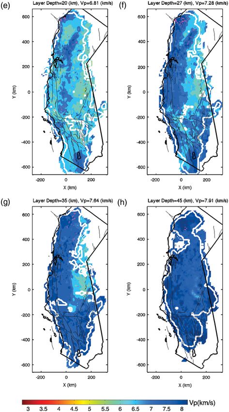
226 G. Lin, C. H. Thurber, H. Zhang, E. Hauksson, P. M. Shearer, F. Waldhauser, T. M. Brocher, and J. Hardebeck
42˚
Kl Mou
Mount Shasta Volcanic Plateau
am n
A
at tain
h
Lake Shasta
Lake Almanor
s
Mendocino
Fracture
Zone
Ma
40˚ Lake Basin
Oroville B’
aca ast R
Lake and
Co
ma
Tahoe
Range
Fau nges
Sie
Province
lt
a
rra
HRC
Ne
GV
va
d
38˚ San C’
a
Francisco
Gr Coa
W
hi
te
ea
SFB
SA
M
t V Ran
ou
F
Owens
nt
all
ai
st
ns
ey
Sier
B
Valle y
ge
ra Nevada
Death
Sa
s
N
36˚
lin
Parkfield Valley
ev lifo
Coso
ia
ad rn
Cholame
C
n
a
SSJV
a ia
Bl
oc
GF
Pa
k
SA
c
F
ific
Mojave Desert
C TR SA
-O
F
ce
VB SG Landers
Northridge M
an
SMM WN SBM
34˚ Los
Angeles
California Pe
n ins
Continental
SJ E
ula
Borderland
rR
IM
an
San
ge
Diego
s
Baja California
32˚ 200 km
A’
-126˚ -124˚ -122˚ -120˚ -118˚ -116˚ -114˚
Figure 1. Map of selected geological and geographic features in our study area. The thick straight lines indicate the model cross sections
shown in Figure 7. The NW–SE profile A-A’ is parallel to the San Andreas fault, and the SW–NE profiles B-B’ and C-C’ are perpendicular to
the San Andreas fault. Abbreviations: E, Elsinore fault; GF, Garlock fault; GV, Green Valley fault; HRC, Healdsburg–Rodgers Creek
fault; IM, Imperial Valley fault; SAF, San Andreas fault; SBM, San Bernardino Mountains; SFB, San Francisco Bay; SGM, San Gabriel
Mountains; SJ, San Jacinto fault; SMM, Santa Monica Mountains; SSJV, Southern San Joaquin Valley; TR, Transverse Ranges; VB, Ventura
basin; WN, Whittier Narrows.
them separately with more emphasis on the V P model. 3668 events from the Southern California Seismic Network,
Figure 1 shows selected geological and geographic features and 727 events from the Pacific Gas and Electric seismic
in our study and the positions of three profiles for the velocity network (blue, pink, and green dots in Fig. 2a, respectively).
cross sections. These earthquakes were selected based on having the great-
est number of P picks among those events within a 6 km
P-Wave Velocity Model radius, with a magnitude threshold of 2.5. The total number
of P picks in our data set is 551,318 with an average of 63
Data and Inversion Method picks per event. In order to improve constraints on the shal-
The data sets for our V P model are the first-arrival low crustal structure, we assembled first-arrival times from
absolute and differential times of 8720 earthquakes recorded 3110 explosions and airguns (red circles in Fig. 2b) recorded
by the seismic networks in California, consisting of 4325 on profile receivers and network stations. The principal
events from the Northern California Seismic Network, active-source data sets and sources are listed in Table 2.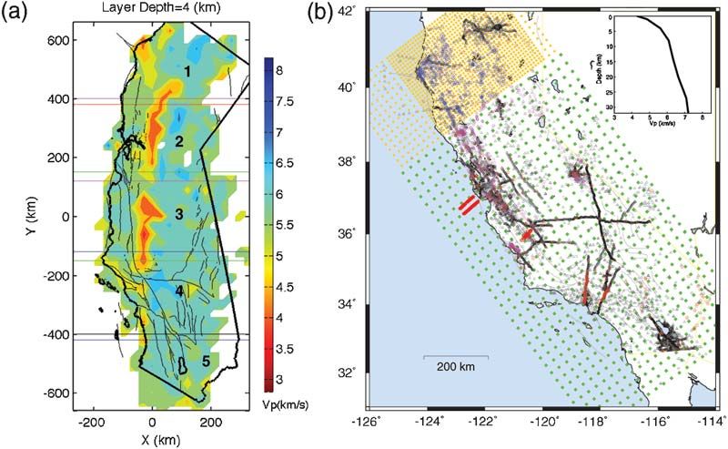
A California Statewide Three-Dimensional Seismic Velocity Model 227
(a) (b)
earthquake from NCSN shot
42˚ earthquake from PG&E 42˚ quarry blast
earthquake from SCSN
40˚ 40˚
38˚ 38˚
36˚ 36˚
34˚ 34˚
32˚ 32˚
200 km 200 km
30˚ 30˚
-126˚ -124˚ -122˚ -120˚ -118˚ -116˚ -114˚ -126˚ -124˚ -122˚ -120˚ -118˚ -116˚ -114˚
(c) (d) 0
5 grid node
42˚ 42˚ x
Depth (km)
10
15
20
25
40˚ 40˚
30
0 3 4 5 6 7 8
60
y= Vp (km/s)
0
38˚ 38˚ 45
y=
0
30
y=
36˚ 36˚ 15
0
y=
Y 0
y=
34˚ 34˚ 50
-1
y=
x=
00
27
-3
x=
y=
0
18
32˚ 32˚ x=
0
50 90
-4
x=
200 km 200 km y=
0
x=
-9
00
0
x=
-6
-1
y=
30˚ 30˚
80
-126˚ -124˚ -122˚ -120˚ -118˚ -116˚ -114˚ -126˚ -124˚ -122˚ -120˚ -118˚ -116˚ -114˚
Figure 2. Event and station distributions in our study area and starting inversion grid nodes for the 3D coarse model (30-km horizontal
spacing). (a) earthquakes; (b) controlled sources; (c) stations; (d) inversion grid nodes (small panel shows the 1D starting velocity model).
Quarry blasts, which have known locations but unknown ori- and Thurber, 2006), which is a generalization of DD location
gin times, are also valuable to be included in tomographic (Waldhauser and Ellsworth, 2000). It maps a spherical-
inversions because they provide constraints that are almost Earth coordinate system into a Cartesian coordinate system
as good as the active-source data. We include data from (a sphere in a box; Flanagan et al., 2007) and incorporates a
44 quarry blasts (blue circles in Fig. 2b), with 19 in south- finite-difference travel time calculator and spatial smoothing
ern California (see Lin et al., 2007) and 25 in northern constraints. This algorithm is designed to solve jointly for 3D
California. Figure 2c shows the locations of temporary and velocity structure and earthquake locations using both first-
network stations used in our study. arrival times and differential times, leading to improved res-
The model presented in this study is obtained by using a olution in the seismically active areas where the differential
regional-scale DD tomography algorithm (tomoFDD; Zhang data provide dense sampling.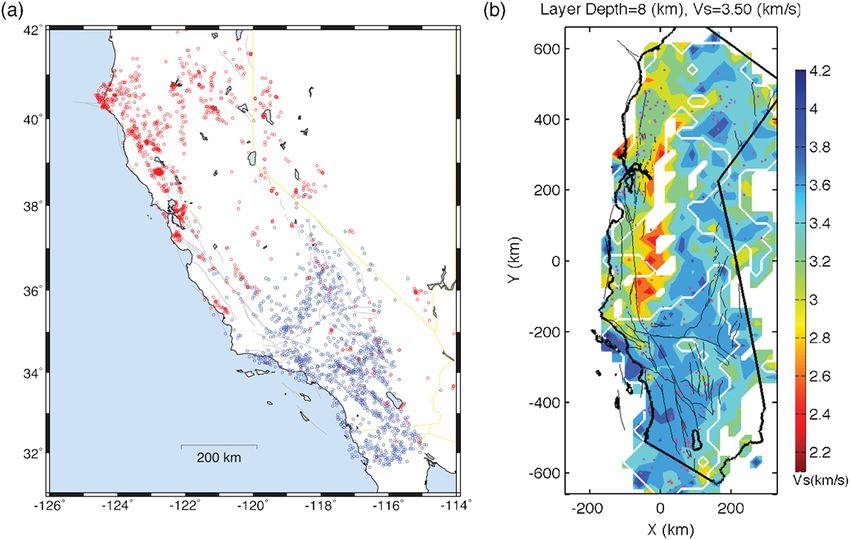
228                       G. Lin, C. H. Thurber, H. Zhang, E. Hauksson, P. M. Shearer, F. Waldhauser, T. M. Brocher, and J. Hardebeck

                                                                        Table 1
                                     A Subset of the Previous Studies on Seismic Velocity Structure in California
                            Study Area                                                  References

                    Coalinga                        Eberhart-Phillips (1990)
                    Coast Ranges                    Eberhart-Phillips (1986); Henstock et al.(1997); Bleibinhaus et al.(2007)
                    Coso geothermal area            Hauksson and Unruh (2007)
                    Coyote Lake                     Thurber (1983)
                    Great Valley                    Hwang and Mooney (1986); Godfrey et al. (1997)
                    Greater Los Angeles basin       Magistrale et al. (1996); Hauksson and Haase (1997); Lutter et al. (1999)
                    Loma Prieta                     Foxall et al. (1993); Thurber et al. (1995); Eberhart-Phillips and Michael (1998)
                    Monterey Bay                    Begnaud et al. (2000)
                    Parkfield region                Eberhart-Phillips and Michael (1993); Thurber et al. (2003, 2006)
                    San Francisco Bay region        Manaker et al. (2005); Hardebeck et al. (2007); Thurber et al (2007)
                    Santa Monica Mountains          Lutter et al. (2004)
                    Sierra Nevada arc               Brocher et al. (1989); Fliedner et al. (1996, 2000); Boyd et al. (2004)
                    Entire southern California      Hauksson (2000); Huang and Zhao (2003); Zhou (2004)

      3D Coarse Model                                                           absolute arrival times for this 3D coarse model. An a priori
                                                                                Moho is not included at this stage, but is introduced later for
     Because of the large spatial scale and amount of data in
                                                                                the finer-scale model. Preliminary inversions were carried
our study, we first solve for a coarse 3D V P model starting
                                                                                out using the tomography algorithm simul2000 (Thurber
with a one-dimensional (1D) velocity model (shown in the
                                                                                and Eberhart-Phillips, 1999). This algorithm simultaneously
small panel of Fig. 2d) for the entire state. This 1D model                     solves for 3D velocity structure and earthquake locations
is based on standard regional 1D velocity models used to lo-                    using the first-arrival times employing an iterative damped-
cate earthquakes by the seismic networks in northern and                        least-squares method. This step was taken for data quality
southern California. The starting model nodes (shown in                         control purposes (i.e., identifying poorly constrained events
Fig. 2d) are uniformly spaced at 30 km intervals in the hor-                    and picks with very high residuals), and to provide formal
izontal directions and extend 570 km in the SW–NE direc-                        but approximate estimates of velocity model resolution
tion and 1320 km in the NW–SE direction. In the vertical                        and uncertainty. After the data quality control step using
direction, the nodes are positioned at 1, 1, 4, 8, 14, 20, 27,                 simul2000, we applied the regional-scale DD tomography
35, and 45 km (relative to mean sea level). We only use                         algorithm, which is more suitable for the large-scale area

                                                                        Table 2
                                         Active-Source Data Sets Included in the Statewide Tomographic Inversion
        Experiment Name                                             Reference                                         Year       No. Shots   No. Stations

   USGS                        Warren (1978)                                                                         1967            9          147
   Geysers-San Pablo Bay       Warren (1981)                                                                         1976            5          135
   Oroville                    Spieth et al. (1981)                                                                  1977            5          118
   Imperial Valley             Kohler and Fuis (1988)                                                                1979           41          932
   Western Mojave Desert       Harris et al.(1988)                                                                   1980           10          245
   Gilroy-Coyote Lake          Mooney and Luetgert (1982)                                                          1980/1981         4          236
   Livermore                   Williams et al. (1999)                                                              1980/1981         3          251
   Great Valley                Murphy (1989); Colburn and Walter (1984)                                            1981/1982         7          221
   San Juan Bautista           Mooney and Colburn (1985)                                                           1981/1982         6          335
   Shasta 1981                 Kohler et al. (1987)                                                                  1981            1          274
   Shasta 1982                 Kohler et al. (1987)                                                                  1982            9          299
   Morro Bay                   Murphy and Walter (1984)                                                              1982            9          230
   Coalinga                    Murphy and Walter (1984)                                                              1983            9          209
   Long Valley                 Meador et al. (1985)                                                                  1983            9          278
   San Luis Obispo             Sharpless and Walter (1988)                                                           1986           10          123
   Loma Prieta                 Brocher et al. (1992)                                                                 1990         2252           16
   San Francisco Bay 1991      Murphy et al.(1992); Kohler and Catchings (1994); Brocher and Pope (1994)             1991            6          300
   PACE 1992                   Fliedner et al. (1996)                                                                1992            5          384
   Southern Sierra             Fliedner et al. (1996)                                                                1993           23         1241
   San Francisco Bay 1993      Catchings et al. (2004)                                                               1993           14          399
   LARSE 1994                  Murphy et al. (1996)                                                                  1994          125          889
   LARSE 1999                  Fuis, Murphy,et al. (2001)                                                            1999           78          925
   Parkfield                   Thurber et al. (2003, 2004); Hole et al. (2006)                                       2003          157          242
   Network                     Northern and Southern California Earthquake Data Center                             1976–2003       270          659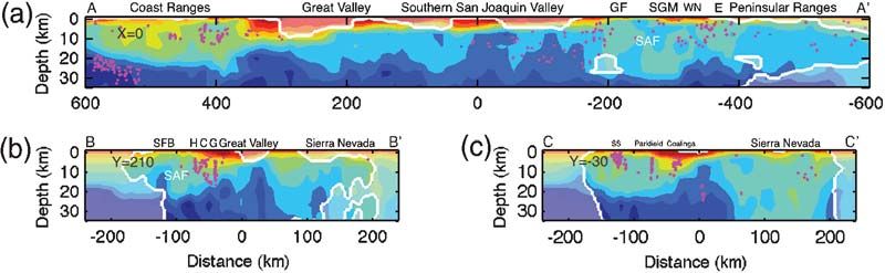
A California Statewide Three-Dimensional Seismic Velocity Model                                                                            229

in this study. To make the inversion more stable, some reg-               deepest layer with a linear gradient for the layers between
ularization method is required, such as smoothing and                     these two layers. In order to start with a conservative 3D
damping. Smoothing regularization provides a minimum-                     model, we removed the low-velocity anomalies in the 3D
feature model that contains only as much structure as can                 coarse model, that is, we require that velocity is initially a
be resolved above the estimated level of noise in the data                monotonically increasing function of depth. The resulting ad-
(Zhang and Thurber, 2003). Damping and smoothing are                      justed 3D model is the starting model for our final P velocity
often selected empirically, by running a series of single-                model. Figure 3a shows the map view of this model at 4 km
iteration inversions with a large range of values, and plotting           depth, with the layer-average velocity values in the inset of
the data variance versus model variance trade-off curves                  Figure 3b. In order to check the effects of the inclusion of
(e.g., Eberhart-Phillips, 1986, 1993). We explored a wide                 the Moho interface on our final results, we compared our
range of damping (from 25 to 1000) and smoothing (from 0                  final model with a model obtained without a Moho (low-
to 1000) to make sure that we looked at the entire trade-off              velocity anomalies are still removed). The two models are
curve instead of a portion of it. The smoothing constraint                quite similar over well-resolved areas and the model differ-
weighting of 100 (same for the horizontal and vertical direc-             ences between the initial models are reduced after the inver-
tions) and the damping parameter of 350 were chosen by                    sion, indicating that our process converges. Ⓔ Table S1 in the
examining these trade-off curves, which produced good
                                                                          electronic edition of BSSA shows a comparison of models
compromises between data misfit and model variance (see
                                                                          with and without the inclusion of a Moho interface.
Ⓔ Figure S1 in the electronic edition of BSSA).
                                                                               In order to use differential times to obtain a finer-scale
                                                                          model given our computer memory limitations, we split the
     3D Starting Model Adjustments                                        entire state into five subregions (Fig. 3a). The adjacent sub-
     Our preliminary modeling work did not include an a                   regions overlap by about 30 km. We use the same depth layers
priori velocity increase at the Moho, but first-arrival body-             as the coarse model. Figure 3b shows the event and station
wave tomography by itself was not capable of imaging sharp                distributions for subregion 1 as an example. For each subre-
discontinuities. Thus, after we obtained the 3D coarse velocity           gion inversion, we use absolute and differential times from
model, we introduced an a priori Moho interface (see Ⓔ                    events inside the subregion (blue circles in Fig. 3b) that are
Figure S2 in the electronic edition of BSSA) from the results             recorded by all the stations (black triangles) and only absolute
of Fuis and Mooney (1990), which was a modification of                    times from events outside of the subregion (pink circles) that
Mooney and Weaver (1989). We set the velocity to 8 km=sec                 are recorded by stations inside of the subregion. In this way,
in the model layer right below the Moho and 8:2 km=sec at the             we improved the resolution of the resulting velocity model for

Figure 3. (a) Map view of the 3D coarse velocity model at 4 km depth and the boundaries of the 5 subregions. (b) Event and station
distribution in the subregion 1 (small panel shows the 1D layer-average velocity). Yellow squares: finer inversion nodes inside of subregion;
green squares: nodes with fixed velocities; blue circles: earthquakes inside of subregion 1; pink circles: earthquakes outside of subregion 1
but recorded by stations inside of the subregion; black triangles: permanent and temporary stations; red stars: active sources (shots and quarry
blasts). Please refer to the text for more details.
230 G. Lin, C. H. Thurber, H. Zhang, E. Hauksson, P. M. Shearer, F. Waldhauser, T. M. Brocher, and J. Hardebeck
the deeper layers due to the inclusion of substantial data at (a) (1) RMS=1.263 s
large epicentral distances. We also include all available explo-
0.15
Normalized Histogram
sion and quarry data for each subregion (red stars). Inside of
each subregion, the horizontal nodes are spaced at 10 km
intervals in the areas with dense data coverage and 20 km
in other areas (yellow squares). The node spacing outside 0.1
of each subregion is 30 km from the coarse model (green
squares). The initial velocity value at each node is computed
from the velocity values at the surrounding eight nodes of the 0.05
coarse initial model using trilinear interpolation as described
in Thurber and Eberhart-Phillips (1999). The velocities out-
side of each subregion are fixed during the inversion of the
inside-subregion velocities. We inverted five local models 0
−2 −1 0 1 2
separately; our final statewide velocity model is a stitched ver- residual (s)
sion of all the five subregion models. The velocities in the (b)
areas of overlap are computed as the average velocities of (2) RMS=0.374 s
the two adjacent subregions. In order to test the robustness 0.15
Normalized Histogram
of our stitching approach, we inverted a model that includes
subregions 1 and 2 and compared the resulting model with the
stitched model. The two models are quite similar with some
0.1
minor differences that are likely caused by different regular-
ization parameters, which are determined individually for
each inversion by examining data variance versus model
variance trade-off curves. 0.05
Model Quality and Resolution
0
The quality of our model can be evaluated by its ability −2 −1 0 1 2
residual (s)
to (1) fit the observed arrival-time data, and (2) produce
accurate locations for onland controlled-source explosions (c) (3) RMS=0.320 s
that have known coordinates. Figure 4 shows a comparison
0.15
Normalized Histogram
of the arrival-time residual distribution before (a) and after
the coarse (b) and final (stitched) (c) 3D velocity inversions
for the entire data set (including controlled sources). The
root-mean-square (rms) misfit is reduced by over a factor 0.1
of 3, from 1.26 sec to 0.37 sec, after the 3D coarse model
inversion, and then to 0.32 sec after the final model inver-
sion. The reason that the fit to absolute times in the subregion
0.05
model inversions is only slightly better than the coarse model
fit is because the purpose of this step is to improve fine-scale
velocity resolution by using differential times. A hierarchical
weighting scheme is applied with greater weight to the 0
−2 −1 0 1 2
absolute data for the first two iterations and greater weight residual (s)
to the differential data for the next four iterations. Note that
most of the improvement of arrival-time fit after the 3D final Figure 4. The arrival-time residual distribution for the entire
model inversion is mainly due to the lower differential time data set (including controlled sources) (a) before 3D velocity inver-
residuals, where the rms misfit of the differential times is sion; (b) after 3D coarse model inversion; (c) after 3D final model
inversion.
reduced from 0.28 sec to 0.11 sec.
We independently located the onshore explosions using
the starting 1D and the coarse and final 3D velocity models are positive when the assigned location is deeper than the
and then calculated the horizontal and vertical location true location and negative when the assigned location is shal-
differences between the relocations and the known true loca- lower than the true location. For the 1D model, the error dis-
tions. Figure 5 shows histograms of shot location accuracy tributions are quite broad, with a mean error of 1.23 km, and
relocated using the starting 1D model compared with the two a standard deviation of 1.08 km horizontally. The vertical
3D models for both horizontal and vertical coordinates. The error distribution has peaks at about 0.6 and 4.5 km, a mean
horizontal location errors are all positive; the vertical errors (absolute) error of 2.19 km, and a standard deviation ofA California Statewide Three-Dimensional Seismic Velocity Model 231
(a) 300 (b)
STD=1.08 km 250 STD=2.38 km
250
200
200
Number
Number
150
150
100
100
50 50
1D 1D
0 0
0 1 2 3 4 5 6 7 0 2 4 6 8 10
Horizontal Error (km) Vertical Error (km)
(c) 300
STD=0.59 km
(d)
250 STD=0.82 km
250
200
200
Number
Number
150
150
100
100
50 50
3D Coarse 3D Coarse
0 0
0 1 2 3 4 5 6 7 0 2 4 6 8 10
Horizontal Error (km) Vertical Error (km)
(e) 300 (f)
STD=0.39 km 250 STD=0.41 km
250
200
200
Number
Number
150
150
100
100
50 50
3D Final 3D Final
0 0
0 1 2 3 4 5 6 7 0 2 4 6 8 10
Horizontal Error (km) Vertical Error (km)
Figure 5. Histograms of the differences between relocations and known true locations for onland explosions. The two columns are for
horizontal and vertical location errors, respectively. (a) and (b) 1D model; (c) and (d) 3D coarse model; (e) and (f) 3D final model.
2.38 km. In contrast, the 3D coarse model error distributions 1D-velocity model cannot account for lateral heterogeneity
are peaked between 0 and 1 km, with mean errors of 0.60 and in velocity structure across all of California. Further, the
0.32 km, and standard deviations of 0.59 and 0.82 km for the 3D final model location error distributions are peaked around
horizontal and vertical errors, respectively. Although this 0.2 km, with mean errors of 0.35 and 0.15 km and standard
model is coarse, the 3D shot relocations are significantly deviations of 0.39 and 0.41 km for the horizontal and vertical
improved, especially in depth. This is because a single errors, respectively. The poorly located shots fall into several232 G. Lin, C. H. Thurber, H. Zhang, E. Hauksson, P. M. Shearer, F. Waldhauser, T. M. Brocher, and J. Hardebeck
categories. One group is distant shots recorded on permanent locities in these shallow layers generally correlate with the
network stations for cases in which we were not able to ob- surface geology. Lower values are observed in basin and
tain the corresponding refraction profile picks. An example is valley areas, such as the Great Valley, southern San Joaquin
the shots from the PACE 1992 project (Fliedner et al., 1996). Valley, Ventura basin, Los Angeles basin, and Imperial Valley,
Others are cases for which data for a particular shot were split whereas relatively higher velocities are present in the moun-
into two separate events, due to the fact that the data were tain ranges, such as the northern Coast Ranges, Transverse
obtained and entered into the database separately. Examples Ranges, Peninsular Ranges, and Sierra Nevada. The correla-
are a number of shots from the Parkfield area and several tion coefficients for the well-resolved areas of these two layers
LARSE shots. Finally, there are a few shots for which only between our model and the NC model are 0.49 and 0.56,
profile picks are available, and the recording geometry is too respectively. The relatively low correlations for these two
poor to constrain the locations adequately. The reduction in layers are mainly due to the low-velocity anomalies in the
relocation errors of about a factor of 2 over the 3D coarse Great Valley and fast anomalies in the Sierra Nevada in our
model indicates that our final model significantly improves model. The lowest velocity anomalies (about 2:9 km=sec)
resolution for the lateral heterogeneities in the 3D velocity appear in the Great Valley and southern San Joaquin Valley.
structure, especially at shallow depths. However, these slow anomalies are at the edge of our well-
To assess the model quality, we performed a restoration resolved areas because of the sparse event distribution in this
and a checkerboard resolution test similar to those in Thurber region. Fairly high-velocity anomalies (∼6:0 km=sec) at 1 km
et al. (2009). In the restoration test, event hypocenters, station depth in the Klamath Mountains and Mount Shasta area are
locations, and synthetic travel times, calculated from the final observed that are consistent with the results from seismic-
inverted model, have the same distribution as the real data. We refraction and gravity data in this area (Zucca et al., 1986; Fuis
followed the same inversion strategies as those for the real et al., 1987), but are not seen in the recent northern California
data and examined the recovering ability of our algorithms. P-wave velocity model by Thurber et al. (2009). This high-
The inverted final model is similar to the true model over velocity body extends to 14 km depth in our model, reaching
well-resolved areas (see Ⓔ Figure S3 in the electronic edition ∼6:5–6:7 km=sec at 4 km, ∼6:7–7:1 km=sec at 8 km, and
of BSSA). In the checkerboard test, the synthetic times are ∼7–7:1 km=sec at 14 km depth, with relatively little structural
computed through the 1D starting velocity model with variations along the north-south direction. These velocities
5% velocity anomalies across three grid nodes. The results are consistent with the conclusion by Fuis et al. (1987),
are shown in Figure S4 (see the Ⓔ electronic edition of BSSA). who argued that an imbricated stack of oceanic rock layers
Note that in this test, we did not include the Moho interface, underlies the Klamath Mountains. Another high-velocity
but still removed low-velocity anomalies as was done for the anomaly zone is apparent at 1 and 4 km depth in the Lake
real data inversion. Some smearing is still seen, part of which Oroville area. The ∼6:8 km=sec velocity at 4 km depth is gen-
is likely due to the interpolation of velocities when obtaining erally consistent with the observations by Spieth et al. (1981)
the starting velocities for subregion models. that the velocity is of the order of 7:0 km=sec at a depth of
5 km. This high-velocity anomaly (∼6:9 km=sec) extends
to 8 km depth in our model. The high velocities at 1 km depth
Final P-Wave Velocity Model in the southern Sierra Nevada area, ranging from 5:2 km=sec
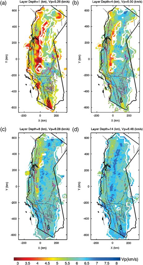
Map Views. Figure 6 shows map view slices through the to 5:8 km=sec, are consistent with the results of Fliedner et al.
resulting tomographic P velocity model. Pink dots in each (1996, 2000). The velocities at 4 km depth are generally high-
figure represent earthquakes relocated within 1 km of each er than those estimated by Thurber et al. (2009) (∼6:0 km=sec
layer depth. The white contours enclose the areas where the compared with ∼5:3 km=sec); our model is more consistent
derivative weight sum (DWS; Thurber and Eberhart-Phillips, with the results based on the active seismic refraction experi-
1999) is greater than 300. Derivative weight sum measures ment by Fliedner et al. (1996, 2000).
the sampling of each node and serves as an approximate In southern California, the correlation coefficients for
measure of resolution (Zhang and Thurber, 2007). Areas these two layers between our model and the SC model are
with DWS values above 300 correspond to well-resolved 0.65 and 0.56, respectively. Note that these coefficients are
areas in the synthetic tests. In the following, we show aver- computed over the resolved areas in the model of Lin et al.
age velocities at each layer computed for these areas. In order (2007), corresponding to the area of X 100 to 200 km
to quantitatively compare our model with previous tomogra- and Y 620 to 100 km. Near-surface velocities in our
phy models, we interpolated the southern and northern model are also relatively high in the western Mojave Desert
California models by Lin et al. (2007) and Thurber et al. in our model. The anomalies are slightly higher than previous
(2009) onto our inversion grids and calculated the correlation results (e.g., Hauksson, 2000; Lin et al., 2007). We think this
coefficients at each layer depth. We will refer to these two may be due to the inclusion of the active-source data in this
models as the SC and NC models in the following. area, which were not used before. In the Imperial Valley area,
Figure 6a,b shows the P-wave velocities in the top two the slowest velocity at 1 km depth is 3:07 km=sec in this
layers of our model. The average velocity values are study, but about 3:6 km=sec at the surface in Lin et al.
5:26 km=sec at 1 km and 6:0 km=sec at 4 km depth. The ve- (2007), who concluded that their model slightly overestimatesA California Statewide Three-Dimensional Seismic Velocity Model 233 Figure 6. Map views of the P-wave velocity model at different depth slices. The white contours enclose the areas where the derivative weight sum is greater than 300. The average velocities are computed over these areas. Pink dots represent relocated earthquakes. Black lines denote coast line and lakes, gray lines rivers and surface traces of mapped faults. (Continued)
234   G. Lin, C. H. Thurber, H. Zhang, E. Hauksson, P. M. Shearer, F. Waldhauser, T. M. Brocher, and J. Hardebeck

                                    Figure 6.     Continued.
A California Statewide Three-Dimensional Seismic Velocity Model 235
the near-surface velocity compared with seismic refraction the results of Thurber et al. (2009), but is slightly slower
results (Fuis et al., 1984). The reduction of this overestimation in the center of the Great Valley. At 27 km depth, the Sierra
indicates that our model has better resolution for near-surface Nevada area shows about 6:0 km=sec low-velocity anoma-
structure. The southern San Joaquin Valley is better resolved lies, but in the same area, the velocity in Thurber et al.
in this new model, which is at the northern boundary of the (2009) is about 6:5 km=sec. Our model extends to 45 km
study area in Lin et al. (2007). depth. Figure 6g,h shows the map views of the last two layers
Figure 6c,d shows map views for 8 and 14 km at 35 km and 45 km depths. Although the model is not re-
depths, with average velocity values of 6:26 km=sec and solved nearly as well as the shallower layers, we are able to
6:46 km=sec, respectively. These layers are the two best- see the low-velocity anomalies in the Sierra Nevada region;
resolved layers in our model because of the abundant seis- the correlation coefficients for these two layers between our
micity at these depths, and the results are generally quite model and the NC model are 0.70 and 0.46, respectively.
compatible with previous tomographic results. At 8 km depth,
a strong velocity contrast is apparent between the Great Valley Cross Sections. We present three cross sections to illumi-
and the Sierra Nevada. At 14 km depth, some of the features nate the large-scale features of the model. One is parallel
we imaged for the shallow layers are reversed, that is, the basin to the San Andreas fault (SAF; X 0 km in the Cartesian co-
and valley areas show relatively high-velocity anomalies and ordinate system), and the other two are perpendicular to the
lower values are present under the mountain ranges. The SAF (Y 210 km and Y 30). A complete set of cross
reversal of the velocity anomalies associated with most of the sections is provided in the Ⓔ electronic edition of BSSA.
major basins is also observed in previous southern and north- In Figure 7 we show the velocity cross sections through
ern California tomography studies (Lin et al., 2007; Thurber the resulting model along the three profiles whose locations
et al., 2009). The correlation coefficients for these two layers are shown in Figure 1.
between our model and the NC model are 0.61 and 0.47, and The X 0 km section in Figure 7a starts in the north-
0.35 and 0.49 with the SC model, respectively. The relatively ern Coast Ranges where intermediate velocities (V P <
poor correlation with the NC model is mainly due to the 6:2 km=sec) extend into the lower crust. At depths greater
slower velocities (∼5%) in the northern Coast Ranges than than 20 km, the seismicity and high velocities of the subduct-
what is observed in the Thurber et al. (2009) model. The ing Gorda Plate are visible. From Y ∼ 350 to 210 km, the
correlation coefficients with the SC model are reduced low near-surface velocities of the Great Valley and southern
compared with the shallower layers. For these two layers, San Joaquin Valley sediments and sedimentary rocks are
our model is generally faster than the Lin et al. (2007) model evident, extending to depths of ∼10 km in the northwest
by about 5% in the basin areas, such as the Ventura basin, Los and to ∼4 km in the southeast. High-velocity rocks (V P ∼
Angeles basin, and Imperial Valley. 6:5 km=sec) of the underlying Great Valley ophiolite body
Map views for the 20 and 27 km depth layers are shown are present throughout this part of the section. The section
in Figure 6e,f, with average velocity values of 6:81 km=sec crosses the Garlock fault (Y ∼ 210 km) and the SAF
and 7:28 km=sec, respectively. The correlation coefficients (Y ∼ 255 km), where upper and midcrustal velocities are
for these two layers between our model and the NC model relatively low (V P < 6:3 km=sec), and then cuts through the
are 0.65 and 0.72, respectively. The resolution of the south- San Gabriel Mountains (SGM) and Peninsular Ranges where
ern California model by Lin et al. (2007) is poor below the upper crust velocities are relatively high (V P >
17 km depth, so we focus on the comparison in northern 6:2 km=sec) at shallow depths. Beneath the SAF and SGM,
California. At 20 km depth, the model is consistent with a strong low-velocity zone is apparent, as identified in
Figure 7. Cross sections of the absolute P-wave velocity along the three profiles shown in Figure 1. Again, the pink dots represent
relocated earthquakes and the white contours enclose the area where the derivative weight sum is less than 300. Color scale is the same as in
Figure 6. Abbreviations: C, Calaveras fault; E, Elsinore fault; GF, Garlock fault; G, Greenville fault; H, Hayward fault; SAF, San Andreas
fault; SFB, San Francisco Bay; SGM, San Gabriel Mountains; SS, San Simeon; WN, Whittier Narrows.236 G. Lin, C. H. Thurber, H. Zhang, E. Hauksson, P. M. Shearer, F. Waldhauser, T. M. Brocher, and J. Hardebeck
previous studies in this area, which has been interpreted to S-Wave Velocity Model
indicate fluids (e.g., Ryberg and Fuis, 1998; Fuis et al.,
2000). Although S-wave velocity models in northern California
The section in Figure 7b cuts across the seismically are available from ambient noise and surface wave data
quiet southern San Francisco (SF) Peninsula and SF Bay (e.g., Yang et al., 2008), there is no 3D model based on
regional network data. In this study, we use the S first-arrival
(X 120 to 90 km) and then reaches the seismically
times from the SCSN and USArray to solve for a V S model.
active Hayward, Calaveras, and Greenville faults beneath
Note that these data are different from those used for the V P
the East Bay (X 70 to 30 km). The section then enters
model. Figure 8a shows the 1020 SCSN and 1292 USArray
the Great Valley, where the high-velocity basement, thought
events with at least 4 P and 4 S picks. Due to the sparse
to be ophiolite (e.g., Godfrey et al., 1997), shallows to the
distribution of the data, we use the velocity inversion nodes
northeast (X 30 to 50 km). After that, the section
of the 3D coarse V P model (i.e., 30 by 30 km horizontal node
enters the Sierra Nevada where a thicker crust with a velocity spacing). The starting S velocities are derived from our
of ∼6:2 km=sec extends to 32 km depth. The section in resolved V P model and a constant V P =V S of 1.73. The re-
Figure 7c passes through the seismic activity of San Simeon solution estimated by the DWS values is quite poor. In order
(X 120 km), Parkfield (X 75 km), and Coalinga to test the robustness of the S model, we also start with the S
(X 30 km). Even with the 10 km model gridding, the velocity values from the ambient noise and teleseismic
velocity contrast across the San Andreas at Parkfield is multiple-plane-wave tomography results by Yang et al.
evident (southwest side faster, e.g., Thurber et al., 2006). (2008). The well-resolved part agrees with the results starting
In this section as well, the high-velocity Great Valley ophio- with the constant V P =V S , indicating that the model is rela-
lite body is evident with a predominantly southwestern dip of tively robust. Figure 8b shows the map view of our resolved
its upper surface, consistent with potential field data (Jachens V S model at 8 km depth. The white contours enclose the area
et al., 1995). At X ∼ 50 km, we see a transition to the slower, where the derivative weight sum is greater than 100. We also
thicker crust of the Sierra Nevada. compared our V P and V S models to the empirical V P V S
Figure 8. (a) Event distribution for V S model. The red and blue circles represent the events from the USArray and SCSN, respectively.
(b) Map view of our resolved V S model at 8 km depth. Areas where the derivative weight sum is greater than 100 are shown. The average
velocity is computed over these areas. The pink dots represent relocated earthquakes.A California Statewide Three-Dimensional Seismic Velocity Model 237
relation of Brocher (2005). This relation is derived from a by applying the SIMULPS algorithm (Thurber, 1983, 1993;
diverse dataset, including wireline borehole logs, vertical Eberhart-Phillips, 1990; Evans et al., 1994) to absolute
seismic profiles, laboratory measurements, and seismic arrival times for composite events. We also calculated the
tomography models, and can be used to infer V S for the correlation coefficients, which are 0.67, 0.56, 0.36, 0.54,
entire Earth’s crust from V P . Using the layer-average P and 0.69 for the top five layers, between our model and
velocities as inputs, we obtained the corresponding empirical the SCEC unified velocity model (Version 4, Magistrale et al.,
S velocities. Our comparison indicates that the tomography- 2000). Note that the SCEC model is based on geotechnical
based V S results are faster than predicted by the empirical borehole seismic velocity data and the regional tomographic
relation at 1 and 35 km depth, and lower than expected at model of Hauksson (2000), which is also obtained by apply-
8 km depth. Due to the poor resolution of this model, we ing the SIMULPS algorithm. The slightly better correlation at
do not attempt to solve for Poisson’s ratio and other param- 1 km depth is due to the low-velocity anomalies in the basin
eters that depend on V P =V S values. A complete set of map areas. Our new model is generally consistent with these pre-
views and cross sections of our S-wave model is provided in vious results. The improved resolution of our model in near-
the Ⓔ electronic edition of BSSA). surface layers over the previous California tomographic
models is mainly due to the large amount of active-source
Discussion data in this study.
The goal of this study is not to replace the previous
Our model is the first 3D seismic velocity model for the tomographic models in California that have more detail than
entire state of California based on local and regional arrival- can be resolved by our data and grid spacing, but to image
time data. It has improved areal coverage compared with the the entire state of California at a regional scale, to reveal
previous northern and southern California models, and ex- some features that are difficult to resolve in local studies,
tends to greater depth due to the inclusion of substantial data and to provide the geophysical community with a velocity
at large epicentral distances. The combination of northern, model that should be useful for regional-scale studies, such
southern, and central California data sets results in better- as regional waveform modeling. The model is available in
resolved velocity structure at the study boundaries of pre- the Ⓔ electronic edition of BSSA.
vious tomographic models, such as the San Joaquin Valley
and southern Sierra Nevada. Because of the 10 km horizontal
grid spacing in our model inversion, which is larger than the Conclusions
distance cutoff of most waveform cross-correlation calcula-
tions (≤ 5 km), we did not apply any differential times from We have developed statewide body-wave tomography
cross-correlation in this study. There may be some finer-scale models (P and S) for California using absolute and differen-
structures that are not resolved due to the data and grid spa- tial arrival times from earthquakes, controlled sources, and
cing used in our model. We compared our model with some quarry blasts. By merging the data sets from networks
results based on refraction and/or reflection data. Our model in northern, southern, and coastal central California and
generally agrees with most of the studies, such as in the Dia- USArray, we have achieved relatively complete coverage
blo and Gabilan Ranges (Steppe and Robert, 1978; Walter of the entire state for V P. By including a large amount of
and Mooney, 1982), the Coyote Lake (Mooney and Luetgert, active-source data in this study, we obtained improved res-
1982), the Long Valley (Luetgert and Mooney, 1985), the olution in near-surface layers over the previous California
San Francisco Bay area (Holbrook et al., 1996), the southern tomographic models, especially in the largest sedimentary
Sierra (Fliedner et al., 1996), and the Mojave Desert (Fuis, basins, such as the Great Valley, the Imperial Valley, and
Ryberg, et al., 2001); but slightly overestimates near-surface the Los Angeles basin. At 8 km depth, there is a clear north
velocity values in some basins and valleys, such as in the to south increase in the average velocity of the Coast Range
Imperial Valley (McMechan and Mooney, 1980; Fuis et al., Mountains extending from the Mendocino Triple Junction to
1984), the Great Valley (Colburn and Mooney, 1986), the the border with Mexico. At 14 and 20 km depths, the basin
Livermore area (Meltzer et al., 1987), and the greater Los and valley areas show relatively high-velocity anomalies,
Angeles basin (Fuis, Ryberg, et al., 2001b). with lower velocities present under the mountain ranges.
The differences between this statewide velocity model The Great Valley ophiolite body and the subducting Gorda
and previous regional-scale models are due to several factors, Plate are evident from the cross sections. Low-velocity
such as data sets, grid spacing (cell size), tomographic algo- anomalies in the Sierra Nevada exist from midcrustal to
rithms, and inversion parameters (e.g., damping, smoothing, greater depths; the slow velocity root over this area is the
and residual weighting). The model is very similar to the largest anomaly at 35 km depth. Our model provides a rea-
recent northern California model by Thurber et al. (2009) sonable fit to the data and relocates explosions, treated as
for the middle to lower crust because the two studies use earthquakes, with an absolute accuracy of better than a
the same type of data sets (both absolute and differential kilometer. Thus, it should be useful for producing a state-
times) and inversion algorithm (tomoFDD), whereas the wide earthquake location catalog based on a single velocity
southern California model by Lin et al. (2007) is derived model.238 G. Lin, C. H. Thurber, H. Zhang, E. Hauksson, P. M. Shearer, F. Waldhauser, T. M. Brocher, and J. Hardebeck
Data and Resources Colburn, R. H., and A. W. Walter (1984). Data report for two seismic-
refraction profiles crossing the epicentral region of the 1983 Coalinga,
Active-source data used in this study were collected from California earthquakes, U.S. Geol. Surv. Open-File Rept. 84-643,
published studies listed in the references. Catalog picks were 58 pp.
Eberhart-Phillips, D. (1986). Three-dimensional velocity structure in the
obtained from the USArray, the Northern California Earth- northern California Coast Ranges from inversion of local earthquake
quake Data Center (NCEDC), and the Southern California arrival times, Bull. Seismol. Soc. Am. 76, 1025–1052.
Earthquake Data Center (SCEDC) and originate principally Eberhart-Phillips, D. (1990). Three-dimensional P and S velocity structure in
from the Northern California Seismic Network (NCSN) and the Coalinga region, California, J. Geophys. Res. 95, 15,343–15,363.
Southern California Seismic Network (SCSN). Some figures Eberhart-Phillips, D. (1993). Local earthquake tomography: earthquake
source regions, in Seismic Tomography: Theory and Practice,
were made using the public domain Generic Mapping Tools H. M. Iyer and K. Hirahara (Editors), Chapman and Hall, London,
software (Wessel and Smith, 1991). 613–643.
Eberhart-Phillips, D., and A. J. Michael (1993). Three-dimensional velocity
structure, seismicity, and fault structure in the Parkfield region, central
Acknowledgments California, J. Geophys. Res. 98, 15737–15758.
Eberhart-Phillips, D., and A. J. Michael (1998). Seismotectonics of the
We thank the U.S. Geological Survey (USGS) and Caltech staff for
Loma Prieta, California, region determined from three-dimensional
maintaining the NCSN and SCSN, and the IRIS Data Management Center
V P , V P =V S , and seismicity, J. Geophys. Res. 103, 21,099–21,120.
for making USArray data available. R. Catchings,C. Evangelidis, A. Frankel,
Evans, J. R., D. Eberhart-Phillips, and C. H. Thurber (1994). User’s manual
G. Fuis, S. Hartzell, W. Kohler, A. Lindh, J. Murphy, D. O’Connell, and
for SIMULPS12 for imaging V P and V P =V S : A derivative of the
T. Parsons contributed first-arrival times and receiver and source locations
“Thurber” tomographic inversion SIMUL3 for local earthquakes
for active-source experiments in the study area. We thank W.-X. Du for
and explosions, U.S. Geol. Surv. Open-File Rept. 94-431.
his effort to assemble the northern California active-source data set into a con-
Flanagan, M. P., S. C. Myers, and K. D. Koper (2007). Regional travel-time
sistent form and Y. Yang for providing his ambient noise tomography model.
uncertainty and seismic location improvement using a three-
This work is supported by the National Earthquake Hazards Reduction pro-
dimensional a priori velocity model, Bull. Seismol. Soc. Am. 97,
gram, under USGS awards 07HQGR0038, 07HQGR0045, 07HQGR0047,
804–825.
07HQGR0050, 08HQGR0032, 08HQGR0039, 08HQGR0042 and
Fliedner, M. M., S. L. Klemperer, and N. I. Christensen (2000). Three-
08HQGR0045, and the National Mapping Programs of the USGS. The views
dimensional seismic model of the Sierra Nevada arc, California,
and conclusions contained in this document are those of the authors and
and its implications for crustal and upper mantle composition, J. Geo-
should not be interpreted as necessarily representing the official policies,
phys. Res. 105, 10899–10922.
either expressed or implied, of the U.S. government.
Fliedner, M. M., S. Ruppert, and the Southern Sierra Nevada Continental
Dynamics Working Group (1996). Three-dimensional crustal structure
of the southern Sierra Nevada from seismic fan profiles and gravity
References
modeling, Geology 24, 367–370.
Begnaud, M. L., K. C. McNally, D. S. Stakes, and V. A. Gallardo (2000). A Foxall, W., A. Michelini, and T. V. McEvilly (1993). Earthquake travel time
crustal velocity model for locating earthquakes in Monterey Bay, tomography of the southern Santa Cruz Mountains: Control of fault
California, Bull. Seismol. Soc. Am. 90, 1391–1408, doi 10.1785/ rupture by lithological heterogeneity of the San Andreas Fault zone,
0120000016. J. Geophys. Res. 98, 17,691–17,710.
Bleibinhaus, F., J. A. Hole, T. Ryberg, and G. S. Fuis (2007). Structure of the Fuis, G., and W. D. Mooney (1990). Lithospheric structure and tectonics
California Coast Ranges and San Andreas Fault at SAFOD from seis- from seismic-refraction and other data, The San Andreas Fault System,
mic waveform inversion and reflection imaging, J. Geophys. Res. 112, California: U.S. Geol. Surv. Prof. Paper 1515, 207–236.
B06315, doi 10.1029/2006JB004611. Fuis, G. S., W. D. Mooney, J. H. Healy, G. A. McMechan, and W. J. Lutter
Boyd, O. S., C. H. Jones, and A. F. Sheehan (2004). Foundering lithosphere (1984). A seismic refraction survey of the Imperial Valley region,
imaged beneath the southern Sierra Nevada, California, USA, Science California, J. Geophys. Res. 89, 1165–1190.
305, 660–662. Fuis, G. S., J. M. Murphy, D. A. Okaya, R. W. Clayton, P. M. Davis,
Brocher, T. M. (2005). Empirical relations between elastic wavespeeds and K. Thygesen, S. A. Baher, T. Ryberg, M. L. Benthien, G. Simila,
density in the Earth’s crust, Bull. Seismol. Soc. Am. 95, 2081–2092. J. T. Perron, A. K. Yong, L. Reusser, W. J. Lutter, G. Kaip, M. D. Fort,
Brocher, T. M., and D. C. Pope (1994). Onshore-offshore wide-angle seismic I. Asudeh, R. Sell, J. R. Vanschaack, E. E. Criley, R. Kaderabek,
recordings of the San Francisco Bay Area Seismic Imaging W. M. Kohler, and N. H. Magnuski (2001). Report for borehole
eXperiment (BASIX); data from the Northern California Seismic explosion data acquired in the 1999 Los Angeles region seismic
Network, U.S. Geol. Surv. Open-File Rept. 94-156. experiment (LARSE II), southern California. I. Description of the
Brocher, T. M., P. E. Hart, and S. Carle (1989). Feasibility study of the survey, U.S. Geol. Surv. Open-File Rept. 01-408, 82 pp.
seismic reflection method in Amargosa Desert, Nye County, Nevada, Fuis, G. S., T. Ryberg, N. J. Godfrey, D. A. Okaya, and J. M. Murphy
U.S. Geol. Surv. Open-File Rept. 89-133, 150 pp. (2001b). Crustal structure and tectonics from the Los Angeles basin
Brocher, T. M., M. J. Moses, and S. D. Lewis (1992). Wide-angle seismic to the Mojave Desert, southern California, Geology 29, 15–18.
recordings obtained during seismic reflection profiling by the S. P. Lee Fuis, G. S., T. Ryberg, N. J. Godfrey, D. A. Okaya, W. J. Lutter, J. M. Murphy,
offshore the Loma Prieta epicenter, U.S. Geol. Surv. Open-File Rept. and V. E. Langenheim (2000). Crustal structure and tectonics of the San
92-245, 63 pp. Andreas Fault in the Central Transverse Ranges/Mojave Desert Area,
Catchings, R. D., M. R. Goldman, C. E. Steedman, and G. Gandhok (2004). 3rd Conference on Tectonic Problems of the San Andreas Fault System.
Velocity models, first-arrival travel times, and geometries of 1991 and Fuis, G. S., J. J. Zucca, W. D. Mooney, and B. Milkereit (1987). A geologic
1993 USGS land-based controlled-source seismic investigations in the interpretation of seismic-refraction results in northeastern California,
San Francisco Bay Area, California: In-line Shots, U.S. Geol. Surv. Geol. Soc. Am. Bull. 98, 53–65.
Open-File Rept., 2004-1423, 32 pp. Godfrey, N. J., B. C. Beaudoin, and S. L. Klemperer (1997). Ophiolitic base-
Colburn, R. H., and W. D. Mooney (1986). Two-dimensional velocity ment to the Great Valley forearc basin, California, from seismic and
structure along the synclinal axis of the Great Valley, California, Bull. gravity data: Implications for crustal growth at the North American
Seismol. Soc. Am. 76, 1305–1322. continental margin, Geol. Soc. Am. Bull. 109, 1536–1562.A California Statewide Three-Dimensional Seismic Velocity Model 239
Hardebeck, J. L., A. J. Michael, and T. M. Brocher (2007). Seismic velocity Desert, California: Results from the Los Angeles Region Seismic
structure and seismotectonics of the eastern San Francisco Bay region, Experiment, J. Geophys. Res. 104, 25,543–25,565.
California, Bull. Seismol. Soc. Am. 97, 826–842. Magistrale, H., S. Day, R. W. Clayton, and R. Graves (2000). The SCEC
Harris, R., A. W. Walter, and G. S. Fuis (1988). Data report for the 1980– southern California reference three-dimensional seismic velocity
1981 seismic-refraction profiles in the western Mojave Desert, model version 2, Bull. Seismol. Soc. Am. 90, S65–S76.
California, U.S. Geol. Surv. Open-File Rept. 88-580, 65 pp. Magistrale, H., K. McLaughlin, and S. Day (1996). A geology-based 3D
Hauksson, E. (2000). Crustal structure and seismicity distribution adjacent to velocity model of the Los Angeles basin sediments, Bull. Seismol.
the Pacific and North America plate boundary in southern California, Soc. Am. 86, 1161–1166.
J. Geophys. Res. 105, 13,875–13,903. Manaker, D. M., A. J. Michael, and R. Burgmann (2005). Subsurface struc-
Hauksson, E., and J. S. Haase (1997). Three-dimensional V P and V P =V S ture and kinematics of the Calaveras–Hayward Fault stepover from
velocity models of the Los Angeles basin and central Transverse three-dimensional V P and seismicity, San Francisco Bay region,
Ranges, California, J. Geophys. Res. 102, 5423–5453. California, Bull. Seismol. Soc. Am. 95, 446–470.
Hauksson, E., and J. Unruh (2007). Regional tectonics of the Coso geother- McMechan, G. A., and W. D. Mooney (1980). Asymptotic ray theory and
mal area along the intracontinental plate boundary in central eastern synthetic seismograms for laterally varying structures: Theory and
California: Three-dimensional V P and V P =V S models, spatial- application to the Imperial Valley, California, Bull. Seismol. Soc.
temporal seismicity patterns, and seismogenic deformation, J. Geo- Am. 70, 2021–2035.
phys. Res. 112, B06309, doi10.1029/2006JB004721. Meador, P. J., D. P. Hill, and J. H. Luetgert (1985). Data report for the July–
Hellweg, M., D. Given, E. Hauksson, D. Neuhauser, D. Oppenheimer, and August 1983 seismic-refraction experiment in the Mono Craters–Long
A. Shakal (2007). The California Integrated Seismic Network, Eos Valley region, California, U.S. Geol. Surv. Open-File Rept. 85-708,
Trans. AGU 88, Jt. Assem. Suppl., Abstract S33C-07. 70 pp.
Henstock, T. J., A. Levander, and J. A. Hole (1997). Deformation in the Meltzer, A. S., A. R. Levander, and W. D. Mooney (1987). Upper crustal
lower crust of the San Andreas Fault System in northern California, structure, Livermore Valley and vicinity, California coast ranges, Bull.
Science 278, 650–653. Seismol. Soc. Am. 77, 1655–1673.
Holbrook, W. S., T. M. Brocher, U. S. ten Brink, and J. A. Hole (1996). Mooney, W. D., and R. H. Colburn (1985). A seismic-refraction profile
Crustal structure of a transform plate boundary: San Francisco Bay across the San Andreas, Sargent, and Calaveras faults, west-central
and the central California continental margin, J. Geophys. Res. 101, California, Bull. Seismol. Soc. Am. 75, 175–191.
22,311–22,334. Mooney, W. D., and J. H. Luetgert (1982). A seismic refraction study of the
Hole, J. A., T. Ryberg, G. S. Fuis, F. Bleibinhaus, and A. K. Sharma (2006). Santa Clara Valley and southern Santa Cruz Mountains, west-central
Structure of the San Andreas Fault zone at SAFOD from a California, Bull. Seismol. Soc. Am. 72, 901–909.
seismic refraction survey, Geophys. Res. Lett. 33, doi 10.1029/ Mooney, W. D., and C. S. Weaver (1989). Regional crustal structure
2005GL025194. and tectonics of the pacific coastal states; California, Oregon and
Huang, J.-l., and D. Zhao (2003). P-wave tomography of crust and upper Washington, in Geophysical Framework of the Continental United
mantle under southern California: Influence of topography of Moho States, I. C. Pakiser and W. D. Mooney (Editors), Geol. Soc. Am.
discontinuity, Acta Seismologica Sinica 16, 577–587. Mem., 172, 129–161.
Hwang, L. J., and W. D. Mooney (1986). Velocity and Q structure of Murphy, J. M. (1989). Data report for the Great Valley, California, axial
the Great Valley, California, based on synthetic seismogram seismic refraction profiles, U.S. Geol. Surv. Open-File Rept. 89-
modeling of seismic refraction data, Bull. Seismol. Soc. Am. 76, 494, 36 pp.
1053–1067. Murphy, J. M., and A. W. Walter (1984). Data report for a seismic-refraction
Jachens, R. C., A. Griscom, and C. W. Roberts (1995). Regional extent of investigation: Morro Bay to the Sierra Nevada, California, U.S. Geol.
Great Valley basement west of the Great Valley, California: Surv. Open-File Rept. 84-642, 37 pp.
Implications for extensive tectonic wedging in the California Coast Murphy, J. M., R. D. Catchings, W. M. Kohler, G. S. Fuis, and D. Eberhart-
Ranges, J. Geophys. Res. 100, 12,769–12,790. Phillips (1992). Data report for 1991 active-source seismic profiles in
Kohler, W. M., and R. D. Catchings (1994). Data report for the 1993 seismic the San Francisco Bay area, U.S. Geol. Surv. Open-File Rept. 92-570,
refraction experiment in the San Francisco Bay Area, California, U.S. 45 pp.
Geol. Surv. Open-File Rept. 94-241, 71 pp. Murphy, J. M., G. S. Fuis, T. Ryberg, D. A. Okaya, E. E. Criley, M. L.
Kohler, W. M., and G. S. Fuis (1988). Data report for the 1979 seismic- Benthien, M. Alvarez, I. Asudeh, W. M. Kohler, G. N. Glassmoyer,
refraction experiment in the Imperial Valley region, California, U.S. M. C. Robertson, and J. Bhowmik (1996). Report for explosion data
Geol. Surv. Open-File Rept. 88-255, 96 pp. acquired in the 1994 Los Angeles Region Seismic Experiment
Kohler, W. M., G. S. Fuis, and P. A. Berge (1987). Data report for the 1978– (LARSE 94), Los Angeles, California, U.S. Geol. Surv. Open-File
1985 seismic-refraction surveys in northeastern California, U.S. Geol. Rept. 96-536, 120 pp.
Surv. Open-File Rept. 87-625, 99 pp. Ryberg, T., and G. S. Fuis (1998). The San Gabriel Mountains bright reflec-
Lin, G., P. M. Shearer, E. Hauksson, and C. H. Thurber (2007). A three- tive zone: Possible evidence of young mid-crustal thrust faulting in
dimensional crustal seismic velocity model for southern California southern California, Tectonophysics 286, 31–46.
from a composite event method, J. Geophys. Res. 112, doi Sharpless, S. W., and A. W. Walter (1988). Data report for the 1986 San Luis
10.1029/2007JB004977. Obispo, California, seismic refraction survey, U.S. Geol. Surv.
Luetgert, J. H., and W. D. Mooney (1985). Crustal refraction profile of the Open-File Rept. 88-35, 48 pp.
Long Valley caldera, California, from the January 1983 Mammoth Spieth, M. A., D. P. Hill, and R. J. Geller (1981). Crustal structure in the
Lakes earthquake swarm, Bull. Seismol. Soc. Am. 75, 211–221. northwestern foothills of the Sierra Nevada from seismic refraction
Lutter, W. J., G. S. Fuis, T. Ryberg, D. A. Okaya, R. W. Clayton, P. M. Davis, experiments, Bull. Seismol. Soc. Am. 71, 1075–1087.
C. Prodehl, J. M. Murphy, V. E. Langenheim, M. L. Benthien, Steppe, A. J., and C. S. Robert (1978). P-velocity models of the southern
N. J. Godfrey, N. I. Christensen, K. Thygesen, C. H. Thurber, G. Simila, Diablo Range, California, from inversion of earthquake and explosion
and G. R. Keller (2004). Upper crustal structure from the Santa Monica arrival times, Bull. Seismol. Soc. Am. 68, 357–367.
Mountains to the Sierra Nevada, Southern Californnia: Tomographic Thurber, C. H. (1983). Earthquake locations and three-dimensional crustal
results from the Los Angeles regional seismic experiment, phase II structure in the Coyote Lake area, central California, J. Geophys. Res.
(LARSE II), Bull. Seismol. Soc. Am. 94, 619–632. 88, 8226–8236.
Lutter, W. J., G. S. Fuis, C. H. Thurber, and J. Murphy (1999). Tomographic Thurber, C. H. (1993). Local earthquake tomography: Velocities and
images of the upper crust from the Los Angeles basin to the Mojave V P =V S -theory, in Seismic Tomography: Theory and Practice,You can also read