Shape and rate of movement of the invasion front of Xylella fastidiosa spp. pauca in Puglia - Nature
←
→
Page content transcription
If your browser does not render page correctly, please read the page content below
www.nature.com/scientificreports
OPEN Shape and rate of movement
of the invasion front of Xylella
fastidiosa spp. pauca in Puglia
David Kottelenberg1*, Lia Hemerik1, Maria Saponari2 & Wopke van der Werf3
In 2013, Xylella fastidiosa spp. pauca was first reported in Puglia, Italy, causing the olive quick decline
syndrome (OQDS). Since then the disease has spread, prompting the initiation of management
measures to contain the outbreak. Estimates of the shape of the disease front and the rate of area
expansion are needed to inform management, e.g. the delineation of buffer zones. However, empirical
estimates of the invasion front and the rate of spread of OQDS are not available. Here, we analysed
the hundreds of thousands of records of monitoring data on disease occurrence in Puglia to estimate
the shape of the invasion front and the rate of movement of the front. The robustness of estimation
was checked using simulation. The shape of the front was best fitted by a logistic function while using
a beta-binomial error distribution to model variability around the expected proportion of infected
trees. The estimated rate of movement of the front was 10.0 km per year (95% confidence interval:
7.5–12.5 km per year). This rate of movement is at the upper limit of previous expert judgements.
The shape of the front was flatter than expected. The fitted model indicates that the disease spread
started approximately in 2008. This analysis underpins projections of further disease spread and the
need for preparedness in areas that are still disease free.
There is a crisis in Puglia, southern Italy, due to a new plant disease caused by bacterium Xylella fastidiosa spp.
pauca. The bacterium causes a disease that is named olive quick decline syndrome (OQDS)1.
It is estimated that 8,000 hectares of olive orchards were affected by the bacterium in 2013, the year of first
reporting of the d isease1–3. In December 2014, one year after first report, the known infected area had almost
tripled4. OQDS severely impacts the local economy of the Puglia region as the symptoms progress rapidly on
the trees, which become unproductive and eventually die. In affected areas, production and movement of plants
for planting is regulated, causing a decline in income from nursery production5,6.
Olives are symbolic trees for the region and the olive orchards are part of the local landscape and cultural
heritage6. The loss of often centuries-old trees greatly affects the cultural heritage and attractiveness of the region.
Farms have been the property and livelihood of families for many years and generations, and the locals find a lot
of pride in their farms. Although these consequences of the invasion are hard to monetize, the impacts are large.
A campaign to monitor disease spread and intercept new advanced foci has been in place in Puglia since
November 2013. Samples have been taken from olive trees and other known susceptible host species to assess
the presence of X. fastidiosa. The sampling strategy is based on the delineation of three so-called “demarcated
areas”7: (1) the infected zone, which is the area that contains all known infected trees; (2) the containment zone,
which is the 20 km wide northern part of the infected zone where infections are regularly found and specific
control operations are mandatory; and (3) the buffer zone, which is the 10 km wide disease free area immedi-
ately outside the infected zone where strict measures are taken to prevent the disease from establishing. The
demarcation of the areas is based on the prescriptions of the EU Decision 2015/789, recently amended by the
EU Regulation 2020/1201, and is continuously updated in relation to the results of each monitoring campaign
(Fig. 1). As the sampling follows the requirements of regulations, which have been updated through time, the
sampling pattern is very heterogeneous in space (Fig. 2) and the number of samples as a function of distance to
the presumed origin of the disease outbreak, Gallipoli, varies substantially from year to year (Fig. 3). Given the
primary objective of the surveillance program (i.e. early detection of potential new infections at the forefront
of the invasion) sampling and testing have been implemented preferentially in a specific band of the region: the
buffer zone in which the bacterium is supposedly not yet present, and in the containment zone, 20 km wide,
1
Wageningen University, Biometris, P.O. Box 16, 6700 AA Wageningen, The Netherlands. 2Consiglio
Nazionale delle Ricerche, Istituto per la Protezione Sostenibile Delle Piante, Bari, via Amendola 122/D, Bari,
Italy. 3Wageningen University and Research, Centre for Crop Systems Analysis, P.O. Box 430, 6700 AA Wageningen,
The Netherlands. *email: david.kottelenberg@gmail.com
Scientific Reports | (2021) 11:1061 | https://doi.org/10.1038/s41598-020-79279-x 1
Vol.:(0123456789)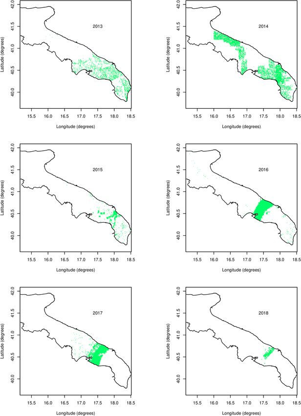
www.nature.com/scientificreports/
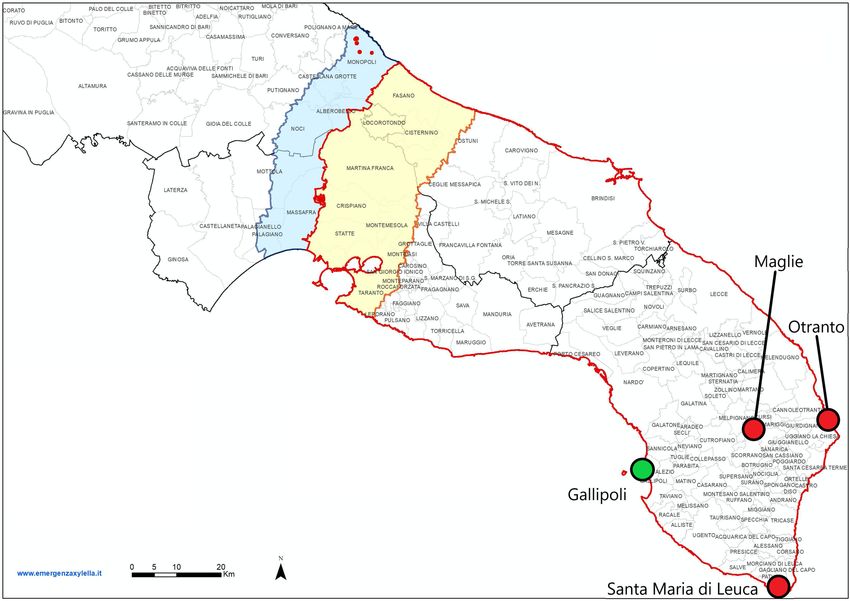
Figure 1. Demarcated areas in October 2020 in the Puglia region, southern Italy. The red outlined region is
the whole infected zone. Within the infected zone, the yellow region is the containment zone, where all infected
plants must be removed, and all host plants within a 100 m radius of the infected plants are tested. The blue
region is the buffer zone, where every infected plant found should be removed, as well as all host plants within a
100 m radius of the infected plant. The red dots in the blue region are newly found infected plants in the buffer
zone for which the demarcated zones have not been updated yet. The green dot is the town of Gallipoli, the
presumed origin of the outbreak of X. fastidiosa in Puglia. The red dots are the towns of Maglie, Otranto, and
Santa Maria di Leuca. These locations are used as alternative origins of the outbreak in sensitivity analyses on
the point of origin. The image was obtained from https://www.emergenzaxylella.it.
located between the heavily infected area and the buffer zone. After 2015, a very limited number of trees have
been monitored in the area declared infected, and the monitored territories varied according to the continuous
change in the demarcation of the areas as consequence of findings of new outbreaks. There is also a large dif-
ference in the number of samples taken each calendar year (Fig. 3). The irregularity of the sampling pattern in
space, and the large differences between years in where samples were taken, make the analysis of the data chal-
lenging. The irregularity of the sampling strategy could result in a biased analysis result when using these data.
However, solving the problem of estimation with such irregular data is important, because such irregularity is
the rule rather than the exception in datasets of disease i nvasions8–10.
Several models have been developed to analyse and predict the spread of X. fastidiosa. White et al.11 modelled
the spread of X. fastidiosa using a spatially explicit simulation model. The model was calibrated on the spatial data
on disease presence from surveys. This model was used to make calculations on the optimal width of the buffer
zone and make calculations on disease survey and detection efficiency and inform management. Soubeyrand
et al.12 developed an SIR model (susceptible, infectious, recovered for the three compartments of the model) to
describe the epidemiology of X. fastidiosa in southern France. They found that the introduction of X. fastidiosa
in France could have occurred around 1985, suggesting there may be hidden compartments in which the bacte-
rium was not detected for a long t ime12. Hidden compartments might exist for other X. fastidiosa introductions
as well, implying that the first detection of the bacterium could be many years after its introduction. The model
of Soubeyrand et al.12 focuses on disease progress in time and ignores spatial aspects. Strona et al.13 developed
an epidemic network model. They found that in the orchard network in Puglia many nodes have many con-
nections, as opposed to most other real-world networks. This implies that containment of the bacterial spread
is very challenging. Finding practical solutions to cope with the infections in the heavily infected area is one of
the research priorities.
Scientific Reports | (2021) 11:1061 | https://doi.org/10.1038/s41598-020-79279-x 2
Vol:.(1234567890)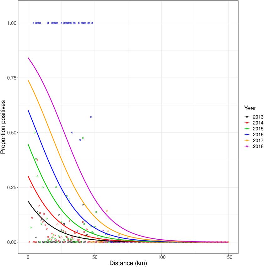
www.nature.com/scientificreports/

                                  Figure 2.  The sampling pattern in the Puglia region per year, 2013–2018. Green spots are locations where
                                  samples have been taken. Sampling was done by the Apulian Regional Phytosanitary Service. Latitude and
                                  Longitude are expressed in degrees.

                                     Abboud et al.14 analysed the spread of X. fastidiosa in Southern-Corsica with a reaction–diffusion-absorption
                                  equation to estimate the moment of introduction of the bacterium. They found that the pathogen moves with

Scientific Reports |   (2021) 11:1061 |               https://doi.org/10.1038/s41598-020-79279-x                                                   3

                                                                                                                                              Vol.:(0123456789)
www.nature.com/scientificreports/
Figure 3. Sampling intensity in the Puglia region. The number of samples is given for each 1 km-wide ring as a
function of distance to the town of Gallipoli, the presumed origin of the outbreak.
155 m/month, or 1.86 km per year14. Furthermore, they estimated that the pathogen was introduced to the
area in 1959, long before its first detection in 201512,14. The environment in Corsica is quite different from the
environment of Puglia, meaning that the spread of disease can be different between these areas. However, these
findings do emphasize that an introduction well before detection is a likely scenario, and this could very well be
the case for X. fastidiosa in Puglia.
Several biological and epidemiological questions have recently been addressed, e.g. the pathogenicity of the
introduced bacterial strain, and the importance of different insect vector species. However, two important basic
ecological questions have not been answered, namely “what is the shape of the disease front”, and “what is the
rate of spread of this new invasion?”. Information on the shape of the front (along a cross section parallel to the
direction of spread) and the rate of spread of novel pathogens is required to inform management and define
buffer and containment zones in which surveillance and eradication measures are implemented. Buffer zones
could also be defined on the basis of the dispersal of the pathogen, which occurs both at short- and long-range.
However, while insect vectors are primarily responsible for short range pathogen dispersal, long range jumps also
contribute to the expansion of the epidemic front. Active short-range movement of the main vector, Philaenus
spumarius, has been quantified experimentally, but it is difficult to estimate the long range movement, particularly
because the vector could hitch-hike with vehicles, like tractors and trucks15. Hence, the long-range dispersal of
vectors, as used in models, has previously not been based on rigorous data analysis, but was based on scenario
assumptions11,16. Estimating the rate of movement of the disease front empirically could in part alleviate the
difficulty of estimating the rate of spread of the disease on the basis of the movement of vectors.
The front of a spreading population is often described using an exponential or logistic e quation17,18. The
shape of the disease front of X. fastidiosa has not been determined. The speed at which this front moves through
Puglia has also not been determined. The European Food Safety Authority EFSA organized an expert knowledge
elicitation to answer the question “What is the mean distance which will comprise 90% of the area containing
the newly infected plants around an infected area in 1 year?”. Based on this elicitation, EFSA estimated that 90%
of newly infected plants within a year will fall within 5.2 km of a previously infected area (95% confidence limit
(CL) of 0.73–14.0 km)19. This estimate was used in a recent assessment of the economic impact X. fastidiosa
spp. pauca in E urope20. Up to now, there has been no actual estimation for the rate of spread of OQDS in Puglia
based on analysis of available empirical data.
Here, we analyse the spread of X. fastidiosa in Puglia based on sampling in the region between 2013 and 2018.
Various combinations of deterministic and stochastic models were fitted to the data to assess the shape of the
dispersal front. Using the best fitting shapes for the shape of the front, the rate of spread (i.e. the rate of movement
Scientific Reports | (2021) 11:1061 | https://doi.org/10.1038/s41598-020-79279-x 4
Vol:.(1234567890)www.nature.com/scientificreports/
of the front) was estimated. Stochastic simulation was used to demonstrate that the procedure that we used to
estimate the rate of spread results in unbiased estimates, even with the irregular and year-to-year varying spatial
support of the sampling data. Based upon the fitted front shapes, we estimate the width of the front (from 5 to
95% diseased trees). Furthermore, by extrapolating the far tail of the moving front back to the postulated place
of origin of the invasion, we estimate the year of introduction of the pathogen in Puglia.
Materials and methods
Samples included in this dataset were taken from olive trees sampled from November 2013 until April 2018
by the Apulian Regional Phytosanitary Service. From April 2016 to April 2018, sampling was done only in the
buffer zone and containment zone (Fig. 1) and was structured in quadrats of one hectares (ha) area, with at least
one sample collected in each quadrat. Within each quadrat, priority was given to sample symptomatic trees and
if within the quadrat several trees showed disease symptoms, these were also sampled and individually tested.
Samples consisted of mature olive twigs (at least 8 twigs/tree), collected close to symptomatic branches, or from
the 4 cardinal points of the canopy when sampling asymptomatic trees. The samples were first tested for X. fas-
tidiosa by using Enzyme-linked immunosorbent assay (ELISA)21. All ELISA-positive samples, and those yield-
ing doubtful ELISA results, plus 3% of the negative samples, were subsequently tested using quantitative PCR.
The total data set comprises 409,515 records and 7 columns. The columns are the ID number of the measure-
ment, longitude, latitude, result (0 for negative on X. fastidiosa presence, 1 for positive), day, year, and month.
The number of rows was reduced to 298,230 rows after removing NA (not available) values for the result column
or missing coordinates for the longitude and latitude columns. We initially tried to work with the point data as
observed, but found that these data were extremely difficult to analyse, presumably because of large variability
in the data leading to very flat likelihood surfaces that did not support convergence of the optimization algo-
rithms tested for fitting spatial expansion models (Simplex, Simulated annealing, etc.). We therefore grouped
the observation data in 1-km wide distance classes from the port of Gallipoli, the likely origin of the disease
invasion (latitude: 40.055851, longitude: 17.992615)22 and calculated the proportion of infected trees in each
class. We thus obtained a reduced data set with approximately 200 distance classes comprising an inner circle of
1 km radius, and concentric rings of 1 km width each, with for each class the number of sampled trees and the
number of infected trees. We then analysed the relationship between the proportion of infected trees and the
distance from Gallipoli (Fig. 4). This relationship was first identified separately for each year, and subsequently by
assuming a constant rate of displacement over time (i.e. the rate of spread) of a disease front with a fixed shape.
We expected a high proportion of positive samples at short distance from Gallipoli, with the proportion
declining with increasing distance. Therefore, we chose for the shape of the disease front the following determin-
istic functions (1) a negative exponential function, (2) a decreasing logistic function, and (3) a constrained nega-
tive exponential function (CNE; constrained to have a maximum proportion diseased trees p = 1.0) (Table 1).
The shape of the tail of the invasion front is in many instances e xponential18,23–26, but the proportion of disease
cannot exceed one, hence the CNE was used as a modification of an exponential relationship. The sampled data
is binary count data (number of positive samples out of the total number of samples at a given distance) and the
distance is transformed to discrete distance circles. Because the data are based on a known number of samples
in each distance class with a stochastic number of positive outcomes, we chose the binomial distribution and
the beta-binomial distribution as candidate stochastic models for fitting the model to the data (Table 1). The
binomial model is a model for count data with a defined maximum (N), assuming a fixed probability of “success”
(infection). The beta-binomial takes overdispersion into account by drawing the probability of success from a
beta distribution around the mean probability of success. The probability of success, i.e. the proportion of positive
samples, depends on the distance from Gallipoli and the time since first detection. In our model for the invasion
front, the mean probability of disease presence at a distance x from Gallipoli is described by the deterministic
part of the model (e.g. logistic), while the beta-binomial variability in the detection result is described by an
overdispersion parameter θ which increases in value as the variance tends towards the variance of the binomial
distribution (Bolker, 2008). Mathematically, the parameter θ equals the sum of the parameters a + b, where a
and b are the shape parameters of the beta distribution27. Given a same mean, the beta-binomial distribution has
a larger variance than the binomial distribution (Table 1). The beta-binomial distribution tends to the binomial
distribution as θ gets large. For all model fits, we calculated the AIC (Akaike information criterion):
AIC = 2k − 2 log (L) (1)
where k is the number of estimated parameters, log is the natural logarithm, and L is the likelihood . The 27
model with the lowest AIC was selected as the most supported model. Models with a difference in AIC from
the minimum AIC model of two or less are considered equivalent. In that case, we selected the simplest model.
Next, we used the two best fitting models (see “Results” section), the logistic function with beta-binomial
distribution and the CNE function with beta-binomial distribution, to analyse the speed with which X. fastidiosa
spreads through Puglia. To keep the models in a simplified form, it can be assumed that the dispersal front retains
its shape over time and space and moves in space at a constant rate28,29. Therefore, for this analysis the determin-
istic functions from Table 1 are modified to include a yearly spread rate c (km per year) and time variable t (year):
1
Logistic function: pl = (2)
1 + exp(r(x − (x50 + ct)))
1 | x < x100 + ct,
CNE function: pc =
exp (−r(x − (x100 + ct))) | x ≥ x100 + ct. (3)
Scientific Reports | (2021) 11:1061 | https://doi.org/10.1038/s41598-020-79279-x 5
Vol.:(0123456789)www.nature.com/scientificreports/
Figure 4. Relationship between proportion of positive samples per each km ring (Y-axis) and distance to
Gallipoli (X-axis; km). Points with different colour represents different years.
Deterministic model Function
Negative exponential f1 (x) = a · exp(−rx)
Logistic f2 (x) = 1
1+exp(r(x−x50 ))
1 | x < x100 ,
CNE* f3 (x) = exp (−r(x − (x100 + ct))) | x ≥ x100 .
Stochastic model function Mean Variance
N
N−x
Binomial distribution px 1 − p
g1 x, N, p =
x Np Np 1 − p
Beta-binomial distribution Ŵ (x+pθ )Ŵ (N−x+(1−p)θ )
g2 x, N, p, θ = Ŵ (pθ )ŴŴ(θ ) N! Np N−1
x!(N−x)! Np 1 − p 1 +
((1−p)θ ) Ŵ(N+θ) θ+1
Table 1. Deterministic and stochastic models used for fitting all combinations of deterministic and stochastic
models. Parameters are described in the “Materials and methods” section. CNE constrained negative
exponential.
where pl and pc are the proportion of positive measurements of the logistic and CNE functions respectively, r
is the relative growth rate of the disease in the tail in k m-1, x is the distance in km from the disease origin, Gal-
lipoli, x50 is the (negative) x-value (distance from Gallipoli) of the half-maximum of the curve at t = 0 in km,
x100 is the (negative) x-value where the CNE function curve reaches a value of 1.0 at t = 0 in km, t is the time
since 2013 in years, and the parameter c is the rate of spread in km per year. With these equations, one curve for
every t (year) is displayed. 95% confidence limits (CLs) were calculated with the likelihood ratio test method27.
To test the adequacy of the methodology for estimating the shape of the invasion front and the rate of spread,
we did stochastic simulations in which we generated data on an expanding disease, collected samples in the same
spatially heterogeneous manner from the simulated data as we did for the actual data sets, and re-estimated the
rate of spread from the data. The estimated parameter values were then compared to the known parameter input
values. The simulations were done using the logistic function and CNE function for the shape of the disease front
and a beta-binomial distribution to describe variability. Data was randomly generated using a beta-binomial
Scientific Reports | (2021) 11:1061 | https://doi.org/10.1038/s41598-020-79279-x 6
Vol:.(1234567890)www.nature.com/scientificreports/
distribution for every distance circle according to the expected proportion of disease ( p) calculated from the
deterministically moving front, while the number of samples (N) within each distance circle was the same as
in the empirical data. Again, a constant shape and rate of spread of the dispersal front is a ssumed29. Because
of the uncertainty regarding the location of the front when sampling started (2013) and the rate of spread, the
parameters that describe these aspects of the model, x50 (logistic) or x100 (CNE) and c respectively, were also
varied in the stochastic simulations. For the logistic function, the parameters r (the relative growth rate of the
disease in the tail) and θ (overdispersion) were fixed at 0.08 km−1 and 1 respectively, while parameter x50 was
varied from − 40 to − 5 km from Gallipoli with steps of 5 km, and the parameter c was varied from 5 to 16 km
per year with steps of 1 km per year. For the CNE function, the parameters r and θ were again fixed at 0.08 km−1
and 1 respectively, while parameter x100 was varied from − 45 to − 10 km with steps of 5 km, and parameter c
was varied from 5 to 16 km per year with steps of 1 km per year. Data generation and estimation of parameters
was done 10 times for each combination of parameters. For every combination of the location parameter, x50
or x100, and the rate of range expansion, c, the mean difference between the set rate of spread and the estimated
rate of spread was calculated ( Xi ; where i is the index for a parameter combination). Using the generated set of
differences Xi, we calculated the mean bias ( X ):
n
Xi
X= i (4)
n
where n is the total number of parameter combinations. We also calculated the root-mean-squared error (RMSE):
n 2
i Xi (5)
RMSE =
n
We estimated the width of the invasion front using a logistic shape of the invasion front. Width was calculated
as the distance between the 1st and 99th percentile of the front or between the 5th and 95th percentile. For this,
a curve at any point in time can be used since the curves have the same shape, and the width is the same in every
year (Fig. 6). For the logistic function and the calculation of the 1st and 99th percentile the following applies:
1
= 0.99 (6)
1 + exp(r(x99 − (x50 + ct)))
1
= 0.01 (7)
1 + exp(r(x1 − (x50 + ct)))
This is solved to find:
2log(99)
x1 − x99 = (8)
r
where log is the natural logarithm. Using Eq. (7), we also estimate the supposed starting time of the logistic
growth of the disease by calculating t for x1 = 0.
To assess the sensitivity of our analysis to the point of origin, for which we chose Gallipoli in accordance
with the best available evidence, we repeated our analyses of the shape of the front and the rate of spread when
assuming different points of origin. For this we use three fictitious origin locations (Fig. 1): Santa Maria di Leuca,
Otranto, and Maglie. We choose Santa Maria di Leuca and Otranto because these are also cities in Puglia with
ports. We choose Maglie because it lies approximately in between the other three locations. These locations are
not chosen because we think they are plausible points where Xylella could have been introduced for the first
time, but only because they are suitable locations for a sensitivity analysis. To further asses the sensitivity of
choosing Gallipoli as the point of origin, we repeat our simulations when generating data with Santa Maria di
Leuca, Otranto, or Maglie as the point of origin, but analyse this data assuming Gallipoli as the point of origin.
All calculations and model fitting were done in R 3.6.030. The complete dataset and details on the data analysis
are available in the R script online at https://github.com/DBKottelenberg/OQDS_Xf_Puglia.
Results
Shape of the front. For every deterministic model (a negative exponential function, a logistic function, or
a CNE function), the beta-binomial distribution was a better stochastic model than the binomial distribution
(Table 2). This means that there is overdispersion in the data when grouped within the distance circles.
The logistic and CNE functions fitted the data equally well, except for 2016 where the logistic model fitted
better (lower AIC) (Table 2 and Fig. 5). The negative exponential function fitted worse than the logistic and CNE
models in each year. An overall AIC calculated by summing the year-specific AICs over the years was lowest for
the logistic model, showing that, overall, the data is better fitted with a logistic function than with a CNE func-
tion. The difference in overall AIC was due to the differing AICs for 2016.
Rate of movement of the disease front. Assuming that the shape of the front of the invasion stays the
same, the rate of movement of the front was estimated for the logistic function with beta-binomial distribution
and CNE function with beta-binomial distribution (Table 3). The rate of movement for these functions was esti-
mated at 10.0 km per year (95% confidence interval (CI): 7.5–12.5 km per year) for the logistic and 10.2 km per
Scientific Reports | (2021) 11:1061 | https://doi.org/10.1038/s41598-020-79279-x 7
Vol.:(0123456789)www.nature.com/scientificreports/
Binomial distribution Beta-binomial distribution
Negative exponential Logistic CNE Negative exponential Logistic CNE
Data with all years
Year
2013 159 159 159 78 78 78
2014 344 344 344 232 232 232
2015 8853 8847 8847 457 457 457
2016 587 239 239 221 139 145
2017 4673 4442 4442 334 334 334
2018 87 87 87 108 77 77
Total 14,703 17,227 14,169 1430 1317 1323
Total without 2016 14,153 13,916 13,954 1209 1177 1178
Table 2. Akaike information criterion (AIC) for the logistic and constrained exponential model when fitted
to data for each year separately. Bold values are the lowest AIC values within a row. CNE constrained negative
exponential.
year (95% CI: 7.7–12.6 km per year) for the CNE. Figure 6 shows the movement of the disease front over time
modelled with the logistic function.
Given the continuous expansion of the forefront of the infections and the significant increase of the resources
devoted to the monitoring programs, the data from 2016 were substantially different from the other years’ data,
with an uncharacteristically greater spatial extent of high levels of infection than in other years, including 2017
(Fig. 5). Therefore, we repeated the above analysis without the 2016 data. The estimated rates of movement of
the disease front were changed slightly: 10.39 km per year (95% CI: 6.41–14.36 km per year) for the logistic and
10.37 km per year (95% CI: 6.40–14.31 km per year) for the CNE function (Table 3; Supplementary Analysis 1).
Thus, including or excluding the 2016 data hardly influenced the estimated rates of movement of the disease front.
Simulation of the Puglia sampling strategy. After simulating the sampling strategy with chosen input
parameters and re-estimating these parameters from the simulated data, the mean bias (average difference
between the estimated value and the model input value of the rate of movement of the front) and root-mean-
squared error (RMSE) were calculated from the results (Table 4). The mean bias was lowest when fitting a logistic
function for both the logistic function and CNE function in the input model. Mean bias was -0.039 km per year
for the logistic input and 0.011 km per year for the CNE input, which are small values when compared to the
actual accuracy of the estimates resulting from the analysis of empirical data. The RMSEs for these analyses were
0.53 km per year and 0.75 km per year respectively. This means that the logistic function is the best estimator for
the rate of spread for both the logistic function and the CNE function in the input model.
Invasion front properties. The above results indicate that the invasion front has the shape of a logistic
curve which moves in north-western direction at a rate of 10.0 km per year (95% CL: 7.48–12.49 km per year).
The width of the front is the distance between the 1st and 99th percentile, which is
2log(99)
x1 − x99 = = 155.8 km (9)
0.059
The distance between the 5th and 95th percentile was: x5 − x95 = 99.8km. With knowledge about the width
of the invasion front, the width of demarcated zones could be adapted, e.g. the width of the containment zone
could be set to the width of the invasion front.
Using Eq. 6 to calculate t for x1 = 0 (i.e. the 1% percentile of the front is located at Gallipoli) we find for
r = 0.059 km−1 , x50 = −25.76km, and c = 10.0km per year that t ≈ −5.24 years. In words: the 1% point of the
front was located at Gallipoli in 2008 (5 years before 2013, the year of first detection). By repeating this calculation
1000 times with random numbers drawn from a normal distribution (with the estimated values for the means
and standard deviations) for the parameters we calculated 95% CLs of −10.27 years and −0.21 years. This means
that according to our findings, it is possible that the spread of OQDS through Puglia did not start in 2013, but
approximately 5 years earlier, but with a wide margin of error of plus or minus 5 years.
Sensitivity analysis for the point of origin of the epidemic. In the sensitivity analysis of the point of
origin, we found that the estimated rate of spread increases to 17.33 km per year (95% CI: 14.80–19.95 km per
year) when Santa Maria di Leuca is used as point of origin, 15.74 km per year (95% CI: 13.29–18.40 km per year)
when Otranto is used as origin, and 14.21 km per year (95% CI: 12.11–16.41 km per year) when Maglie is used
as origin (Table 5; Supplementary Analysis 2).
After generating data with the alternative points of origin and analysing the data assuming Gallipoli as the
point of origin, we calculated the mean bias and RMSE of this analysis (Table 6; Supplementary Analysis 3). The
results show that these analyses give lower estimates of the rate of movement of the front. The underestimation
is similar in magnitude to the overestimations when using these towns as the origin of the invasion in the data
Scientific Reports | (2021) 11:1061 | https://doi.org/10.1038/s41598-020-79279-x 8
Vol:.(1234567890)www.nature.com/scientificreports/
Figure 5. Logistic and constrained negative exponential (CNE) functions fitted to the data of each year
separately. The stochastic model was a beta-binomial distribution in all cases. The AICs are noted in the graph.
(a) Logistic function; (b) CNE function.
analysis of our actual data set (Supplementary Analysis 2). Additionally, we find high RMSEs. These analyses
indicate that the choice for point of origin has a large impact on the parameter estimations.
Discussion
We analysed the spread of X. fastidiosa in Puglia based on sampling for X. fastidiosa presence in the region
performed between 2013 and 2018. The shape of the invasion front of the X. fastidiosa invasion in Puglia was
most accurately described with a declining logistic function. The estimated rate of movement of this front (i.e.
the rate of spread of the invasion) was 10.0 km per year (95% CI: 7.5–12.5 km per year) (Table 3 & Fig. 6). To
our knowledge this is the first analysis attempting to find the best fitting shape of an invasion front based on
empirical data. This is also the first empirical estimate of the rate of disease spread of the X. fastidiosa invasion
Scientific Reports | (2021) 11:1061 | https://doi.org/10.1038/s41598-020-79279-x 9
Vol.:(0123456789)www.nature.com/scientificreports/
Function
Parameter (unit) Logistic CNE
Data with all years
r 0.059 km−1 (0.047, 0.072 km−1) 0.056 km−1 (0.044, 0.067 km−1)
x50/x100 − 25.76 km (− 39.46, − 15.36 km) − 31.71 km (− 44.71, − 22.83 km)
c 9.95 km/year (7.48, 12.49 km/year) 10.19 km per year (7.74, 12.63 km/year)
θ 3.63 (1.96, 6.63) 3.76 (2.04, 6.81)
Data without 2016
r 0.052 km−1 (0.019, 0.065 km−1) 0.050 km−1 (0.038, 0.062 km−1)
x50/x100 − 45.08 km (− 66.89, − 31.32 km) − 48.19 km (− 69.90, − 34.71 km)
c 10.39 km/year (6.41, 14.36 km/year) 10.37 km/year (6.40, 14.31 km/year)
θ 11.41 (6.92, 17.91) 11.64 (7.08, 18.27)
Table 3. Parameter estimates of the logistic and constrained negative exponential functions when fitted to
data for all years, and assuming a constant rate of movement. Values in brackets are the 95% confidence limits.
The values between the brackets are the lower and upper 95% confidence limits. CNE constrained negative
exponential.
Figure 6. Modelled advance of the logistic front of X. fastidiosa at a yearly time step, 2013–2018. The disease
front was fitted on all data using a logistic model containing a parameter for the rate of range expansion c and
assuming a beta-binomial error distribution (Eq. 2).
Scientific Reports | (2021) 11:1061 | https://doi.org/10.1038/s41598-020-79279-x 10
Vol:.(1234567890)www.nature.com/scientificreports/
Mean bias RMSE
Function (km/year) (km/year)
Input function: logistic
Logistic − 0.039 0.53
CNE − 0.15 0.77
Input function: CNE
Logistic 0.011 0.75
CNE − 0.13 0.79
Table 4. Mean bias and root-mean-squared error when estimating the rate of spread c in the Puglia sampling
strategy simulation with Gallipoli as the assumed origin. Bias is the average difference between the estimated
value of the rate of spread, c, and the true value of this rate in km/year. RMSE root-mean-square error. CNE
constrained negative exponential.
Function
Analysis point of origin Logistic (Rate of spread in km/year) CNE (Rate of spread in km/year)
Gallipoli 9.95 (7.48, 12.49) 10.19 (7.74, 12.63)
Santa Maria di Leuca 17.33 (14.80, 19.95) 17.58 (14.28, 20.00)
Otranto 15.74 (13.29, 18.40) 16.26 (13.47, 19.22)
Maglie 14.21 (12.11, 16.41) 14.35 (12.27, 16.55)
Table 5. Rate of spread estimates of the logistic and constrained negative exponential functions when
assuming different points of origin in the analysis of the Puglia data (see Supplementary Analysis 2). The values
between the brackets are the lower and upper 95% confidence limits in km/year. CNE constrained negative
exponential.
Simulation point of origin Mean bias (km/year) RMSE (km/year)
Gallipoli − 0.039 0.53
Santa Maria di Leuca − 6.73 7.76
Otranto − 4.16 7.16
Maglie − 2.36 2.64
Table 6. Mean bias and root-mean-square error of the Puglia sampling strategy simulation with a logistic
function for different points of origin of the simulated disease spread and fitted with Gallipoli as assumed
origin (see Supplementary Analysis 3). RMSE root-mean-squared error. Bias is the average difference between
the estimated value and the true value of the rate of movement of the front in km/year.
in Puglia. Our findings also show that the invasion of X. fastidiosa in Puglia possibly did not start in 2013, but
approximately five years earlier. This is consistent with previous reports that the spread of X. fastidiosa in a region
has already been ongoing for multiple years before it was discovered12,31.
Comparing our findings with the rate of spread estimate of Abboud et al.14, of 1.9 km per year highlights a
characteristic difference in disease spread of a pathogen in different environments. Knowledge on disease spread
in one environment cannot easily be extrapolated to provide knowledge on disease spread in a characteristically
different environment.
Knowing the width of the invasion front could change the way we should look at the demarcated infected and
containment zones. The infected zone is assumed to have a high proportion of infected trees and the contain-
ment zone is assumed to have this proportion gradually declining from its border with the infected zone (a high
proportion of infected trees) to its border with the buffer zone (a proportion of zero). However, if the width of
the invasion front is approximately 156 km, this would indicate that the width of a containment zone should
also have approximately this width. Additionally, sampling in the infected zone was stopped from 2016 onwards,
because this area was assumed to be lost to the disease. Yet, our findings also show that the proportion of infected
trees in the infected zone is not as high as is assumed, as the proportion of positive values drops already close to
Gallipoli (Fig. 6, where Gallipoli is at Distance = 0 km).
Although the rate of spread of the invation might be estimated accurately enough with this analysis method,
the fit of the models does not look optimal. Comparing Fig. 6 with Fig. 5a, the 2016, 2017, and 2018, lines are
quite far from their optimal fit by being forced in a sequence with a set distance from the other years. Especially
the data for 2017 seems to be under-estimated when a single disease front progress curve is fitted to the data over
time. This discrepancy may be a result of the different sampling designs adopted throughout time. For example,
in accordance with the promulgation of the Commission Implementing Decision (EU) 2015/789 surveillance was
Scientific Reports | (2021) 11:1061 | https://doi.org/10.1038/s41598-020-79279-x 11
Vol.:(0123456789)www.nature.com/scientificreports/
intensified after 2015 and based on the demarcation of the whole affected territory, in contrast with the previous
monitoring programs targeting single foci, generating scattered data. From 2016 onwards, sampling was more
structured in number and sample choice, with sampling done almost exclusively in the buffer and containment
zones, whose borders changed three times since 2016. If the shape of the dispersal front and the rate of movement
of the front of X. fastidiosa in Puglia stay the same over t ime28,29, forcing the model to have the same shape in all
years and shifting over the x-axis with the same amount every year, might wrinkle out a lot of inconsistencies
from the sampling. Although there might be large differences between years in the dataset when models are
fitted with different shapes and locations (Fig. 5), making it hard to interpret the invasion pattern, the average
estimated shape of the invasion front and the rate of movement could very well be a good approximation of the
actual shape and rate of movement of the front. Additionally, we have found that including or excluding 2016
data (which is inconsistent compared to other years) does not have a large impact on the results (Supplementary
Analysis 1). The stochastic simulations confirmed that the shape and rate of the front can be retrieved from data
collected using the Puglia sampling strategy (Table 5). This shows that the inconsistent sampling might not cause
a large problem. However, there is also a sampling bias with respect to which trees are chosen to be sampled in
a location. Trees that show possible disease symptoms are preferentially chosen to be sampled, and at a location
where multiple trees show possible symptoms, more samples may be taken. This could mean that there is a bias
for more positive samples (infected trees). Furthermore, over the years there have been varying control strategies
applied in different parts of Puglia3,19,32–34. This spatio-temporal change could have affected the disease spread and
therefore our parameter estimations. Future surveillance strategies might take into account possible future use of
the data for estimating rates of spread. Best estimates are obtained when random sampling is applied. Random
sampling is not necessarily contradictory to the needs of surveillance. It might be sufficient to “tag” each sample
as “random”, or “non-random”, while in the latter case, a reason for sampling the tree might be indicated. This
would provide useful information for analysis.
Because there is no certainty about Gallipoli being the origin of OQDS spread, we analysed alternative points
of origin in a sensitivity analysis. We (1) analysed the real data from different points of origin, and (2) simulated
new data using different points of origin and analysing this data assuming the epidemic started from Gallipoli.
The results from both approaches indicate that choosing a different point of origin can significantly change the
estimated parameters (Supplementary Analysis 2 and Supplementary Analysis 3). The alternative locations are
further away from the assumed direction of the disease spread (North-West, land inwards), which could explain
the increase in rate of spread, as the increase in distance needs to be compensated. This would also explain why
choosing Santa Maria di Leuca as the disease origin has the highest estimated rate of spread. Additionally, we
found high RMSEs in the simulation with alternative origins, which is to be expected, since there is a large
discrepancy between the assumed point of origin and the true point of origin, making the data harder to fit.
Together, these results indicate that choosing the correct point of origin is very important to get the right results.
There is also reason to presume that the model resulting in the lowest rate of spread has identified the true origin
of spread. In our case, estimates are lowest from Gallipoli, giving credibility to the assertion that Gallipoli is
the true origin of the epidemic. In the Gallipoli area, one of the main Italian hubs for the commercialization of
ornamental plants is located, supporting that it is a plausible location for entry of a new plant pathogen.
Because of the inconsistent sampling described above, analysing the data is no trivial task. For instance, an
analysis of original point data did not yield any tangible results, presumably because the signal in the data was
overshadowed by the variability and the irregularities in the sampling. Therefore, we aggregated the data in
concentric distance circles around the origin to calculate the proportion of diseased trees in different distance
classes so as to aggregate the information and filter out noise and amplify the signal. We showed here that this is
an effective method to deal with inconsistent data that produces in our case small bias and RMSE in stochastic
simulations of the sampling process. To fill up gaps in the data, we tried multiple methods of information transfer
between years (e.g. including positive measurements from one year in all subsequent years, or including negative
measurements from a year in all prior years), as well as trying different temporal cut-off points between years
(instead of January 1st, which we used now, we also attempted cutting of between monitoring seasons at a cut-off
date of April 1 st in each year). The stochastic simulations showed that these methods increased the mean bias of
the analysis. The analysis as described in this paper had the smallest mean bias and thus gave the most accurate
estimation of the rate of disease spread of all the methods tried.
Expert knowledge elicitation (EKE) by the European food safety authority (EFSA) resulted in the statement
that 90% of the newly infected trees within a year lie within 5.2 km of a previously infected area (with a 95%
CI of 0.7–14.0 km)19. The rate of movement of the disease front we found is about twice as large as the median
estimate of 5.2 km per year of the EKE (although it does fall within the 95% CI range of the EKE estimation).
However, there is a difference in definition between the rate of spread we estimated, and the distance an infec-
tion spreads within a year as estimated by EFSA. The number we estimated is the radial rate of range expansion,
i.e. the rate of movement of the invasion front18,25. The parameter estimated by EFSA reflects disease dispersal
rather than movement of the disease front. Furthermore, the estimate made by EFSA considered spread outside
Puglia in the future, while our retrospective analysis addressed the observed spread in the past within Puglia.
Thus, the movement rate found in our analysis and the spread rate assessed by E FSA19 do not measure the exact
same ecological phenomenon and are therefore only approximately comparable. However, the two estimates and
their uncertainty ranges indicate that they are of similar order of magnitude.
X. fastidiosa keeps spreading through Europe, as multiple countries are facing localized outbreaks or endemic
or epidemic spread of the bacterium. However, recent molecular investigations clearly showed that no genetic
correlations exist among isolates recovered in these outbreaks. More likely, they are the result of multiple and
independent introductions from Central America35.
Currently, more data regarding the invasion of this bacterium in Puglia is being gathered, as the buffer zone
is continuously sampled for the presence of this bacterium. In taking these samples, we advocate that any sample
Scientific Reports | (2021) 11:1061 | https://doi.org/10.1038/s41598-020-79279-x 12
Vol:.(1234567890)www.nature.com/scientificreports/
taken should be labelled as “random” or “non-random” to distinguish those trees that were randomly selected
from the population of trees at a location, and trees that were selected specifically because they did, or did not,
show symptoms. The methods outlined in this and other papers can be used on existing and future data to re-
estimate the parameters of the models12,14. In this way, a more accurate estimate could be made, or a change
in the pattern could be detected. The results of the parameter estimates can be used in models that predict the
future spread of X. fastidiosa in the region, and possibly be adapted to forecast the spread in other areas. The
parameters and such models can be used to aid management decisions on containing and preventing the spread
of X. fastidiosa and possibly other plant diseases.
Data availability
The complete dataset is available online at https://github.com/DBKottelenberg/OQDS_Xf_Puglia.
Code availability
The details on the data analysis are available in the R script online at https: //github
.com/DBKott elenb
erg/OQDS_
Xf_Puglia.
Received: 25 May 2020; Accepted: 26 November 2020
References
1. Saponari, M., Boscia, D., Nigro, F. & Martelli, G. P. Identification of DNA sequences related to Xylella fastidiosa in oleander, almond
and olive trees exhibiting leaf scorch symptoms in Apulia (southern Italy). J. Plant Pathol. 95, 668 (2013).
2. Boscia, D. Occurrence of Xylella fastidiosa in Apulia. in International Symposium on the European Outbreak of Xylella fastidiosa in
Olive, Journal of Plant Pathology, 96 S4.97 (2014).
3. Statement of EFSA on host plants, entry and spread pathways and risk reduction options for Xylella fastidiosa Wells et al. EFSA J.
11, (2013).
4. Stokstad, E. Italy’s olives under siege: Blight alarms officials across Europe. Science 348, 620 (2015).
5. FAO. ISPM5: Glossary of Phytosanitary Terms. http://www.fao.org/filead min/user_upload /faoter m/PDF/ISPM_05_2016_En_2017-
05-25_PostCPM12_InkAm.pdf (2017).
6. Saponari, M., Giampetruzzi, A., Loconsole, G., Boscia, D. & Saldarelli, P. Xylella fastidiosa in olive in Apulia: Where we stand.
Phytopathology 109, 175–186 (2018).
7. European Union. List of Demarcated Areas Established in the Union Territory for the Presence of Xylella fastidiosa as Referred to in
Article 4(1) of Decision (EU) 2015/789 - UPDATE 12. https://ec.europa.eu/food/sites/food/files/plant/docs/ph_biosec_legis_list-
demarcated-union-territory_en.pdf (2019).
8. Kriticos, D. J. et al. The potential distribution of invading Helicoverpa armigera in North America: Is it just a matter of time?. PLoS
ONE 10, e0119618 (2015).
9. Mukasa, S. B., Rubaihayo, P. R. & Valkonen, J. P. T. Incidence of viruses and virus like diseases of sweetpotato in Uganda. Plant
Dis. 87, 329–335 (2003).
10. Gent, D. H., Schwartz, H. F. & Khosla, R. Distribution and incidence of Iris yellow spot virus in Colorado and its relation to onion
plant population and yield. Plant Dis. 88, 446–452 (2004).
11. White, S. M., Bullock, J. M., Hooftman, D. A. P. & Chapman, D. S. Modelling the spread and control of Xylella fastidiosa in the
early stages of invasion in Apulia, Italy. Biol. Invasions 19, 1825–1837 (2017).
12. Soubeyrand, S. et al. Inferring pathogen dynamics from temporal count data: the emergence of Xylella fastidiosa in France is prob-
ably not recent. New Phytol. 219, 824–836 (2018).
13. Strona, G., Carstens, C. J. & Beck, P. S. A. Network analysis reveals why Xylella fastidiosa will persist in Europe. Sci. Rep. 7, 1–8
(2017).
14. Abboud, C., Bonnefon, O., Parent, E. & Soubeyrand, S. Dating and localizing an invasion from post-introduction data and a
coupled reaction-diffusion-absorption model. J. Math. Biol. 79, 765–789 (2019).
15. Mazzi, D. & Dorn, S. Movement of insect pests in agricultural landscapes. Ann. Appl. Biol. 160, 97–113 (2012).
16. Di Serio, F. et al. Collection of data and information on biology and control of vectors of xylella fastidiosa. EFSA J. 16, 1–102 (2019).
17. Kandler, A. & Unger, R. Population Dispersal via Diffusion-Reaction Equations. https: //www.resear chgat e.net/profil e/Roman_ Unger
/publication/263203889_Population_dispersal_via_diffusion-reaction_equations/links/02e7e53a2a10dec1e5000000.pdf (2010).
18. Kot, M., Lewis, M. A. & Van Den Driessche, P. Dispersal data and the spread of invading organisms. Source Ecol. 77, 2027–2042
(1996).
19. EFSA Panel on Plant Health et al. Update of the Scientific Opinion on the risks to plant health posed by Xylella fastidiosa in the
EU territory. EFSA J. 17, (2019).
20. Schneider, K. et al. Impact of Xylella fastidiosa subsp. pauca in European Olives: A Bio-Economic Analysis. PNAS (2020).
21. EPPO. PM 7/24 (4) Xylella fastidiosa. EPPO Bull. 49, 175–227 (2019).
22. Martelli, G. P. The current status of the quick decline syndrome of olive in southern Italy. Phytoparasitica 44, 1–10 (2016).
23. Bateman, A. I. Is gene dispersion normal?. Heredity (Edinb). 4, 353–363 (1950).
24. Wallace, B. On the Dispersal of Drosophila. Am. Nat. 100, 551–563 (1966).
25. Okubo, A. Diffusion and Ecological Problems: Mathematical Models (Springer-Verlag, Berlin, 1980).
26. Willson, M. F. Dispersal mode, seed shadows, and colonization patterns. Vegetatio 107(108), 260–280 (1993).
27. Bolker, B. Ecological Models and Data in R (Princeton University Press, Princeton, 2008).
28. Aylor, D. E. Spread of plant disease on a continental scale: role of aerial dispersal of pathogens. Ecology 84, 1989–1997 (2003).
29. van den Bosch, F., Metz, J. A. J. & Zadoks, J. C. Pandemics of focal plant disease, a model. Phytopathology 89, 495–505 (1999).
30. R Core Team. R: A Language and Environment for Statistical Computing. (2019).
31. White, S. M., Navas-Cortés, J. A., Bullock, J. M., Boscia, D. & Chapman, D. S. Estimating the epidemiology of emerging Xylella
fastidiosa outbreaks in olives. Plant Pathol. 69, 1403–1413 (2020).
32. European Union. Commission Implementing Decision (EU) 2017/2352 of 14 December 2017 amending Implementing Decision (EU)
2015/789 as regards measures to prevent the introduction into and the spread within the Union of Xylella fastidiosa (Wells et al.).
(2017).
33. European Union. Commission Implementing Decision (EU) 2015/789 of 18 May 2015 as Regards Measures to Prevent the Introduc-
tion Into and the Spread Within the Union of Xylella fastidiosa (Wells et al.) (Notified Under Document C(2015) 3415).
34. European Union. Conclusions from the Ministerial Conference on Xylella fastidiosa. https://ec.europa.eu/food/sites/food/files/plant
/docs/ph_biosec_legis_emer_measu_xylella_detailed_conclusions_paris_en.pdf (2017).
Scientific Reports | (2021) 11:1061 | https://doi.org/10.1038/s41598-020-79279-x 13
Vol.:(0123456789)www.nature.com/scientificreports/
35. Landa, B. B. et al. Emergence of a plant pathogen in europe associated with multiple intercontinental introductions. Appl. Environ.
Microbiol. 86, e01521-e1619 (2020).
Acknowledgements
We thank the Department of Agriculture—Apulian Phytosanitary Service and INNOVAPUGLIA for sharing the
monitored dataset. This work was partially supported by the H2020 project XF-ACTORS (727987). We thank
Donato Boscia for providing information on the sampling strategy in Puglia and giving constructive feedback
on the paper. We thank Samuel Soubeyrand and an anonymous reviewer for helpful suggestions and comments
on an earlier version of this manuscript.
Author contributions
W.W. and L.H. planned the research. D.K., W.W., and L.H. designed the research. D.K. analysed data and per-
formed the modelling. M.S. was part of the data collection team. D.K. wrote the manuscript. W.W. and L.H.
supervised the research done by D.K. and assisted in writing the manuscript.
Funding
This work was partially supported by the H2020 project XF-ACTORS (727987).
Competing interests
The authors declare no competing interests.
Additional information
Supplementary Information The online version contains supplementary material available at https://doi.
org/10.1038/s41598-020-79279-x.
Correspondence and requests for materials should be addressed to D.K.
Reprints and permissions information is available at www.nature.com/reprints.
Publisher’s note Springer Nature remains neutral with regard to jurisdictional claims in published maps and
institutional affiliations.
Open Access This article is licensed under a Creative Commons Attribution 4.0 International
License, which permits use, sharing, adaptation, distribution and reproduction in any medium or
format, as long as you give appropriate credit to the original author(s) and the source, provide a link to the
Creative Commons licence, and indicate if changes were made. The images or other third party material in this
article are included in the article’s Creative Commons licence, unless indicated otherwise in a credit line to the
material. If material is not included in the article’s Creative Commons licence and your intended use is not
permitted by statutory regulation or exceeds the permitted use, you will need to obtain permission directly from
the copyright holder. To view a copy of this licence, visit http://creativecommons.org/licenses/by/4.0/.
© The Author(s) 2021
Scientific Reports | (2021) 11:1061 | https://doi.org/10.1038/s41598-020-79279-x 14
Vol:.(1234567890)You can also read