MEDSEA_ANALYSISFORECAST_WAV_006_017 - Mediterranean Production Centre
←
→
Page content transcription
If your browser does not render page correctly, please read the page content below
0

 Mediterranean Production Centre
 MEDSEA_ANALYSISFORECAST_WAV_006_017

 Issue: 2.0

 Contributors: Anna Zacharioudaki, Michalis Ravdas, Gerasimos Korres

 Approval date by the CMEMS product quality coordination team: 28/04/2021

 1
QUID for MED MFC Products Ref: CMEMS-MED-QUID-006-017

 MEDSEA_ANALYSISFORECAST_WAV_006_017 Date: 15 January 2020
 Issue: 2.0

 CHANGE RECORD

 When the quality of the products changes, the QuID is updated and a row is added to this table. The
 third column specifies which sections or sub-sections have been updated. The fourth column should
 mention the version of the product to which the change applies.

Issue Date § Description of Change Author Validated By

1.2 January All Release of the new version Anna Vladyslav Lyubartsev
 2019 (MEDWAM3) of the Med-waves Zacharioudaki (PQ Responsible)
 analysis and forecast product at
 1/24º resolution. Upgrades since
 previous version (Q2/2018) include:
 i) upgrade of WAM model version
 from V4.5.4 to V4.6.2, ii) inclusion of
 non-linear wave-wave interactions
 for shallow water, iii) tuning of WAM
 input and dissipation source terms,
 and iv) tuning of spectral steepness.

1.3 Decembe I.3, Updates of the new version Q1/2020 Anna Emanuela Clementi
 r 2019 II.1, with respect to the previous version Zacharioudaki (Med-MFC Deputy)
 II.2, Q1/2019 include: i) daily forecast
 V, cycle starting at 00:00 UTC instead of
 VI 12:00 UTC. This is a technical change
 with no changes in product quality,
 and ii) additional assimilation of
 SENTINEL-3B observations. Quality
 changes are marginal and are
 described in Section VI.

 Page 2/ 44
QUID for MED MFC Products Ref: CMEMS-MED-QUID-006-017

 MEDSEA_ANALYSISFORECAST_WAV_006_017 Date: 15 January 2020
 Issue: 2.0

2.0 January All New Product (Q2/2021), including Anna Emanuela Clementi
 2021 the following updates with respect Zacharioudaki (Med-MFC Deputy)
 to the previous version (Q1/2020):
 i) one-way coupling with hourly
 currents and sea level from Med-PHY
 ii) additional assimilation of CFOSAT
 and HAIYANG-2B observations, and
 iii) inclusion of a 2nd forecast cycle

 Page 3/ 44
QUID for MED MFC Products Ref: CMEMS-MED-QUID-006-017

 MEDSEA_ANALYSISFORECAST_WAV_006_017 Date: 15 January 2020
 Issue: 2.0

 Table of contents

I Executive summary ..................................................................................................................................... 5
 I.1 Products covered by this document ........................................................................................................... 5
 I.2 Summary of the results .............................................................................................................................. 5
 I.3 Estimated Accuracy Numbers ..................................................................................................................... 6

II Production system description .................................................................................................................... 9
 II.1 Production centre details .......................................................................................................................... 9
 II.2 Description of the Med-waves modelling system .................................................................................... 11
 II.3 Upstream data and boundary condition of the WAM model ................................................................... 15

III Validation framework ............................................................................................................................... 17

IV Validation results ...................................................................................................................................... 22
 IV.1 Significant wave height .......................................................................................................................... 22
 IV.2 Mean Wave Period ................................................................................................................................ 33

V System’s Noticeable events, outages or changes ...................................................................................... 38
 V.1 Q1/2020 to Q2/2021 ............................................................................................................................... 38

VI Quality changes since previous version ..................................................................................................... 39
 VI.1 Significant Wave height ......................................................................................................................... 39
 VI.2 Mean Wave Period ................................................................................................................................ 41

VII References ............................................................................................................................................ 43

 Page 4/ 44
QUID for MED MFC Products Ref: CMEMS-MED-QUID-006-017 MEDSEA_ANALYSISFORECAST_WAV_006_017 Date: 15 January 2020 Issue: 2.0 I EXECUTIVE SUMMARY I.1 Products covered by this document This document describes the quality of the analysis and forecast nominal product of the wave component of the Mediterranean Sea: MEDSEA_ANALYSISFORECAST_WAV_006_017. The product includes the following 2D 1-hourly analysis and forecast instantaneous fields of: VHMO: spectral significant wave height (Hm0); VTM10: spectral moments (-1,0) wave period (Tm-10); VTM02: spectral moments (0,2) wave period (Tm02); VTPK: wave period at spectral peak / peak period (Tp); VMDR: mean wave direction from (Mdir); VPED: wave principal direction at spectral peak; VSDX: stokes drift U; VSDY: stokes drift V; VHM0_WW: spectral significant wind wave height; VTM01_WW: spectral moments (0,1) wind wave period; VMDR_SW1: mean wind wave direction from; VHM0_SW1: spectral significant primary swell wave height; VTM01_SW1: spectral moments (0,1) primary swell wave period; VMDR_SW1: mean primary swell wave direction from; VHM0_SW2: spectral significant secondary swell wave height; VTM01_SW2: spectral moments (0,1) secondary swell wave period; and VMDR_SW2: mean secondary swell wave direction from. Output data are produced at 1/24° horizontal resolution. I.2 Summary of the results The quality of the MED-MFC-waves system of analysis and forecast is assessed over a 1 year period (July 2019 - July 2020) by comparison with in-situ and satellite observations. The main results of the MEDSEA_ANALYSISFORECAST_WAV_006_017 product quality assessment are summarized below: Spectral Significant Wave Height (Hm0): Overall, the significant wave height is accurately simulated by the model. Considering the Mediterranean Sea as a whole, the typical difference with observations (RMSD) is 0.21 m with a bias of 0.01 m (2%) and -0.05 m (4%) and a Scatter Index (SI) of 0.24 and 0.15 against in-situ and satellite observations respectively. In general, the model somewhat underestimates or converges to the observations for wave heights smaller than about 3-4 m, depending on the reference dataset, whilst it mostly overestimates or converges to the observations for higher waves. Its performance is better in winter when the wave conditions are well-defined. Spatially, the model performs optimally at offshore wave buoy locations and well-exposed Mediterranean sub-regions. Page 5/ 44
QUID for MED MFC Products Ref: CMEMS-MED-QUID-006-017 MEDSEA_ANALYSISFORECAST_WAV_006_017 Date: 15 January 2020 Issue: 2.0 Within enclosed basins and near the coast, unresolved topography by the wind and wave models and fetch limitations cause the wave model performance to deteriorate. Spectral moments (0,2) wave period (Tm02): The mean wave period is reasonably well simulated by the model. The typical difference with observations (RMSD) is 0.63 s and is mainly caused by model bias which has a value of -0.38 s (10%). In general, the model underestimates the observed mean wave period and exhibits greater variability than the observations. A relatively larger model underestimate is found for mean wave periods below 4.5 s. Over the high MWP range the model tends to converge or even overestimate the observed values. Model performance is a little better in winter when wave conditions are well-defined. Similarly to the wave height, the model performance is best at well- exposed offshore locations and deteriorates near the shore mainly due to fetch limitations. Other variables: No observations are available for all other variables except for the wave period at spectral peak / peak period (Tp) and the mean wave direction from (Mdir). In contrast to Tm02 variation, which is smooth in the Mediterranean Sea, Tp variation is particularly spiky. As a result, validation of the latter wave parameter is thought to be less reliable and has not been considered herein despite data availability. On the other hand, qualification of Mdir will be considered in the future. Generally, wave height variables are expected to be of similar quality to Hm0 and wave period variables to Tm02. Stokes drift quality is expected to be a function of both Hm0 and Tm02. I.3 Estimated Accuracy Numbers Estimated Accuracy Numbers (EANs), that are the mean and the RMS of the differences (RMSD) between the model and in-situ or satellite reference observations, are provided in Table 1 and Table 2 below. EANs are computed for: Significant Wave Height (SWH): refers to the "spectral significant wave height (Hm0)" Mean Wave Period (MWP): refers to the "spectral moments (0,2) wave period (Tm02)" The observations used are: independent in-situ observations from moored wave buoys obtained from the CMEMS INSITU_MED_NRT_OBSERVATIONS_013_035 dataset, available through the CMEMS In Situ Thematic Assemble Centre (INS-TAC) quasi-independent satellite altimeter observations obtained from the CMEMS WAVE_GLO_WAV_L3_SWH_NRT_OBSERVATIONS_014_001 dataset, available through the CMEMS Wave Thematic Assemble Centre (WAV TAC) Page 6/ 44

QUID for MED MFC Products Ref: CMEMS-MED-QUID-006-017

 MEDSEA_ANALYSISFORECAST_WAV_006_017 Date: 15 January 2020
 Issue: 2.0

 Q1/2020 Q2/2021
 Model vs. in-situ
 Mean RMS Mean RMS Units
 observations: full MED
 SWH 0.007 0.209 0.014 0.209 m
 MWP -0.398 0.648 -0.377 0.631 s
Table 1: EANs of SWH and MWP evaluated for a period of 1 year (Jul 2019 - Jul 2020) for the full
Mediterranean Sea: SWH-H-CLASS4-MOOR--MED, MWP-H-CLASS4-MOOR--MED in
Table 5, Section III.
 Q1/2020 Q2/2021
 Model SWH vs. satellite
 observations: full MED Mean RMS Mean RMS Units
 and sub-regions
 MED -0.057 0.220 -0.049 0.213
 atl 0.021 0.191 0.017 0.193
 alb 0.017 0.252 0.014 0.241
 swm1 -0.056 0.221 -0.047 0.214
 swm2 -0.053 0.241 -0.047 0.235
 nwm -0.061 0.252 -0.056 0.245
 tyr1 -0.071 0.239 -0.068 0.237
 tyr2 -0.044 0.232 -0.040 0.227
 ion1 -0.036 0.191 -0.030 0.185
 m
 ion2 -0.069 0.200 -0.058 0.193
 ion3 -0.082 0.226 -0.070 0.219
 adr1 -0.052 0.247 -0.048 0.244
 adr2 -0.083 0.254 -0.075 0.248
 lev1 -0.053 0.202 -0.041 0.193
 lev2 -0.062 0.195 -0.053 0.187
 lev3 -0.062 0.182 -0.051 0.174
 lev4 -0.075 0.206 -0.062 0.199
 aeg -0.033 0.250 -0.025 0.240
Table 2: EANs of SWH evaluated for a period of 1 year (Jul 2019 - Jul 2020) for the full Mediterranean
Sea and the different sub-regions shown in Figure 1: SWH-H-CLASS4-ALT--MED, SWH-H-
CLASS4-ALT-- in Table 5, Section III.
The computed EANs are based on the simulation of the system in analysis or first-guess mode,
depending on the reference data used, for a period of 1 year from 16 July 2019 to 15 July 2020. They
are computed for the Mediterranean Sea as a whole and for 17 sub-regions from which 1 is in the
Atlantic Ocean and 16 in the Mediterranean Sea (Figure 1): (atl) Atlantic, (alb) Alboran Sea, (swm1)
West South-West Med, (swm2) East South-West Med, (nwm) North West Med, (tyr1) North
Tyrrhenian Sea, (tyr2) South Tyrrhenian Sea, (adr1) North Adriatic Sea, (adr2) South Adriatic Sea, (ion1)
South-West Ionian Sea, (ion2) South-East Ionian Sea, (ion3) North Ionian 3, (aeg) Aegean Sea, (lev1)
West Levantine, (lev2) North-Central Levantine, (lev3) South-Central Levantine, (lev4) East Levantine.

 Page 7/ 44
QUID for MED MFC Products Ref: CMEMS-MED-QUID-006-017

 MEDSEA_ANALYSISFORECAST_WAV_006_017 Date: 15 January 2020
 Issue: 2.0

Figure 1: Mediterranean Sea sub-regions for qualification metrics

 Page 8/ 44

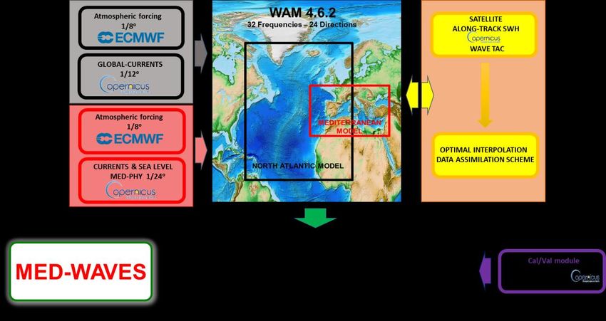
QUID for MED MFC Products Ref: CMEMS-MED-QUID-006-017 MEDSEA_ANALYSISFORECAST_WAV_006_017 Date: 15 January 2020 Issue: 2.0 II PRODUCTION SYSTEM DESCRIPTION II.1 Production centre details PU: HCMR, Greece Production chain: Med-waves External product (2D): spectral significant wave height (Hm0), spectral moments (-1,0) wave period (Tm-10), spectral moments (0,2) wave period (Tm02), wave period at spectral peak / peak period (Tp), mean wave direction from (Mdir), wave principal direction at spectral peak, stokes drift U, stokes drift V, spectral significant wind wave height, spectral moments (0,1) wind wave period, mean wind wave direction from, spectral significant primary swell wave height, spectral moments (0,1) primary swell wave period, mean primary swell wave direction from, spectral significant secondary swell wave height, spectral moments (0,1) secondary swell wave period, mean secondary swell wave direction from. Frequency of model output: 1-hourly analysis and forecast (instantaneous) Geographical coverage: 18.125°W 36.2917°E; 30.1875°N 45.9792°N Horizontal resolution: 1/24° Vertical coverage: Surface Length of forecast: 10 days Frequency of forecast release: Twice per day Analyses: Yes Frequency of analysis release: Twice per day The wave analyses and forecasts for the Mediterranean Sea are produced by the HCMR Production Unit by means of the WAM wave model (described below). The Med-waves system integration is composed of several steps: 1. Upstream Data Acquisition, Pre-Processing and Control of: ECMWF (European Centre for Medium-Range Weather Forecasts) NWP (Numerical Weather Prediction) atmospheric forcing, CMEMS Med MFC and Global MFC currents and CMEMS WAVE TAC SWH satellite NRT observations. 2. Analysis/Forecast: The Med-waves prediction system runs two cycles per day (starting at 00:00 UTC and 12:00 UTC). Each cycle produces 12 hours in the past (analysis) assimilating SWH satellite observations available from the CMEMS WAVE TAC and 10 days (240 hours) into the future (forecast mode). A schematic of the Med-waves operational cycle is shown in Figure 2. 3. Post processing: the model output is processed in order to obtain the products for the CMEMS catalogue. 4. Output delivery. Page 9/ 44
QUID for MED MFC Products Ref: CMEMS-MED-QUID-006-017

 MEDSEA_ANALYSISFORECAST_WAV_006_017 Date: 15 January 2020
 Issue: 2.0

Figure 2: Schematic of the Med-waves production chain at Q2/2021. Each cycle simulates 252 hours:
12 hours in the past (wave analysis) and 240 hours into the future (wave forecasts).

 Page 10/ 44
QUID for MED MFC Products Ref: CMEMS-MED-QUID-006-017

 MEDSEA_ANALYSISFORECAST_WAV_006_017 Date: 15 January 2020
 Issue: 2.0

II.2 Description of the Med-waves modelling system

The wave component of the Mediterranean Forecasting Centre (Med-waves) is providing analyses and
short-term wave forecasts (10 days) for the Mediterranean Sea at 1/24° horizontal resolution.
The Med-waves modelling system consists of a wave model grid implemented over the whole
Mediterranean Sea at 1/24° horizontal resolution nested within a coarser resolution wave model grid
implemented over the Atlantic Ocean (Figure 3).
Med-waves is based on the state-of-the-art third-generation wave model WAM Cycle 4.6.2 which is a
modernized and improved version of the well-known and extensively used WAM Cycle 4 wave model
(WAMDI Group, 1988; Komen et al., 1994), also including different depth scaling (deep – shallow)
allowing for the calculation of the nonlinear wave-wave interactions.
WAM solves the wave transport equation explicitly without any presumption on the shape of the wave
spectrum. Its source terms include the wind input, whitecapping dissipation, nonlinear transfer and
bottom friction. The wind input term is adopted from Snyder et al. (1981). The whitecapping
dissipation term is based on Hasselmann (1974) whitecapping theory. The wind input and
whitecapping dissipation source terms of the present cycle of the wave model are a further
development based on Janssen´s quasi-linear theory of wind-wave generation (Janssen, 1989; Janssen,
1991). The nonlinear transfer term is a parameterization of the exact nonlinear interactions as
proposed by Hasselmann and Hasselmann (1985) and Hasselmann et al., (1985). Lastly, the bottom
friction term is based on the empirical JONSWAP model of Hasselmann et al. (1973).
The Med-waves set-up includes a coarse grid domain with a resolution of 1/6° covering the North
Atlantic Ocean from 75°W to 10°E and from 10°N to 70°N and a nested fine grid domain with a
resolution of 1/24° covering the Mediterranean Sea from 18.125°W to 36.2917°E and from 30.1875°N
to 45.9792°N. The areas covered by the two grids are shown in Figure 3.
The bathymetric map has been constructed using the GEBCO bathymetric data set (GEBCO, 2016) for
the Mediterranean Sea model and the ETOPO2 2-minute data set (NGDC, 2006) for the North Atlantic
model. In both cases mapping on the model grid was done using bi-linear interpolation accompanied
by some degree of isotropic laplacian smoothing.
The Mediterranean Sea model receives full wave spectrum at 3-hourly intervals at its Atlantic Ocean
open boundary from the North Atlantic model. The latter model is considered to have all of its four
boundaries closed assuming no wave energy propagation from the adjacent seas. This assumption is
readily justified for the north and west boundaries of the North Atlantic model considering the
adjacent topography which restricts the development and propagation of swell into the model
domain. The choice of the south boundary location is less obvious and is based on a number of studies
which agree that no important swell energy is expected to propagate northwards from geographical
areas south of 10°N. Specifically, according to Semedo et al. (2011), a swell front present in all seasons
can be identified in the Atlantic Ocean within the latitude band from 15°S (Dec-Jan-Feb) to 15°N (Jun-
Jul-Aug). Young (1999) suggests this swell front never migrates north of the equator. The relatively
narrow geometry of the Atlantic restricts propagation of Southern Ocean swell into the Northern
Hemisphere. According to Alves (2006) storms within the extratropical South Atlantic ocean (below 40
°S) typically propagate to the east spreading swell energy to the Indian Ocean. As for the Atlantic
tropical areas, storms rarely evolve in the south band (between 20°S and the equator) while in the
north tropical band (between the equator and 20°N) summer storms move mostly westwards. During

 Page 11/ 44
QUID for MED MFC Products Ref: CMEMS-MED-QUID-006-017

 MEDSEA_ANALYSISFORECAST_WAV_006_017 Date: 15 January 2020
 Issue: 2.0

winter, the north tropical band can be affected by eastward propagating North Atlantic extratropical
storms generating swells that propagate to the southeast (Alves, 2006).
The wave spectrum is discretized using 32 frequencies, which cover a logarithmically scaled frequency
band from 0.04177 Hz to 0.8018 Hz (covering wave periods ranging from approximately 1 s to 24 s) at
intervals of / = 0.1, and 24 equally spaced directions (15 degrees bin).
The Mediterranean model runs in shallow water mode considering wave refraction due to depth and
currents in addition to depth induced wave breaking. The North Atlantic model runs in deep water
mode with wave refraction due to currents only. The North Atlantic model additionally considers wave
energy damping due to the presence of sea ice. A model grid point is considered to be a sea ice point if
the ice fraction at that point exceeds 60%. At all sea ice points the wave energy is set to zero.

Figure 3: Schematic of the Med-waves system at Q2/2021 (MEDWAM3).

Modifications from default values have been performed in the input source functions. Specifically, the
value of the wave age parameter (zalp) has been set to 0.011 (0.008 is the default) for the
Mediterranean model. In addition, the imposition of a limitation to the high frequency part of the
wave spectrum corresponding to the latest version of the ECMWF wave forecasting system (ECMWF,
2016) has been applied in order to reduce the wave steepness at very high wind speeds.
The system is forced with 10 m above sea surface wind fields obtained from the ECMWF Integrated
Forecasting System (IFS) at 1/8° dissemination resolution, at 3-hourly intervals for the first 90 hours of
the forecast and at 6-hourly intervals from 90 to 240 hours of forecast. Wind is bi-linearly interpolated
onto the model grids. Sea ice coverage fields (daily analysis) are also obtained from ECMWF at the
same horizontal resolution (1/8°) and remain constant during the forecast cycle. With respect to
currents forcing, the Mediterranean Sea model is forced by hourly averaged surface currents and sea
level obtained from CMEMS Med MFC at 1/24° resolution and the North Atlantic model is forced by
daily averaged surface currents obtained from the CMEMS Global MFC at 1/12° resolution. These are
the CMEMS Global and Med MFC surface currents products operational at the time this Med-waves

 Page 12/ 44
QUID for MED MFC Products Ref: CMEMS-MED-QUID-006-017

 MEDSEA_ANALYSISFORECAST_WAV_006_017 Date: 15 January 2020
 Issue: 2.0

system version is released. A schematic of the Med-waves system is shown in Figure 3. Also, Table 3
summarizes the Med-waves modelling characteristics.
Med-waves generates hourly wave fields over the Mediterranean Sea at 1/24° horizontal resolution.
These wave fields correspond either to wave parameters computed by integration of the total wave
spectrum or to wave parameters computed using wave spectrum partitioning. In the latter case the
complex wave spectrum is partitioned into wind sea, primary and secondary swell. Wind sea is defined
as those wave components that are subject to wind forcing while the remaining part of the spectrum is
termed swell. Wave components are considered to be subject to wind forcing when
 ≤ 1.2 × 28 ∗ cos( − )
where is the phase speed of the wave component, ∗ is the friction velocity, is the direction of
wave propagation and is the wind direction. As the swell part of the wave spectrum can be made up
of different swell systems with quite distinct characteristics it is further partitioned into the two most
energetic wave systems, the so called primary and secondary swell. Swell partitioning is done following
the method proposed by Gerling (1992) which finds the lowest energy threshold value at which upper
parts of the spectrum get disconnected with the process repeated until primary and secondary swell is
detected.
The assimilation module
The assimilation system of Med-waves is based on the inherent data assimilation scheme of WAM
Cycle 4.6.2 which consists of performing an optimal interpolation (O.I.) on the along-track SWH
observations retrieved by the altimeters and then re-adjusting the wave spectrum at each grid point
accordingly. This assimilation approach was initially developed by Lionello et al. (1992) and consists of
two steps.
First, a best guess (analysed) field of significant wave height is determined by optimum interpolation
with appropriate assumptions regarding the error covariance matrix. Based on the prejudice that the
wind is the main contributor to the wave model error and that the form of the spectra is essentially
correct, the aim is to obtain the spectrum that the model would have if the correct forcing was used.
One of the key issues of the optimal interpolation approach is the specification of the errors of the
assimilating system. Especially, the specification of the background error covariance matrix, , and the
observation error covariance matrix, , are important since the computation of the gain matrix
depends largely on the structure of these matrices. The Med-waves assimilation module, uses the
default expressions of WAM for the background error covariance matrix

 = ( )

and the observation error covariance matrix
 2
 =
 2
where i and j are, respectively, the model grid points, is the distance from the observation location
to the grid point, is the correlation length, while and stand for the observation and model
errors, respectively. In the above expressions the error is considered as homogeneous and isotropic.
We set the ratio between errors of observations and model (background) equal to 1 and the
correlation length which controls the width of exponential bell equal to 3 deg (~300 km).

 Page 13/ 44
QUID for MED MFC Products Ref: CMEMS-MED-QUID-006-017

 MEDSEA_ANALYSISFORECAST_WAV_006_017 Date: 15 January 2020
 Issue: 2.0

Finally, the weights assigned to the observations are the elements of the gain matrix K:
 = [ + ]−1
where is the observation operator that projects the model solution to the observation location.
The above O.I. analysis procedure applies to significant wave height and 10 m wind speed, U10,
observations that fall within the model domain. For the current version of Med-waves, it has been
applied to altimeter along-track SWH measurements only. No assimilation of U10 measurements is
performed because of a lack of readily available data. It has been shown, through sensitivity testing,
that omitting U10 assimilation in the Mediterranean Sea has negligible effect on output quality.
During the second step, the analysed significant wave height field is used to retrieve the full
dimensional wave spectrum from a first-guess spectrum provided by the model itself, introducing
additional assumptions to transform the information of a single wave height spectrum into separate
corrections for the wind sea and swell components of the spectrum. Two-dimensional wave spectra
are regarded either as wind sea spectra, if the wind sea energy is larger than 3/4 times the total
energy, or, if this condition is not satisfied, as swell. If the first-guess spectrum is mainly wind-sea, the
spectrum is updated using empirical energy growth curves from the model. Additionally, if 10 m winds
observations are available the local forcing wind speed is updated. In case of swell, the spectrum is
updated assuming the average wave steepness provided by the first-guess spectrum is correct but the
wind is not updated. A problem arises when both wind-sea and swell are present. In this situation the
update is done depending on which is the dominant process, which is a limitation of the method.
Prior to assimilation all altimeter SWH observations are subject to quality control procedure. The
primary purpose of the quality control system is to identify observations that are obviously erroneous,
as well as the more difficult process of identifying measurements that fall within valid and reasonable
ranges but nevertheless are erroneous. Accepting this erroneous data can cause an incorrect analysis,
while rejecting extreme, but valid, data can miss important events. The procedure takes into account
thresholds of significant wave height and wind speed (upon availability) observations and root mean
square differences between the model first-guess and the observed SWH.
The wave prediction system runs two cycles per day (starting at 00:00 UTC and 12:00 UTC
respectively). Each cycle is scheduled to simulate 252 hours: 12 hours in the past (analysis) blending
through data assimilation model results with available SWH satellite observations available from
CMEMS WAVE TAC and 10 days (240 hours) into the future (forecast mode). The assimilation step
adopted in this scheme equals to 3 hours. At the end of the analysis mode, a restart file is written that
forms the basis (initial conditions) for the next cycle.
For every day J, the available time series (hourly fields) of the product start from 2 years back, up to
the day J+10. The last ten days of the time series are forecast fields, while the remaining days of the
archive are analysis.

 Page 14/ 44
QUID for MED MFC Products Ref: CMEMS-MED-QUID-006-017

 MEDSEA_ANALYSISFORECAST_WAV_006_017 Date: 15 January 2020
 Issue: 2.0

 North Atlantic
 Mediterranean Sea (Fine)
 (Coarse)
 Model WAM Cycle 4.6.2
 -75oE 10oW -18.125oE 36.291oW
Model Domain
 10oS 70oN 30.1875oN 45.9792oN
 Horizontal
 1/6o x 1/6o 1/24o x 1/24o
 Resolution
 32 (logarithmically spaced)
Frequency Bins
 0.04177-0.80818 Hz
Direction Bins 24 (equally spaced)
 Propagation
 300 s 60 s
 Time-Step
 Forcing 1/8o x 1/8o ECMWF
 (10m winds) operational analysis & 10-days forecasts
 SWH along-track NRT observations
 Data (JASON-3, SENTINEL-3A, SENINTEL-3B,
 assimilation CRYOSAT2, SARAL, CFOSAT, HAIYANG-2B)
 from CMEMS WAVE TAC
 Surface CMEMS GLOBAL MFC CMEMS MED MFC
 Currents (1/12o x 1/12o) (1/24o x 1/24o)
 CMEMS MED MFC
 Sea Level -
 (1/24o x 1/24o)
 Sea Ice 1/8o x 1/8o ECMWF -

Table 3: Med-waves modelling characteristics at Q2/2021

II.3 Upstream data and boundary condition of the WAM model

The CMEMS Med-waves system uses the following upstream data:
 1. Atmospheric forcing: NWP 6-h operational analysis and forecast fields (at 3-hourly intervals for
 the first 90 hours of the forecast and at 6-hourly intervals from 90 to 240 hours of forecast)
 from ECMWF, disseminated at 1/8º horizontal resolution, distributed by the Italian National
 Meteo Service (USAM/CNMA)
 2. Data assimilation: WAVE_GLO_WAV_L3_SWH_NRT_OBSERVATIONS_014_001 inter calibrated
 along track SWH observations from JASON-3, SENTINEL-3A, SENTINEL-3B, SARAL/Altika,
 CRYOSAT-2, CFOSAT and HAIYANG-2B satellite missions, distributed by the CMEMS WAVE TAC
 3. Surface currents forcing: GLOBAL_ANALYSISFORECAST_PHY_001_024 daily averages at 1/12º
 (Atlantic model grid forcing) and MEDSEA_ANALYSISFORECAST_PHY_006_013 hourly averages

 Page 15/ 44
QUID for MED MFC Products Ref: CMEMS-MED-QUID-006-017

 MEDSEA_ANALYSISFORECAST_WAV_006_017 Date: 15 January 2020
 Issue: 2.0

 at 1/24º (Mediterranean model grid forcing) from the CMEMS Global MFC and the CMEMS
 Mediterranean MFC Analysis and Forecast Systems respectively.
4. Sea Level: MEDSEA_ANALYSISFORECAST_PHY_006_013 hourly averages at 1/24º from the
 CMEMS Mediterranean MFC Analysis and Forecast System.
5. Sea-ice cover: daily analysis fields from ECMWF at 1/8º (remain constant during the
 operational cycle) distributed by the Italian National Meteo Service (USAM/CNMA).

 Page 16/ 44
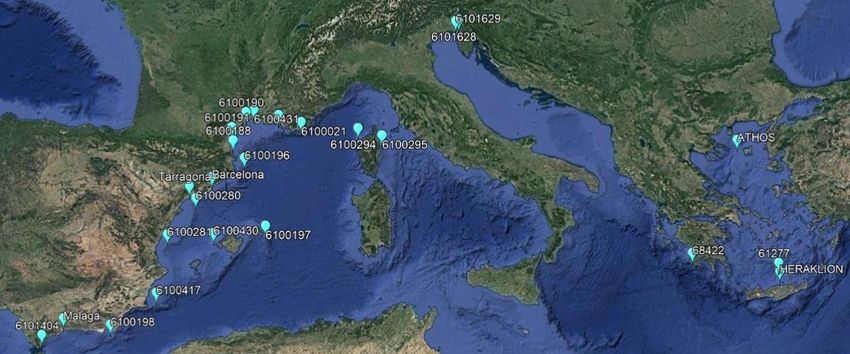
QUID for MED MFC Products Ref: CMEMS-MED-QUID-006-017 MEDSEA_ANALYSISFORECAST_WAV_006_017 Date: 15 January 2020 Issue: 2.0 III VALIDATION FRAMEWORK In order to evaluate and assure the quality of the MEDSEA_ANALYSISFORECAST_WAV_006_017 product of the CMEMS Med-MFC analysis and forecast released in Q2/2021, analysis and first-guess wave parameters were compared to independent and quasi-independent observations respectively over the period of 1 year, July 2019 - July 2020, focusing on model output quality in the Mediterranean Sea. It is noted that all the observations that are assimilated into the system are considered as quasi- independent. In this situation, to assure some level of independency, qualification metrics are calculated before the assimilation of data (i.e. first-guess output). The wave parameters that have been qualified through their comparison with observations include: spectral significant wave height (Hm0) [SWH] spectral moments (0,2) wave period (Tm02) [MWP] The remaining wave parameters included in the CMEMS Med-waves product are not qualified against observational data. This is mainly because there are no relevant observations or because the existing observations are not suited for a robust validation either because of limited data availability or because of data ambiguities (e.g. highly spiky variation). In most of the cases, the quality of these wave parameters is inferred from the quality of those parameters that are thoroughly compared with observations. A valid range, based on climatology and/or expert knowledge, is assigned to each wave parameter. The observations against which modelled wave parameters are compared to include: independent in-situ observations from moored wave buoys obtained from the CMEMS INSITU_MED_NRT_OBSERVATIONS_013_035 dataset, available through the CMEMS In Situ Thematic Assemble Centre (INS-TAC) quasi-independent satellite altimeter observations from the WAVE_GLO_WAV_L3_SWH_NRT_OBSERVATIONS_014_001 dataset, available through the CMEMS WAV-TAC In-situ SWH measurements come from 30 wave buoys in the Mediterranean Sea. Erreur ! Source du renvoi introuvable. depicts their location and unique ID code. MWP measurements were available from 25 of the depicted buoys (see Figure 12). In order to collocate model output and buoy measurements in space, model output was taken at the grid point nearest to the buoy location. In time, buoy measurements within a time window of ± 1 h from model output times at 3-h intervals (0, 3, 6, ..., etc) were averaged. Prior to model-buoy collocation, the in-situ observations were filtered so as to remove those values accompanied by a bad quality flag (Quality Flags included in the data files provided by the INS-TAC). After collocation, visual inspection of the data was carried out, which led to some further filtering of spurious data points. In addition, MWP data below 2 s were omitted from the statistical analysis, since 0.5 Hz (T = 2 s) is a typical cut-off frequency for wave buoys. Metrics have been obtained for individual wave buoys and aggregations of them. In addition to the full Mediterranean Sea domain, the wave buoy groups that have been generated by merging wave buoy observations over regions with similar characteristics are presented in Table 4. Page 17/ 44
QUID for MED MFC Products Ref: CMEMS-MED-QUID-006-017

 MEDSEA_ANALYSISFORECAST_WAV_006_017 Date: 15 January 2020
 Issue: 2.0

Figure 4: Wave buoys locations
Group Name Wave buoys
ES offshore 61198, 61417, 61281, 61280, 61430, 61197, 61196
ES coastal 6101404, Malaga, Tarragona, Barcelona
FR offshore 6100002, 6100001
FR coastal 6100188, 6100191, 6100190, 6100431, 6100290, 6100289
GR Aegean ATHOS, MYKON, 61277, HERAKLION
Table 4: Wave buoy groups: ES = Spanish, FR = French, GR = Greek.

Satellite observations of SWH are from 7 satellite missions: Cryosat-2, SARAL, Jason-3, Sentinel-3a,
Sentinel-3b, CFOSAT, HaiYang2B (H2B). Satellite observations of wind speed, U10, used to validate the
forcing wind fields, come from 5 of these missions (no winds from SARAL and CFOSAT). All satellite
SWH and U10 observations have been cross-calibrated and filtered (Taburet et al., 2019). To collocate
model output and satellite observations the former were interpolated in time and space to the
individual satellite tracks. For each track, corresponding to one satellite pass, along-track pairs of
satellite measurements and interpolated model output were averaged over ~16 km grid cells. This
averaging is intended to break any spatial correlation present in successive 1 Hz (~7 km) observations
and/or in neighbouring model grid output. After collocation, visual inspection of the data was carried
out, which led to some further filtering of spurious data points. In addition, U10 < 2 m/s and SWH < 0.5
m were omitted from the statistical analysis, since a lesser confidence pertains to altimeter
measurements in this range (Rosmorduc et al., 2018). Metrics have been obtained for individual
satellites and aggregations of them, for the full Mediterranean Sea and for the individual sub-regions
defined in Figure 1.
Metrics that are commonly applied to assess numerical model skill and are in alignment with the
recommendations of the EU FP7 project MyWave (A pan-European concerted and integrated approach
to operational wave modelling and forecasting – a complement to GMES MyOcean services, 2012-
2014) have been used to qualify the Med-waves system within the Mediterranean Sea. These include
the RMSD, BIAS, Scatter Index (SI), Pearson Correlation Coefficient (CORR), and the Linear Regression
Slope (LR_SLOPE). The SI, defined here as the standard deviation of model-observation differences
relative to the observed mean, being dimensionless, is more appropriate to evaluate the relative
closeness of the model output to the observations at different locations compared with the RMSD
which is representative of the size of a ‘typical’ model-observation difference. For the same reason,
Relative BIAS and Relative RMSD, i.e. BIAS and RMSD relative to the observed mean, are also used in
the analysis to compare model output quality over different regions and/or time periods. The
LR_SLOPE corresponds to a best-fit line forced through the origins (zero intercept). In addition to the

 Page 18/ 44
QUID for MED MFC Products Ref: CMEMS-MED-QUID-006-017

 MEDSEA_ANALYSISFORECAST_WAV_006_017 Date: 15 January 2020
 Issue: 2.0

aforementioned core metrics, merged Density Scatter and Quantile-Quantile (QQ) plots are provided.
The slope as well as the intercept of a linear regression line is included in these plots. The full set of
metrics used in the qualification of the Med-waves system is defined in Table 5.

 Page 19/ 44
Wave Supporting reference
 Name Description Quantity
 parameter dataset
 Evaluation of Med-waves using independent in-situ observations (Full MED)
 Comparison to wave RMSD, SI, BIAS, CORR, LR_SLOPE between observations
 Spectral significant INSITU_MED_NRT_OBSERV
 SWH-H-CLASS4-MOOR--MED buoy significant wave and analysis, for all Med, for 1-year period and
 wave height (Hm0) ATIONS_013_035
 height seasonally
 Comparison to wave Spectral moments RMSD, SI, BIAS, CORR, LR_SLOPE between observations
 INSITU_MED_NRT_OBSERV
 MWP-H-CLASS4-MOOR--MED buoy mean wave (0,2) wave period and analysis, for all Med, for 1-year period and
 ATIONS_013_035
 period (Tm02) seasonally
 Comparison to wave Merged Quantile-Quantile and Scatter plots between
 SWH-H-CLASS4-MOOR-QQ-MED Spectral significant INSITU_MED_NRT_OBSERV
 buoy significant wave observations and analysis, for all Med, for 1-year
 SWH-H-CLASS4-MOOR-SCATTER-MED wave height (Hm0) ATIONS_013_035
 height period
 Comparison to wave Spectral moments Merged Quantile-Quantile and Scatter plots between
 MWP-H-CLASS4-MOOR-QQ-MED INSITU_MED_NRT_OBSERV
 buoy mean wave (0,2) wave period observations and analysis, for all Med, for 1-year
 MWP-H-CLASS4-MOOR-SCATTER-MED ATIONS_013_035
 period (Tm02) period
 Evaluation of Med-waves using independent in-situ observations (at buoy locations or for wave buoy groups)
 Comparison to wave RMSD, SI, BIAS, CORR, LR_SLOPE between observations
 SWH-H-CLASS2-MOOR-- Spectral significant INSITU_MED_NRT_OBSERV
 buoy significant wave and analysis, for each wave buoy separately, for 1-year
 wave height (Hm0) ATIONS_013_035
 height period
 Comparison to wave Spectral moments RMSD, SI, BIAS, CORR, LR_SLOPE between observations
 MWP-H-CLASS2-MOOR-- INSITU_MED_NRT_OBSERV
 buoy mean wave (0,2) wave period and analysis, for each wave buoy separately, for 1-year
 ATIONS_013_035
 period (Tm02) period
 SWH-H-CLASS2-MOOR-QQ- Spectral significant INSITU_MED_NRT_OBSERV
 buoy significant wave observations and analysis, for each wave buoy
 SWH-H-CLASS2-MOOR-SCATTER- wave height (Hm0) ATIONS_013_035
 height separately, for 1-year period

 MWP-H-CLASS2-MOOR-QQ- INSITU_MED_NRT_OBSERV
 buoy mean wave (0,2) wave period observations and analysis, for each wave buoy
 MWP-H-CLASS2-MOOR-SCATTER- ATIONS_013_035
 period (Tm02) separately, for 1-year period

 Equivalent metrics are produced for individual wave buoy groups (e.g. SWH-H-CLASS4-MOOR-- )

20
QUID for MED MFC Products Ref: CMEMS-MED-QUID-006-017

 MEDSEA_ANALYSISFORECAST_WAV_006_017 Date: 15 January 2020
 Issue: 2.0

 Evaluation of Med-waves using quasi-independent satellite observations (full MED)
 Comparison to WAVE_GLO_WAV_L3_SWH RMSD, SI, BIAS, CORR, LR_SLOPE between observations
 Spectral significant
SWH-H-CLASS4-ALT--MED altimeter significant _NRT_OBSERVATIONS_014 and first-guess, for all Med, for 1-year period and
 wave height (Hm0)
 wave height _001 seasonally
 Comparison to WAVE_GLO_WAV_L3_SWH Merged Quantile-Quantile and Scatter plots between
SWH-H-CLASS4-ALT-QQ-MED Spectral significant
 altimeter significant _NRT_OBSERVATIONS_014 observations and first-guess, for all Med, for 1-year
SWH-H-CLASS4-ALT-SCATTER-MED wave height (Hm0)
 wave height _001 period
Equivalent metrics are produced for individual satellite missions

 Evaluation of Med-waves using quasi-independent satellite observations (MED sub-regions)
 Comparison to WAVE_GLO_WAV_L3_SWH
 Spectral significant RMSD, SI, BIAS, CORR, LR_SLOPE between observations
SWH-H-CLASS4-ALT-- altimeter significant _NRT_OBSERVATIONS_014
 wave height (Hm0) and first-guess, for Med sub-basins, for 1-year period
 wave height _001
 Comparison to WAVE_GLO_WAV_L3_SWH Merged Quantile-Quantile and Scatter plots between
SWH-H-CLASS4-ALT-QQ- Spectral significant
 altimeter significant _NRT_OBSERVATIONS_014 observations and first-guess, for Med sub-basins, for 1-
SWH-H-CLASS4-ALT-SCATTER- wave height (Hm0)
 wave height _001 year period
Equivalent metrics are produced for individual satellite missions

Table 5: List of metrics for Med-waves evaluation using in-situ and satellite observations

 Page 21/ 44
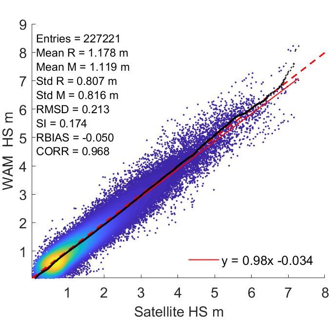
IV VALIDATION RESULTS

IV.1 Significant wave height

Comparison with in-situ observations
Table 6 shows results of the comparison between analysis SWH (model data) and in-situ observations
(reference data), for the Mediterranean Sea as a whole, for the entire year (Jul 2019 - Jul 2020) and
seasonally. In the table, "Entries" refers to the number of model-buoy collocation pairs, i.e. to the
sample size available for the computation of the relevant statistics, R̅ is the mean reference value, M
 ̅ is
the mean model value, STD R and STD M are the standard deviations of the reference and model data
respectively. The remaining quantities are the qualification metrics defined in the previous section.
Erreur ! Source du renvoi introuvable. is the respective merged QQ-Scatter plot for the full 1-year
period. In the figure, the QQ-plot is depicted with black crosses. Also shown are the best fit line with
intercept (red solid line) and the 45° reference line (red dashed line).
 MED ENTRIES ̅ (m)
 R ̅ (m) STD R (m) STD M (m) RMSD (m)
 M SI BIAS (m) CORR LR_SLOPE
 Whole Year 68061 0.88 0.89 0.74 0.74 0.21 0.24 0.01 0.96 1.00
 Winter 16362 1.07 1.08 0.96 0.98 0.26 0.24 0.01 0.97 1.00
 Spring 16738 0.88 0.89 0.68 0.67 0.20 0.22 0.02 0.96 0.99
 Summer 17196 0.66 0.69 0.47 0.49 0.17 0.25 0.02 0.94 1.02
 Autumn 17765 0.92 0.92 0.71 0.71 0.21 0.23 0.00 0.96 0.98

Table 6: Med-waves SWH evaluation against wave buoys' SWH, for the full Mediterranean Sea, for 1
year period and seasonally. Relevant metrics from Table 5: SWH-H-CLASS4-MOOR--MED.

Table 6 shows that the typical difference (RMSD) varies from 0.17 m in summer to 0.26 m in winter.
However, the scatter in summer (0.25) is a little higher than the scatter in winter (0.24) whilst the
lowest correlation coefficient (0.94) is associated with the former season and the highest (0.97) with
the latter. This suggests that the model follows better the observations in winter which is associated
with more well-defined patterns and higher waves than in summer. A similar conclusion has been
derived by other studies (Cavaleri and Sclavo, 2006; Ardhuin et al., 2007; Bertotti et al., 2013) with
respects to wind and wave modelling performance in the Mediterranean Sea. Spring and autumn
present similar statistics with SI values (0.22-0.23) being the best of all seasons and a correlation (0.96)
that is between winter and summer correlation. Small positive BIAS is obtained for all season with the
highest positive value found in summer (4% relative to the observed mean) and the lowest in autumn
(0%). Also, summer has an LR_SLOPE which is above 1, whilst the other seasons have LR_SLOPEs equal
or very close to 1. These values indicate a possible model overestimate which is enhanced in summer.
Indeed, the relevant QQ-Scatter plots (not shown) revealed that the model mostly overestimates the
observations in summer, especially over the higher SWH range. A smaller overestimate, except at very
low waves, was also observed in winter whilst spring and autumn have scatters that are more uniform
along the 45° reference line.

22
QUID for MED MFC Products Ref: CMEMS-MED-QUID-006-017

 MEDSEA_ANALYSISFORECAST_WAV_006_017 Date: 15 January 2020
 Issue: 2.0

Figure 5: QQ-Scatter plots of Med-waves output SWH (Hs) versus wave buoys' observations, for the full
Mediterranean Sea, for 1 year period: QQ-plot (black crosses), 45° reference line (dashed red line),
least-squares best fit line (red line). Relevant metrics from Table 5: SWH-H-CLASS4-MOOR-QQ-MED,
SWH-H-CLASS4-MOOR-SCATTER-MED

Erreur ! Source du renvoi introuvable. depicts the pattern of the agreement between analysis and
observed SWH for different SWH value ranges, for the full Mediterranean Sea. The figure reveals that
the model approximates very well the observations with a small model overestimation of the observed
SWH dominating for waves above about 3 m.
Table 7 shows results of the comparison between analysis SWH and in-situ observations for each of
the wave buoys depicted in Erreur ! Source du renvoi introuvable.. The qualification metrics for the
different buoy locations are also plotted in Erreur ! Source du renvoi introuvable. in order to facilitate
the visualization and interpretation of the relative performance of the wave model at the different
locations. To be able to readily compare the pattern of variation of the different metrics at the
different locations the absolute BIAS and the CORR and LR_SLOPE deviations from unity are plotted in
the bottom plot of Erreur ! Source du renvoi introuvable.. The values of BIAS and LR_SLOPE as given in
Table 7 are shown in the middle plot. For convenience, a map of the wave buoy locations is included in
the figure (top).
Table 7 and Figure 6 reveal that the typical difference (RMSD) at the different buoy locations varies
from 0.13 m to 0.4 m. The Scatter Index (SI) varies from 0.17 at the offshore buoys 6100417 and
6100002, in the western Mediterranean Sea, to 0.41 and 0.53 at the coastal buoys 6101629 and
6101628 respectively in the Gulf of Trieste, in the North Adriatic Sea. In general, SI values above the
mean value for the whole Mediterranean Sea (0.24) are obtained at wave buoys located near the coast
(e.g. coastal Spanish buoys), particularly if these are sheltered by land masses on their north-
northwest (e.g. western French coastline), and/or within enclosed basins characterized by a complex
topography (e.g. ATHOS in the Aegean Sea). As explained in several studies (e.g. Cavaleri and Sclavo,
2006; Bertotti et al., 2013; Zacharioudaki et al., 2015), in these cases, the spatial resolution of the
wave model is often not adequate to resolve the fine bathymetric features whilst the spatial resolution
of the forcing wind model is incapable to reproduce the fine orographic effects, introducing errors to
the wave analysis. The correlation coefficient (CORR) mostly follows the pattern of variation of the SI.
It ranges from 0.78 at buoy 6101628 in the North Adriatic Sea to 0.98 at deep water buoy 6100002,

 Page 23/ 44
QUID for MED MFC Products Ref: CMEMS-MED-QUID-006-017

 MEDSEA_ANALYSISFORECAST_WAV_006_017 Date: 15 January 2020
 Issue: 2.0

offshore from France, and buoy 6100294, west of Corsica, which are well exposed to the prevailing
north-westerly winds in the region. Nevertheless, despite a high correlation, buoy 6100294 has the
largest negative BIAS of -0.18 m whilst the largest positive BIAS of 0.18 m is found at buoy 6100021,
offshore the eastern exit of the Gulf of Lion, France. Both locations are associated with islands and/or
promontories in their vicinity that might not be well resolved by the model. The sign of BIAS varies,
with positive and negative values computed at almost the same number of locations respectively. In
agreement with BIAS, the LR_SLOPE varies between 0.84 at buoy 6100294 to 1.13 at buoy 6100021. In
most of the cases, when BIAS is negative an LR_SLOPE below unity is obtained, pointing to a
prevalence of model underestimation of the observed SWH, and vice versa. Nevertheless, there are
cases when BIAS and LR_SLOPE do not show towards the same direction. This pattern is indicative of a
differential model performance over the different wave height ranges.

 Buoy ID ENTRIES ̅ (m)
 R ̅ (m) STD R (m) STD M (m) RMSD (m)
 M SI BIAS (m) CORR LR_SLOPE
 6101404 2179 0.54 0.53 0.30 0.38 0.18 0.34 -0.01 0.88 1.02
 Malaga 2828 0.46 0.46 0.33 0.36 0.15 0.33 0.00 0.91 0.99
 Tarragona 2920 0.55 0.58 0.39 0.47 0.19 0.34 0.03 0.93 1.08
 Barcelona 2798 0.75 0.69 0.54 0.49 0.17 0.21 -0.07 0.96 0.90
 6100198 2725 1.01 1.10 0.70 0.75 0.23 0.21 0.09 0.96 1.07
 6100417 2935 1.02 1.04 0.68 0.68 0.17 0.17 0.01 0.97 1.00
 6100281 2910 0.83 0.82 0.68 0.68 0.18 0.22 0.00 0.97 0.98
 6100280 2936 0.93 0.94 0.77 0.78 0.20 0.21 0.01 0.97 1.00
 6100430 2916 1.04 1.03 0.82 0.75 0.21 0.20 -0.01 0.97 0.95
 6100197 1899 1.34 1.30 1.07 1.01 0.26 0.19 -0.04 0.97 0.95
 6100196 2924 1.21 1.27 0.98 0.94 0.24 0.20 0.06 0.97 1.00
 61499 2050 0.44 0.44 0.39 0.48 0.16 0.36 0.01 0.96 1.08
 6100002 2900 1.39 1.43 1.01 1.04 0.23 0.17 0.04 0.98 1.02
 6100001 2920 1.04 1.09 0.74 0.84 0.22 0.20 0.05 0.97 1.07
 6100188 2905 0.66 0.64 0.62 0.57 0.18 0.27 -0.03 0.96 0.92
 6100191 2906 0.68 0.70 0.58 0.56 0.17 0.25 0.03 0.96 0.99
 6100190 2897 0.63 0.71 0.56 0.55 0.19 0.27 0.08 0.96 1.04
 6100431 2826 0.71 0.69 0.55 0.50 0.18 0.24 -0.03 0.95 0.93
 6100290 2681 0.72 0.81 0.50 0.54 0.20 0.25 0.09 0.94 1.08
 6100289 2812 0.90 0.88 0.60 0.58 0.19 0.21 -0.02 0.95 0.96
 6100021 1519 1.23 1.40 0.80 0.95 0.40 0.29 0.18 0.93 1.13
 6100294 2361 1.18 1.00 0.96 0.82 0.30 0.21 -0.18 0.98 0.84
 6100295 2496 0.65 0.62 0.51 0.48 0.17 0.25 -0.03 0.95 0.93
 6101628 786 0.25 0.25 0.17 0.21 0.13 0.53 0.01 0.78 1.00
 6101629 911 0.37 0.35 0.27 0.29 0.15 0.41 -0.02 0.85 0.93
 68422 502 0.74 0.77 0.49 0.47 0.15 0.19 0.03 0.96 1.00
 HERAKLION 1854 0.73 0.80 0.57 0.58 0.16 0.20 0.06 0.97 1.05
 61277 2117 1.02 1.06 0.72 0.73 0.20 0.19 0.04 0.96 1.02
 MYKON 2726 1.04 1.14 0.83 0.91 0.25 0.22 0.10 0.97 1.08
 ATHOS 1669 0.77 0.71 0.70 0.64 0.22 0.28 -0.06 0.95 0.90

Table 7: Med-waves SWH evaluation against wave buoys' SWH, for each individual buoy location, for 1
year period. Relevant metrics from Table 5: SWH-H-CLASS2-MOOR--

 Page 24/ 44
QUID for MED MFC Products Ref: CMEMS-MED-QUID-006-017

 MEDSEA_ANALYSISFORECAST_WAV_006_017 Date: 15 January 2020
 Issue: 2.0

Figure 6: SWH metrics (middle, bottom) at buoy locations (top) for 1 year period (plots display metrics
starting from the west and moving eastwards considering a regional arrangement). Bottom plot: CORR
and LR_SLOPE deviations from unity are shown.

 Page 25/ 44
QUID for MED MFC Products Ref: CMEMS-MED-QUID-006-017

 MEDSEA_ANALYSISFORECAST_WAV_006_017 Date: 15 January 2020
 Issue: 2.0

 ES coastal FR coastal GR Aegean

 ES offshore FR offshore

Figure 7: QQ-Scatter plots of Med-waves analysis SWH (Hs) versus wave buoy observations for each of
the wave buoy groups defined in Table 4, for 1 year period: QQ-plot (black crosses), 45° reference line
(dashed red line), least-squares best fit line (red line). Relevant metrics from Table 5: SWH-H-CLASS4-
MOOR-QQ-, SWH-H-CLASS4-MOOR-SCATTER-.

Figure 7 shows QQ-Scatter plots for each of the wave buoy groups defined in Table 4, exhibiting model
performance over the different wave height ranges. It shows that, as expected, the best overall
statistics are obtained for the offshore wave buoy group of France (Relative RMSD = 0.14) which
contains relatively well exposed deep water wave buoys. Nevertheless, a widespread model
overestimation of the observed SWH is seen for heights above about 1 m, which is exacerbated over
the high wave height range. It is noted that this model overestimation is small for buoy 6100002 which
is the most exposed of the two buoys in the group. The behaviour of the model for this group is
expected to be representative of its performance at well-exposed deep water sites. Model
performance is second best (Relative RMSD = 0.16) for the offshore wave buoy group of Spain whose
wave buoys are located closer to the coast compared to the previous group. Here, the QQ-plot crosses
lay close to the reference line and the positive BIAS seems to be mainly due to a small model
overestimation over low wave heights. For waves above about 3 m, a variable pattern of model-
observations agreement is seen with small model underestimation or convergence towards the
observations being the most frequent patterns along the SWH range. Nevertheless, at the wave buoys
located near the Gibraltar Straight (61198, 61417), the model overestimates the observations over
most or all of the SWH range. This is most probably related to a general model overestimation in the
Alboran Sea, as it will be seen later in the comparison with the satellites. Model overestimation
throughout the SWH range is also seen in the Aegean Sea (Relative RMSD = 0.24). This is the case for

 Page 26/ 44
QUID for MED MFC Products Ref: CMEMS-MED-QUID-006-017

 MEDSEA_ANALYSISFORECAST_WAV_006_017 Date: 15 January 2020
 Issue: 2.0

all the individual buoys in the group, especially for those located closer to the coastline, except for
ATHOS where model underestimation is dominant. The poorest model performance is obtained for the
coastal wave buoy groups of France (Relative RMSD = 0.26) and Spain (Relative RMSD = 0.3). For the
coastal wave buoys of France, except for buoy 6100290, the typical scatter distribution is similar to the
one shown for the wave buoy group as a whole. Thus, convergence or small model overestimation of
the observations is seen over the lower SWH range while a small model underestimation is found over
the higher SWH range. At buoy 6100290, which is located near complex topography, a widespread
model overestimation is observed. Generalizing, non-trivial model overestimation of the observed
SWH is not uncommon at wave buoys associated with unresolved bathymetric features in their
surrounding (e.g. 6100021, 61499, 6101628) as also seen in the validation of the Med-waves multi-
year product (Zacharioudaki et al., 2021). Model overestimation of SWH observations above about 0.5-
1 m is also obtained at most of the coastal wave buoys of Spain, as also indicated by the QQ-Scatter
plot of this group. Only at Barcelona buoy, a widespread model underestimation is observed. Model
underestimation is also the dominant mode at buoys 6100294, 6100295 (not included in a group),
located on either side of Corsica island.

 Page 27/ 44
QUID for MED MFC Products Ref: CMEMS-MED-QUID-006-017

 MEDSEA_ANALYSISFORECAST_WAV_006_017 Date: 15 January 2020
 Issue: 2.0

Comparison with satellite observations
This sub-section starts with the comparison of the ECMWF forcing wind speeds, U10, and Med-waves
first-guess SWH, with satellite observations of U10 and SWH respectively, separately for each satellite.
For U10, altimeter observations from CMEMS WAV TAC are available since 2020, therefore, the U10
validation corresponds to a shorter period of about half a year (1 Jan 2020 – 15 Jul 2020) compared to
the SWH validation which spans a full year (16 Jul 2019 – 15 Jul 2020). Figure 8 shows relevant metrics
for the full Mediterranean Sea (top plots) and for the individual sub-regions shown in Figure 1 (bottom
plot).

 U10 SWH

 SWH

Figure 8: (top plots) ECMWF analysis U10 and Med-waves first-guess SWH evaluation against satellite
U10 and SWH respectively, for each satellite, for the full Mediterranean Sea and for the periods Jan
2020 - Jul 2020 and Jul 2019 - Jul 2020 respectively. (bottom plot) As top right plot but for the
individual sub-regions defined in Figure 1. Relevant metrics from Table 5: SWH-CLASS4-ALT--
MED, SWH-H-CLASS4-ALT-- for individual altimeters.

An apparent feature in Figure 8 is a differentiation in model-satellite Relative BIAS found for CFOSAT
with respects to SWH. This is seen for the full Mediterranean Sea and for the individual sub-regions,
especially over the eastern Mediterranean basin. In particular, SWH model-CFOSAT Relative BIAS are
found to be different by 2-4% compared to the values computed for the other model-satellite pairs. In
addition, many spikes have been detected in the CFOSAT dataset. SWH model-H2B comparisons are

 Page 28/ 44
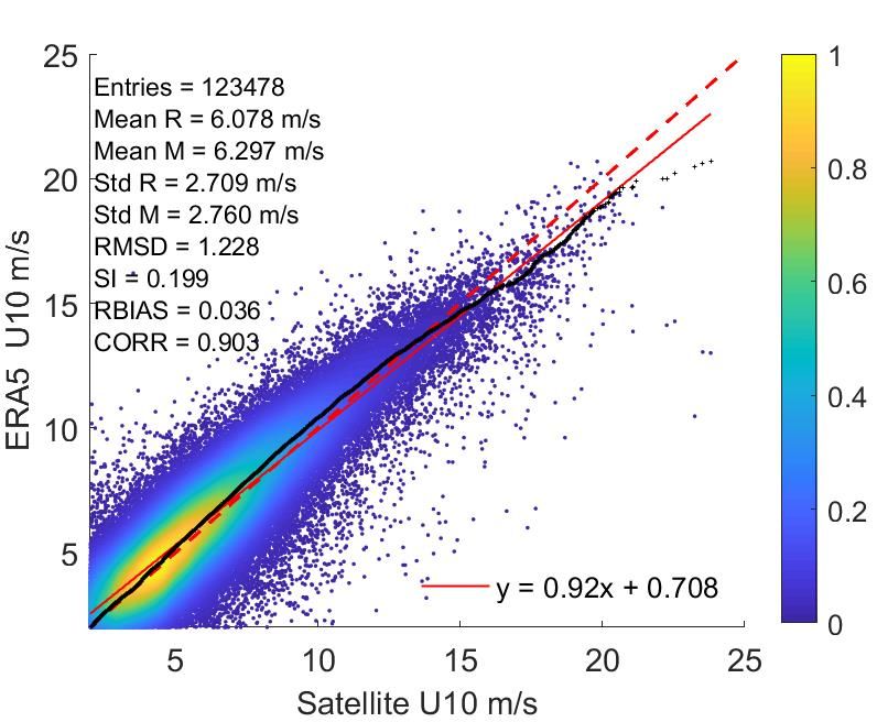
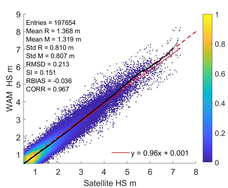
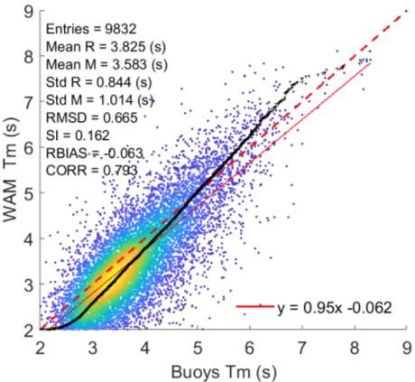
QUID for MED MFC Products Ref: CMEMS-MED-QUID-006-017

 MEDSEA_ANALYSISFORECAST_WAV_006_017 Date: 15 January 2020
 Issue: 2.0

also producing increased negative model BIAS, however, to a lesser degree compared to model-
CFOSAT results. No spikes were found in the H2B dataset. Otherwise, the model-satellite comparison
behaves similarly for the different satellites with the Med-waves model exhibiting its best overall
performance when compared to the observations of SARAL, which are known from literature (e.g.
Sepulveda et al., 2015; Queffeulou et al., 2016) to be of very high quality, better than most satellites.
As a result, in this study, model-SARAL SWH metrics' values are considered as a benchmark and
satellites leading to considerably different results may be excluded from the validation analysis.
Herein, the CFOSAT observations were omitted from the validation because of the numerous spikes in
the dataset and of the increased model BIAS associated with the model-CFOSAT comparisons.
After excluding CFOSAT and merging all other satellite data, Table 8 shows statistics from the
comparison of the Med-waves first-guess SWH and satellite observations of SWH, for the full
Mediterranean Sea, for 1-year period and seasonally. Figure 9 (right) shows the corresponding QQ-
Scatter plot for 1-year period, for the full Mediterranean Sea. Figure 9 (left) shows an equivalent QQ-
Scatter for the ECMWF analysis U10 (Jan 2020 – Jul 2020).

 MED ENTRIES ̅ (m)
 R ̅ (m) STD R (m) STD M (m) RMSD (m)
 M SI BIAS (m) CORR LR_SLOPE
 Whole Year 197654 1.37 1.32 0.81 0.81 0.21 0.15 -0.05 0.97 0.96
 Winter 53847 1.68 1.63 1.03 1.05 0.25 0.14 -0.05 0.97 0.98
 Spring 54434 1.35 1.29 0.73 0.71 0.21 0.15 -0.05 0.96 0.95
 Summer 44513 1.07 1.03 0.49 0.48 0.17 0.15 -0.04 0.94 0.95
 Autumn 44859 1.32 1.27 0.74 0.72 0.21 0.15 -0.05 0.96 0.96
Table 8: Med-waves SWH evaluation against satellite SWH, for the full Mediterranean Sea, for 1 year
period and seasonally. Relevant metrics from Table 5: SWH-H-CLASS4-ALT--MED.

Figure 9 (left) shows that the ECMWF forcing wind model overestimates observed U10 below about 14
m/s and underestimates it above that value. An overall model overestimation of 3.6% (relative to the
observed mean) associated with a linear regression slope of 0.92 have been computed. On the
contrary, Figure 9 (right) shows an overall Med-waves model underestimation of the observed SWH by
3.6% associated with a linear regression slope of 0.96. Nevertheless, in this case the model better
approximates the observations along the SWH range with small model underestimation mainly
observed for SWHs below 4 m. Over high winds and waves, an offset of the wind model negative BIAS
is achieved by the wave model. This result is consistent with previous CMEMS validation activities and
is related to the tuning of the dissipation coefficients in WAM. On the whole, Figure 9 shows that the
performance of Med-waves at offshore locations in the Mediterranean Sea (satellite records near the
coast are mostly filtered out as unreliable) is very good. Comparing to similar results obtained from the
model-buoy comparison (Figure 5), a smaller scatter and a BIAS of different sign is associated with the
model-satellite comparison. SI values are in better agreement at the more exposed waves buoys in the
Mediterranean Sea. At this point, it should be kept in mind that the omission of any SWH < 0.5 m from
the model-satellite comparisons does lead to somewhat improved SI and BIAS values compared to the
values that would have been obtained by including very small waves as is the case for the model-buoy
comparisons (SWH > 0.05 m used).
Table 8 shows the seasonal variation of the Med-waves model performance. The typical difference
with observations (RMSD) varies from 0.17 m in summer to 0.25 m in winter. SI has a very small

 Page 29/ 44
You can also read