Three novel quantum inspired swarm optimization algorithms using different bounded potential fields
←
→
Page content transcription
If your browser does not render page correctly, please read the page content below
www.nature.com/scientificreports
OPEN Three novel quantum‑inspired
swarm optimization algorithms
using different bounded potential
fields
Manuel S. Alvarez‑Alvarado1*, Francisco E. Alban‑Chacón2, Erick A. Lamilla‑Rubio2,
Carlos D. Rodríguez‑Gallegos3 & Washington Velásquez1
Based on the behavior of the quantum particles, it is possible to formulate mathematical expressions
to develop metaheuristic search optimization algorithms. This paper presents three novel quantum-
inspired algorithms, which scenario is a particle swarm that is excited by a Lorentz, Rosen–Morse,
and Coulomb-like square root potential fields, respectively. To show the computational efficacy of
the proposed optimization techniques, the paper presents a comparative study with the classical
particle swarm optimization (PSO), genetic algorithm (GA), and firefly algorithm (FFA). The algorithms
are used to solve 24 benchmark functions that are categorized by unimodal, multimodal, and fixed-
dimension multimodal. As a finding, the algorithm inspired in the Lorentz potential field presents
the most balanced computational performance in terms of exploitation (accuracy and precision),
exploration (convergence speed and acceleration), and simulation time compared to the algorithms
previously mentioned. A deeper analysis reveals that a strong potential field inside a well with weak
asymptotic behavior leads to better exploitation and exploration attributes for unimodal, multimodal,
and fixed-multimodal functions.
Gradient-based and Hessian-based algorithms are widely use in the literature to solve optimization problems
in engineering. This is due to their computational efficiency, which typically require little problem-specific
parameter tuning1. The Gradient-based and Hessian-based algorithms employ iterative process that involves
multivariate scalar function that packages all the information of the partial derivatives of the objective function
(i.e., Gradient function or Hessian matrix) to reach the solution. Some of the most common methods in this
category are: interior point, quasi-Newton, descent gradient, and conjugate gradient1. The main drawback with
such algorithms includes volatility to reach local optima solutions, difficulty in solving discrete optimization
problems, intricacy in the implementation for some complex optimization multivariable problems, and suscep-
tibility to numerical noise2. To tackle the presented deficiencies, some authors suggest the use of metaheuristics
optimization techniques.
In the last two decades, the use of metaheuristics optimization techniques to solve complex, multimodal, high
dimensional and nonlinear engineering problems have become very popular. This is attributed to their simplicity
of implementation, straightforward adaptability to solve optimization problems, and robust search capability to
achieve effective global optima3. Even though there are different metaheuristics optimization techniques, these
can be classified into four main groups as presented in Fig. 1. The first group is called evolutionary algorithm
(EA). The theory behind the EA is based on the evolution in nature. In this field, Genetic Algorithm (GA) emerge
as the most popular. GA was proposed by Holland in 1 9924. GA is inspired by the Darwin evolution t heory4,
in which a population (solution candidates) evolves (best solution) by crossover and mutation processes. In
this way, the solution to the global optima in every iteration (next generation) is assured. Recently, an extensive
recompilation of GA applications can be found in5. Other advanced EAs are Biogeography-Based O ptimizer6,
Clonal Flower P ollination7, Fuzzy Harmony S earch8, Mutated Differential E
volution9, Imperialist Competitive
(2017)10, and Deep Learning with Gradient-based o ptimization11.
1
Faculty of Electrical and Computer Engineering, Escuela Superior Politécnica del Litoral, EC090112 Guayaquil,
Ecuador. 2Faculty of Natural Science and Mathematics, Escuela Superior Politécnica del Litoral,
EC090112 Guayaquil, Ecuador. 3Solar Energy Research Institute of Singapore (SERIS), National University of
Singapore (NUS), Singapore 117574, Singapore. *email: mansalva@espol.edu.ec
Scientific Reports | (2021) 11:11655 | https://doi.org/10.1038/s41598-021-90847-7 1
Vol.:(0123456789)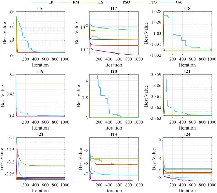
www.nature.com/scientificreports/
Figure 1. Classification of metaheuristics optimization techniques.
The second metaheuristic group corresponds to swarm intelligence (SI). These algorithms incorporate math-
ematical models that describe the motion of a group of creatures in nature (swarms, schools, flocks, and herds)
based on their collective and social behavior. The most well-known SI algorithm presented in the literature is
the Particle Swarm Optimization (PSO), and was proposed by Kennedy and Eberhart in 1 99512. In general, SI
algorithms initialize with multiple particles located in random positions (solution candidates). The particles look
to enhance their position based their position based on their own best positions obtained so far and best particle
of the swarm. The motion process is repeated (iterations) until most of the particle converge to the same position
(best solution). The theory behind SI have been exploited, resulting in novel innovative optimization techniques
(i.e. Dynamic Ant Colony Optimization (2017)13, Bacterial Foraging (2016)14, Fish School Search (2017)15, Moth
Firefly (2016)16, and Chaotic Grey W olf17) for different engineering applications.
The third metaheuristic group is physics-based (PB). Their formulation involves any physical concept used
to describe the behavior through space and time of the matter. PB algorithms can be classified into two main
classes: classical and modern. The term ‘classical’ refers to the optimization techniques that employs classical
physics in their formulations to reach the optima global. In this branch, fits the Greedy Electromagnetism like18,
Improved Central Force19, Multimodal Gravitational Search20, Exponential Big Bang-Big Crunch (BB-BC)21,
and Improved Magnetic Charged System S earch22 algorithms. On the other hand, the term ‘modern’ refers to
the algorithms that employs quantum physics to determine the optima global. Some of the recent algorithms
that fit in this branch are Neural Network Quantum S tates23, Adiabatic Quantum24, and Quantum A nnealing25
optimizations. PB algorithms’ optimization process starts with a random initialization of the matter’s position
(solution candidates). Then, depending on the physical interaction (i.e. kinematic, dynamic, thermodynamic,
hydrodynamic, momentum, energy, electromagnetism, quantum mechanics, etc.) defined in the search space, the
particles improve their position (best solution) and the process is repeated until certain physical rules are satisfied.
The last metaheuristic group is Hybrid algorithm (HA). This group combines the characteristics of the previ-
ous metaheuristics groups to bring new optimization techniques. These algorithms can be classified into four
main groups: EA-SI (i.e. Evolutionary Firefly26), EA-PB (i.e. Harmony Simulated Annealing Search27), SI-PB
(i.e. Big Bang-Big Crunch Swarm O ptimization28) and EA-SI-PB (i.e. Electromagnetism-like Mechanism with
Collective Animal behavior search29). Particularly, the research scope lies on the SI-PB group since it combines
the quantum physics concepts and swarm particle behavior.
The recent literature presents new approaches that use the concepts of quantum mechanics and swarm intel-
ligence for different applications. For instance30, exhibits a Quantum-inspired Glow-worm Swarm Optimisa-
tion (QGSO) to minimize the array style with maximum relative sidelobe level of array (discrete optimization
problem). The algorithm employs the concepts of quantum bits combined with the mathematical behaviour
of social glow-worm swarm to determine the best solution in terms of the position of the best quantum glow-
worm. Authors in31, propose a novel Accelerated Quantum Particle Swarm Optimization (AQPSO) that uses
the concept of quantum mechanics to derive an expression that deals with the position of the quantum particle
trapped in a delta potential well. In order to accelerate the convergence process, the inclusion of an odd number
of observers greater than unity is incorporated to the model. The AQPSO shows high performance resulting in
the application of different power systems application such as optimal placement of static var compensators for
maximum system r eliability31, maximization of savings due to electrical power losses r eduction32, and optimal
maintenance schedule to minimize the operational risk of static synchronous g enerators33 and power g enerators34.
In35–37, quantum ant colony algorithm is used to solve path optimization problems. In this algorithm, every ant
Scientific Reports | (2021) 11:11655 | https://doi.org/10.1038/s41598-021-90847-7 2
Vol:.(1234567890)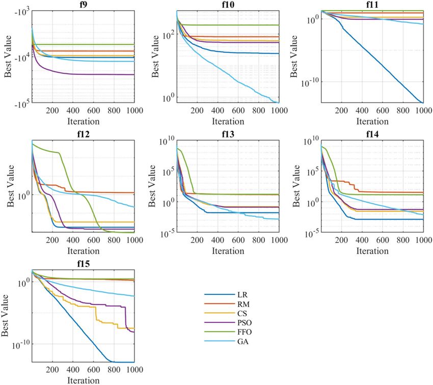
www.nature.com/scientificreports/
Figure 2. Probability density functions associated with the potential fields.
carries a group of quantum bits to represents the position of its own. The ants move according through quantum
rotation gates, which lead to an improvement in their position. As presented, there is plenty of evidence that
demonstrate the computation effective robustness of the quantum SI-PM algorithms. Most of them are driven
by quantum b its30,35–37, and quantum potential w
ells31,38,39. Nevertheless, to the best of our knowledge, there is no
quantum SI-PM in the literature mimicking a quantum particle swarm bounded by Lorentz, Rosen–Morse, and
Coulomb-like Square Root potential fields. This fact encourages the attempt to propose three novel algorithms
and investigate its abilities in solving benchmark optimization problems.
The motivation of this research lies on the No Free Lunch (NFL) theorem, which states that “any two algo-
rithms are equivalent when their performance is averaged across all possible problems”40. The given statement
infers that there is not a best algorithm able to solve any optimization problem. Some algorithms may show effec-
tive performance for a set of problems; however, the same algorithms can result inefficient for a different set of
problems. Therefore, NFL open a pathway to improvement of the existing approaches. Given the foregoing, this
paper proposes three novel hybrid metaheuristics optimization techniques inspired by the movement behaviour
of quantum particle swarm bounded in three different potential fields: Lorentz, Rosen-Morse, and Coulomb-
like Square Root. The given potentials fields are considered due to their simplicity in the analytical solution to
the Schrödinger equation, which are widely studied in the Physics literature41–43. Moreover, these potentials
fields offer certain features that allow to predict the qualitative behaviour of the proposed algorithms in terms
of exploitation and exploration. The base for this statement lies in the probability density function (solution to
the Schrödinger equation), which presents two regime behaviour. The first regime is in between the limits of the
quantum well, while second regime is related to the asymptotic trend at (z → ±∞), as presented in Fig. 2. The
local amplitude of the probability density function (local “height” or probability) represents the strength of the
potential in a region of space. In this sense, the behaviour of the probability density function in between the limits
of the quantum well illustrates the probability of the particle to be near the local attractor that is associated with
the exploration capabilities of the search a lgorithm44. It is important to highlight that the exploration is defined
as the ability of examining a promising area(s) as broadly as possible. By defining a “promising area” as the region
near the local attractor, then more points are expected to be searched in the promising area if more probability
weight is given locally. This means that a higher amplitude (near zero) of the probability density function leads to
a more thoroughly/broadly search in that region, giving rise to more exploration. Hence, the probability density
function that is expected to produce the most exploration in the search algorithm is the Rosen Morse probability
density function, followed by the Lorentz and the Coulomb like Square Root probability density functions. The
behaviour of the probability density function at (z → ±∞) is associated with the global search capabilities of the
algorithm, known in this manuscript as exploitation. Therefore, a slowly decaying probability density function
(weak potential at (z → ±∞)) will be expected to exhibit high exploitation, i.e. further values from the local
attractor will be searched with non-negligible probability44. In this sense it is expected the Lorentz probability
density function to present the best exploitation, followed by the Rosen Morse and the Coulomb-like Square
Root probability density function.
Scientific Reports | (2021) 11:11655 | https://doi.org/10.1038/s41598-021-90847-7 3
Vol.:(0123456789)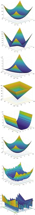
www.nature.com/scientificreports/
Figure 3. QPSO flowchart.
To verify the computational robustness of the proposed approach, several benchmark functions are solved.
Then, the results are compared with the ones obtained by particle swarm optimization, genetic algorithm, and
firefly algorithms. The rest of the paper is organized as follows: “Quantum Particle Swarm Optimization gen-
eral formulation” section presents quantum concepts that describe the scenario of the particle swarm. “Time
independent Schrödinger equation and particle position” section describes the nature of a quantum particle in
a bounded potential field. “Quantum-inspired optimization algorithms” section exhibits the quantum-inspired
proposed optimization algorithms. “Case study” section describe the case study used to test the efficacy of the
proposed algorithms. In “Results” section, the results are analysed and discussed. Finally, “Discussion and con-
clusion” section incorporates the conclusions.
Methodology
Quantum particle swarm optimization general formulation. Quantum particle swarm optimiza-
tion (QPSO) is an advanced heuristic optimization technique that employs the concept of quantum particle
motion to reach the optimal solution. QPSO follows the process described in Fig. 3. The process starts defining
the initial population of the particles SS and total number of iterations MaxIt. The position of the particle (x) rep-
resents a solution candidate to the optimization problem; thus, it can be used to evaluate the objective function.
The next step is to identify the positions called ‘personal best’ and ‘global best’. In this step is relevant to
consider two specific attributes of the particle, which are related to memory and communication. The memory
attribute refers to the ability to save the best position of the particle by comparing its actual position with the
position after the motion. For instance, Fig. 4a shows two scenarios of particle motion. In scenario 1, the particle
has the possibility to move close to the optimum position, therefore, it proceeds to move and saves this posi-
tion as its best position. In scenario 2, the particle has the possibility to move far from the optimum position,
therefore, it will not move and saves its actual position as its best position. The memory attribute is known as
‘personal best’ and denoted by q45,46. The communication attribute refers to the ability to save the particle with
the best position among the swarm. Figure 4b shows a swarm with three particles, resulting in ‘particle 3’ as the
best particle since is the one nearest to the optimum position. The communication attribute is known as ‘global
best’ and is denoted by g45,46.
The process continues with the update of the particles position. For the given purpose, the general mathemati-
cal topology of the swarm intelligence optimization is employed. This is as follows47:
xℓ(k+1) = z xℓ(k) , V + f1 (w1 , u1 ) qℓ(k) − xℓ(k) + f2 (w2 , u2 ) g (k) − xℓ(k) , (1)
Scientific Reports | (2021) 11:11655 | https://doi.org/10.1038/s41598-021-90847-7 4
Vol:.(1234567890)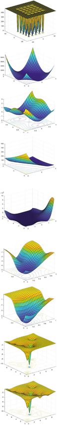
www.nature.com/scientificreports/
(a)
Scenario 1 Scenario 2
Iteration: k Iteration: k
Iteration: k+1 Iteration: k+1
ql ql
Solution space Solution space
Actual position of the particle l Optimum position
Possible position of the particle l ql Personal best
(b) Iteration: k
Solution space
Particle 1 Particle 2 Particle 3
Global best Optimum position
Figure 4. (a) Memory attribute of the particle. (b) Communication attribute of the particle.
(k)
where z represent the displacement of a particle and is a function that depends on xℓ and V, which represent the
actual position x of the particle ℓ at iteration k and the physics phenomena that drives the movement of the par-
ticle, respectively. The functions f1 and f2 correspond to the nature of the swarm intelligence, in which f1 drives
the new position of the particle towards the local optima particle position q, while f2 associates the new position
of the particle with the global optima particle position g. To avoid traps (‘local optima’) that may appear in the
objective function, the authors of the first swarm i ntelligence12 introduced random numbers u and coefficients of
acceleration w such that 0 ≤ w ≤ 2. The suffix ‘1’ and ‘2’ is used to refer to local and global position, respectively.
A simplification of the general formulation of the swarm intelligence optimization, is proposed by authors
in47. The model is based on a trajectory analysis in which the best position of the particle is localized in the search
(k)
space that lies in between the best local and global position. Authors in31 refer to this term as local attractor Dℓ ,
and is used to guide the particle towards a better position. Such model has the f orm47:
(k+1) (k) (k)
xℓ = z(xℓ , V ) + Dℓ ,
(2)
Dℓ(k) = ((r1 u1 )/(r1 u1 + r2 u2 ))qℓ(k) + (1 − (r1 u1 )/(r1 u1 + r2 u2 ))g (k) .
Reference48 presents that for the scenario of a quantum particle trapped in a bounded field, the phenomena
that drives the movement of the particle is given by the relative width a and a function that depends on the
potential well being used, such that48
z xℓ(k) , V = af (V ),
(k) 1
(k)
,
SS (3)
a =
xℓ − qℓ
SS
ℓ=1
where SS is the total number of particles. This last formulation is employed to estimate the new position of the
particle. The function f(V) is analyzed in the following sections of the manuscript.
The last step is to verify the termination criterion using the total number of iterations MaxIt, and convergence
tolerance value ξ . The process finishes if one of the conditions given in Eq. (4) is s atisfied49.
k = MaxIt
Convergence criteria :
SS (k)
ℓ=1 qℓ − SSg (k)
≤ ξ
. (4)
Time independent Schrödinger equation and particle position. QPSO algorithm can be described
through the quantum behaviour of motion of particles. In particular, the case of a particle moving in a bounded
potential field is considered of great interest. Under the given context, particles’ states are depicted by the prob-
ability density function |ψ(�r , t)|2, in the search space r , at time t. The probability density function must s atisfy49.
Scientific Reports | (2021) 11:11655 | https://doi.org/10.1038/s41598-021-90847-7 5
Vol.:(0123456789)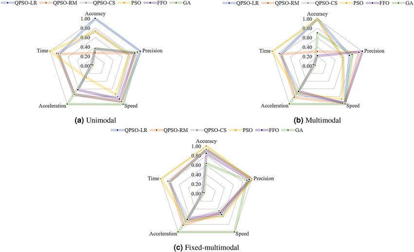
www.nature.com/scientificreports/
+∞
|ψ(�r , t)|2 d�r = 1. (5)
−∞
In order to determine the position of the particle, a measurement is required. For this purpose, a random
number generation simulation is performed u = rand(0, 1). In this sense, the wave function squared must be
normalized with respect to its maximum value, such that
|ψ(�r , t)|2
= u. (6)
max |ψ(�r , t)|2
On the other hand, the time evolution of the wave function ψ( r , t) of a quantum system is generally described
by the Schrödinger e quation49–51:
r , t) = i ∂ ψ(�r , t).
Hψ(� (7)
∂t
The formulation presented in Eq. (7) is also called the time-dependent Schrödinger equation. In this equa-
is the Hamiltonian operator and is the reduced Planck Constant. Nevertheless, for the purpose of this
tion, H
research, a slowly varying process (adiabatic) in which the eigen estate at E = 0 of the particle change accordingly
with the evolution of the potential V is considered. Then, the one-dimension stationary Schrödinger equation
can be used and written as f ollows50,51:
2 ∂ 2
ψ(z) − V (z)ψ(z) = 0. (8)
2m ∂z 2
The last formulation is relevant for the derivation of the term f(V) required in Eq. (3).
Quantum‑inspired optimization algorithms. The following analysis considers wave functions that
belongs to the Hilbert space (ψ(z) ∈ H), that is, the wave function squared |ψ(z)|2 must be normalized with the
boundary condition stablished in Eq. (9)50,51.
lim ψ(z) = 0. (9)
z→±∞
The proposed quantum-inspired optimization algorithms follow the methodology described in Fig. 1. In the
methodology it is required to determine the term f(V), and complete the formulation presented in Eq. (3). In
the following, f(V) is derived for each proposed potential field, which are shown in Fig. 5.
Lorentz potential field (QPSO‑LR). The following algorithm is inspired in the localization of electrons in bonds
formation. This occurs when there is an interaction between electron–donor and electron–acceptor atoms, as
presented in Fig. 5a. The potential field that describes this phenomenon is mathematically described as given in
Eq. (10)52.
2 (2z 2 − a2 )
V (z) = . (10)
2m(z 2 + a2 )2
The displacement of the particle under the Lorentz potential field is obtained by replacing Eq. (10) in Eq.
(8), resulting in Eq. (11).
2 d2 ψ(z) 2 (2z 2 − a2 )
− = 0. (11)
2m dz 2 2m(z 2 + a2 )2 ψ(z)
The solution for the Second Order Linear Ordinary Differential Equation (SLODE) presented in Eq. (11) has
the form given in Eq. (12).
1 3a2 z + z 3
ψ(z) = C1 √ + C2 √ . (12)
a2 + z2 3 a2 + z 2
By applying the boundary condition given in Eq. (9), the result is:
a
C1 = ; C2 = 0. (13)
π
Then,
a
ψ(z) = . (14)
π(a2 + z 2 )
By replacing Eq. (14) in Eq. (6) and solving for z, the result is as follows:
Scientific Reports | (2021) 11:11655 | https://doi.org/10.1038/s41598-021-90847-7 6
Vol:.(1234567890)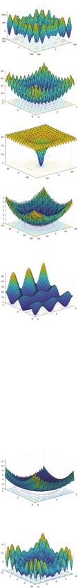
www.nature.com/scientificreports/
(a) interaction
2
Potential field
1
0
-1
-8 -6 -4 -2 0 2 4 6 8
z - displacement
(b)
2
Potential field
1
0
-1
-2
-3 -2 -1 0 1 2 3
z - displacement
(c)
4
Potential field 2
0
-2
-4
-3 -2 -1 0 1 2 3
z - displacement
Figure 5. (a) Lorentz potential field to model donor acceptor interaction. (b) Rosen–Morse potential field to
model molecular vibrations. (c) Coulomb-like square root potential field to model the electron confinement in
graphene.
1−u
z=a . (15)
u
By replacing Eq. (15) in Eq. (3), the conclusion is:
1−u
f (V ) = . (16)
u
Rosen–Morse potential field (QPSO‑RM). The Rosen-Morse potential field can be used to model the vibration
energy spectra produced by the interaction of atoms in a diatomic m olecule53,54, as presented in Fig. 5b. A gen-
eralized form of the Rosen-Morse potential field is given by Eq. (17).
2 tan h2 (z/a) − sec h2 (z/a)
V (z) = . (17)
a2 2m
The displacement of the particle under the Rosen–Morse potential is obtained by replacing Eq. (17) in Eq.
(8), resulting in Eq. (18).
2 d2 ψ(z) 2 tan h2 (z/a) − sec h2 (z/a)
− ψ(Z) = 0. (18)
2m dz 2 2m a2
Using Eq. (9) to normalize the solution to Eq. (18) and solving the SLODE, the result is given by (19).
1
ψ(z) = √ sec h(z/a). (19)
2a
Plugging in Eq. (19) back into Eq. (6) and solving for z, the result is as follows:
√
z = a sec h−1 ( u). (20)
Substituting Eq. (20) in Eq. (3), the conclusion is
Scientific Reports | (2021) 11:11655 | https://doi.org/10.1038/s41598-021-90847-7 7
Vol.:(0123456789)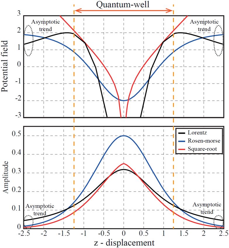
www.nature.com/scientificreports/
√
f (V ) = sec h−1 ( u). (21)
Coulomb‑like square root field (QPSO‑CS). A potential that contains an inverse square root and a linear sym-
metric potential is evaluated. The Coulomb-like square root potential field is commonly employed to model
the electron confinement in g raphene55, as presented in Fig. 5c. Mathematically, the Coulomb-like square root
potential field can be written as given in Eq. (22).
2 0.4 0.6
V (z) = − 3/2 |z|−0.5 + 3 |z| . (22)
2m a a
Similarly, the displacement of the particle under the Coulomb-like Square Root potential is obtained by
replacing Eq. (22) in Eq. (8), which leads to Eq. (23):
2 d2 ψ(z) 2 0.4 −0.5 0.6
− − |z| + |z| ψ(Z) = 0. (23)
2m dz 2 2m a3/2 a3
Using Eq. (9) to normalize the solution to Eq. (23) and solving the SLODE, the result is given by Eq. (24).
1 |z| 3/2
−
ψ(z) = √ e a . (24)
1.69 a
Plugging in Eq. (24) back into Eq. (6) and solving for z, the result is as follows:
2/3
1
z = a ln . (25)
u
Substituting Eq. (25) in Eq. (3), the conclusion is:
2/3
1
f (V ) = ln . (26)
u
The implementation of the proposed optimizations techniques is presented in Algorithm 1. Notice that the
main difference among the proposed algorithms lies in step 11, in which the particle updates its position. This
is because the particle follows a trajectory that mainly depends on the boundary potential field defined in f(V).
Case study. To show the performance of the proposed algorithms (QPSO-LR, QPSO-RM and QPSO-LR),
24 benchmark functions are u sed56. The benchmark functions are categorized by unimodal, multimodal and
fixed-dimension multimodal that are mathematically described in Table 7, 8 and 9, respectively. Unimodal func-
tions are used to analyze the impact of the algorithms when there is one minimum value in a certain interval.
In contrast, multimodal functions are utilized to analyze the algorithms in the presence of several local minima
through the search space. The simulation incorporates for the unimodal and multimodal functions a dimension
(total of variables) of 30, while for fixed-dimension multimodal is as shown in Table 9. Concerning the popula-
Scientific Reports | (2021) 11:11655 | https://doi.org/10.1038/s41598-021-90847-7 8
Vol:.(1234567890)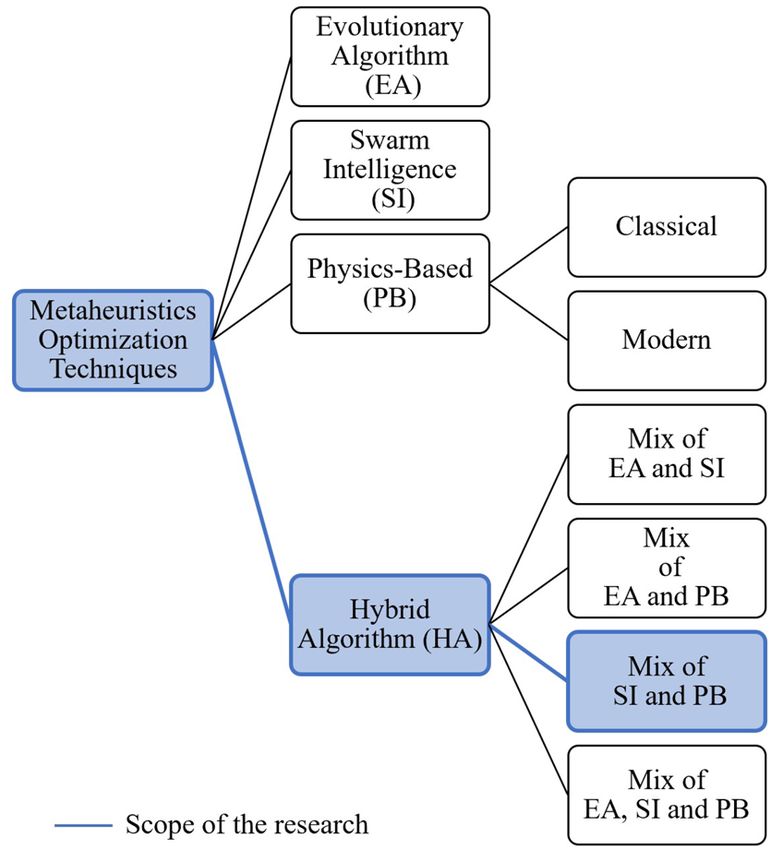
www.nature.com/scientificreports/
Function Metrics QPSO-LR QPSO-RM QPSO-CS PSO FFO GA
δ 4.0379 × 10⁻²⁷ 0.0011 3.1073 × 10⁻³² 5.9653 × 10⁻¹⁹ 4.8991 × 10⁻⁸ 0.1105
f1
φ 1.5526 2.4002 2.0483 1.6922 0.1274 0.6321
δ 4.1492 × 10⁻¹⁹ 0.5925 2.1296 × 10⁻⁷ 2.8087 × 10⁻⁶ 21.6909 0.0685
f2
φ 0.9150 1.1420 2.7324 5.4564 1.6504 0.5758
δ 87.8039 5.4345 × 10³ 123.5104 8.7609 1.2248 × 10³ 2.9055 × 10³
f3
φ 0.4933 0.3378 0.5219 0.7939 0.4788 0.4615
δ 0.0126 31.6220 0.5792 0.4655 26.0576 4.7834
f4
φ 0.5341 0.1802 0.3986 0.4387 0.2965 0.2278
δ 66.0430 668.2517 43.0373 51.0794 188.8109 142.7954
f5
φ 0.9455 0.5255 1.0665 0.8570 1.5627 0.6277
δ 0 866.6000 3.8667 0.2667 9.4000 0.0333
f6
φ 0 0.6728 3.2612 2.9434 0.8686 5.4772
δ 0.0170 0.4136 0.0198 0.0153 0.9466 0.0253
f7
φ 0.4261 0.6762 0.3989 0.6051 0.5203 0.3168
δ 5.5352 6.3865 4.9975 2.8966 11.3206 1.5176
f8
φ 0.2822 0.2962 0.3784 0.6235 0.1053 0.3179
Table 1. Accuracy and precision metrics for unimodal benchmark functions with N = 30, Tmax = 1000 and
Texp = 30.
tion size and total number of iterations, these are 50 and 1000, respectively. To corroborate the significance of the
results, a total of 30 experiments (simulations) are conducted. All the algorithms are tested in MATLAB R2020a
and numerical experiment is set up on Intel Core (TM) i7-6500 Processor, 2.50GHz, 8 GB RAM.
Results
The performance of QPSO-LR, QPSO-RM and QPSO-LR is measured in terms of exploitation (accuracy and
precision), exploration (search speed and acceleration) and simulation time. In addition, to explore the advan-
tages of the proposed algorithms, the same optimization problems are solved using particle swarm optimization
(PSO), genetic algorithm (GA), and firefly optimization (FFO). The results are shown as follows.
Exploitation: accuracy and precision. The exploitation refers to the local search capability around the
promising regions. This can be quantified based on two statistics metrics: accuracy (δ) and precision (φ). The
term accuracy is defined as the absolute value of the difference between the average value and the true value
(reference value) of the quantity being measured, that is, the closeness of the measurements to the true value. On
the other hand, the term precision indicates the closeness of the measurements to each other. The introduced
terms can be mathematically obtained using the true value (xopt ), (x̄)), and standard deviation (σ ) of a set of data,
as given in Eq. (27) and Eq. (28), respectively57.
δ = xopt − x̄ , (27)
φ = |σ/x̄| . (28)
Using the data obtained from the experiments performed with each optimization technique, the mean and
standard deviation can be obtained. Then, by the employment of (27) and (28), the accuracy and the precision
of each optimization technique are obtained. Tables 1, 2 and 3 shows the statistical metrics for unimodal, mul-
timodal, fixed-multimodal benchmark function, accordingly (best values are highlighted in blue). The results
reveal that for each algorithm there is a better match in terms of accuracy and precision depending on the
function. Focusing on the unimodal benchmark functions (f1 − f8 ), QPSO-LR presents the best accuracy for
f1 , f2 , f4 , f6 , f7 , followed by GA in functions f1 , f2 , f6 , f8 and PSO for the functions f4 and f7 . Likewise, if only
precision is considered, there is considerable variation in the algorithms with respect to the functions, e.g., GA
is the most precise for f1 , f2 , f7 , while for f4 and f6 the QPSO-RM and QPSO-LR results to be the most precise,
respectively.
Analyzing the algorithms for the multimodal benchmark functions (f9 − f15 ), there is considerable variation
in accuracy and precision. However, by considering these features separately, the most accurate, but not neces-
sarily the most precise algorithms in descendant order are: QPSO-LR, GA, PSO, FFO, QPSO-CS, QPSO-RM.
In contrast, the algorithms that are more precise, but not necessarily the most accurate in descendant order are:
QPSO-RM, FFO, GA, QPSO-LR, QPSO-CS, and PSO.
For fixed multimodal functions (f16 − f24 ), the results expose that QPSO-LR and QPSO-RM show excellent
results for functions f16 and f19 in terms of accuracy and precision, while PSO responds better to f17 . For the
rest of the functions, all algorithms present acceptable accuracy and precision.
Scientific Reports | (2021) 11:11655 | https://doi.org/10.1038/s41598-021-90847-7 9
Vol.:(0123456789)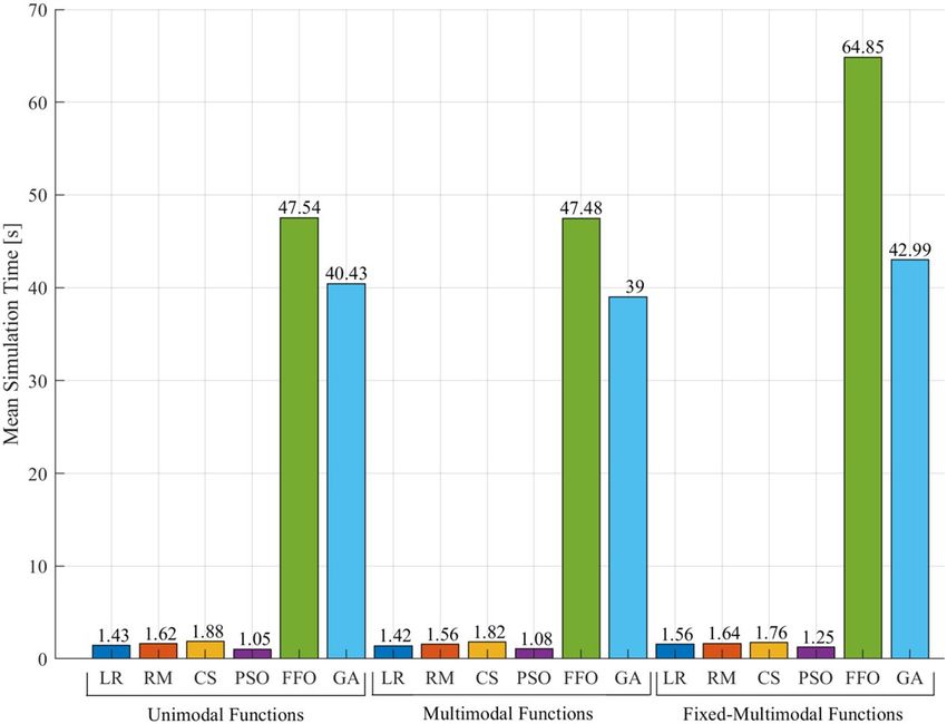
www.nature.com/scientificreports/
Function Metrics QPSO-LR QPSO-RM QPSO-CS PSO FFO GA
δ 1.0377 × 10⁴ 7.5089 × 10³ 9.4712 × 10³ 2.4246 × 10⁴ 5.4177 × 10³ 1.2561 × 10⁴
f9
φ 0.0449 0.0747 0.0598 0.1706 3.4152 × 10⁻¹⁶ 4.6904 × 10⁻⁴
δ 24.1505 82.0155 61.3556 54.1920 193.2863 0.6408
f10
φ 0.3292 0.2662 0.2714 0.2700 0.1876 1.0218
δ 4.0679 × 10⁻¹⁴ 8.6475 1.7671 0.8314 19.9668 0.1446
f11
φ 0.5166 0.1931 0.5818 0.9961 5.5842 × 10⁻¹¹ 0.5556
δ 0.0172 1.2919 0.0330 0.0136 0.0087 0.2078
f12
φ 1.2614 1.1735 1.3155 1.2714 1.3300 0.4605
δ 0.0173 14.5092 0.1630 0.1349 16.5333 0.0016
f13
φ 2.2743 0.5130 2.0342 1.9827 0.4402 3.6775
δ 0.0015 33.5424 0.0288 0.0569 13.9971 0.0082
f14
φ 2.5931 0.3051 4.2382 5.1166 1.3473 1.1503
δ 1.1676 × 10⁻¹³ 1.7340 3.4012 × 10⁻⁸ 7.2088 × 10⁻⁹ 2.8835 0.0047
f15
φ 1.0440 0.9820 4.9304 2.8034 0.5131 0.3573
Table 2. Accuracy and precision metrics for multimodal benchmark functions with N = 30, Tmax = 1000 and
Texp = 30.
Function Metrics QPSO-LR QPSO-RM QPSO-CS PSO FFO GA
δ 0.6460 0.6624 0.5710 0.5531 0.4058 0.4688
f16
φ 0.2617 0.2410 0.2592 0.2439 0.3711 0.4651
δ 0.0023 0.0011 0.0023 2.2142 × 10⁻⁴ 0.0060 0.0067
f17
φ 2.3522 2.5454 2.3449 0.6455 1.9599 1.3437
δ 1.5465 × 10⁻⁶ 1.5465 × 10⁻⁶ 1.5465 × 10⁻⁶ 1.5465 × 10⁻⁶ 1.5465 × 10⁻⁶ 1.3332 × 10⁻⁴
f18
φ 6.4438 × 10⁻¹⁶ 6.3831 × 10⁻¹⁶ 6.5062 × 10⁻¹⁶ 6.5675 × 10⁻¹⁶ 1.813 × 10⁻¹⁵ 4.0007 × 10⁻⁴
δ 1.1264 × 10⁻⁴ 1.1264 × 10⁻⁴ 1.1264 × 10⁻⁴ 1.1264 × 10⁻⁴ 0.0768 0.0011
f19
φ 0 0 0 0 0.8873 0.0066
δ 7.9491 × 10⁻¹⁴ 7.7272 × 10⁻¹⁴ 7.9491 × 10⁻¹⁴ 7.8601 × 10⁻¹⁴ 1.5986 × 10⁻¹⁴ 0.0083
f20
φ 4.6649 × 10⁻¹⁶ 3.7488 × 10⁻¹⁶ 5.2010 × 10⁻¹⁶ 1.8436 × 10⁻¹⁶ 8.7753 × 10⁻¹⁵ 0.0087
δ 1.7852 × 10⁻⁵ 1.7852 × 10⁻⁵ 1.7852 × 10⁻⁵ 1.7852 × 10⁻⁵ 1.7852 × 10⁻⁵ 5.0918 × 10⁻⁵
f21
φ 7.0163 × 10⁻¹⁶ 6.9801 × 10⁻¹⁶ 7.0159 × 10⁻¹⁶ 7.0159 × 10⁻¹⁶ 3.9481 × 10⁻¹⁶ 1.8331 × 10⁻⁵
δ 0.0495 0.0456 0.0535 0.0535 0.1030 0.0496
f22
φ 0.0183 0.0181 0.0185 0.0185 0.0131 0.0183
δ 3.3818 4.2363 4.2274 2.6751 4.7546 3.2649
f23
φ 0.4677 0.5803 0.5433 0.4643 0.5808 0.4994
δ 4.5851 3.8040 3.5104 1.3978 4.7708 2.2613
f24
φ 0.6081 0.5526 0.5492 0.3164 0.6589 0.4241
Table 3. Accuracy and precision metrics for fixed-multimodal benchmark functions with Tmax = 1000 and
Texp = 30.
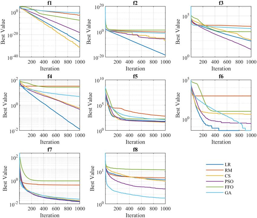
Exploration: speed and acceleration. The exploration is defined as the ability of examining the promis-
ing area(s) of the search space as broadly as possible56. The exploration is closed related with the convergence
behaviour, which is shown in Figs. 6, 7 and 8. These graphs represent the evolution of the best solution through
every iteration performed. It can be appreciated that depending on the type of function on which the algorithms
are applied, presents certain patterns. For instance, functions f1 , f2 , f3 , f4 , f5 (independently of the employed
algorithm) present a linear convergence behaviour, while for the rest of functions the behaviour is exponential.
To quantify the exploration, the average search speed and acceleration of each algorithm is calculated using
the Allan v ariances58. The first Allan variance index measures search speed, i.e. the distance variation of best
search agent C in every iteration k, which is mathematically described in Eq. (29). The second Allan variation
index measures the search acceleration, i.e. the search speed variation, which is mathematically described in
Eq. (30).
kmax C(k + 1) − C(k)
k=1
ω = , (29)
�k
Scientific Reports | (2021) 11:11655 | https://doi.org/10.1038/s41598-021-90847-7 10
Vol:.(1234567890)www.nature.com/scientificreports/
Figure 6. Convergence behaviour of the unimodal benchmark functions.
kmax ω(k + 1) − ω(k)
α = k=1 . (30)
�k
Tables 4, 5 and 6 shows the search speed and acceleration for each optimization technique grouped by uni-
modal, multimodal, and fixed multimodal functions, respectively (best values are highlighted in blue). For all
types of functions, GA algorithm exhibits the highest degree of average search speed and acceleration. However,
speed and acceleration attributes does not assure good precision, accuracy, or simulation time. Therefore, a more
scrutiny analysis is required to develop a proper comparison between optimization methods, as presented in
the next sections.
Simulation time. Another important aspect to evaluate is the simulation time performance. Figure 9
shows the average execution time for each optimization algorithm. The results reveal that FFO and GA present
higher time simulation (exceeds in approximately between 34 to 48 times) compared with the rest of the optimi-
zation techniques. Therefore, QPSO-LR, QPSO-RM, QPSO-CS and PSO present better performance in terms of
simulation time than FFO and GA.
Overall performance. The performance in terms of accuracy, precision, search speed, search acceleration,
and simulation time of each optimization technique is quantitative defined by the grade rules presented in (31)
to (35), respectively. These rules are developed to facilitate the comparison between optimization techniques
under the following criterion: ‘+ 3’ excellent performance, ‘+ 2’ good performance, ‘+ 1’ fair performance, ‘+ 0’
low performance. Once the values are assigned, the average of the function by groups (unimodal, multimodal,
fixed multimodal) is taken. Then, the values are normalized based on the highest average.
+3 if δ < 1 × 10⁻⁶
+2 if 1 × 10⁻⁶ ≤ δ < 1 × 10⁻³
ruleδ = −3 , (31)
+1 if 1 × 10 ≤ δ < 1
0 if δ ≥ 1
Scientific Reports | (2021) 11:11655 | https://doi.org/10.1038/s41598-021-90847-7 11
Vol.:(0123456789)www.nature.com/scientificreports/
Figure 7. Convergence behaviour of the multimodal benchmark functions.
+3 if σ < 1 × 10⁻³
ruleσ = +2 if 1 × 10⁻³ ≤ σ < 1 ,
(32)
+1
if 1≤σ 1 × 10⁶
+2 if 1 × 10³ < ω ≤ 1 × 10⁶
ruleω = 1 , (33)
+1 if 1 < ω ≤ 1 × 10³
0 if ω≤3
+3 if α > 1000
+2 if 100 < α ≤ 1000
ruleα = 1 , (34)
+1
if 1 < α ≤ 100
0 if α≤1
+3 if τwww.nature.com/scientificreports/
Figure 8. Convergence behaviour of the fixed-multimodal benchmark functions.
Function Metrics QPSO-LR QPSO-RM QPSO-CS PSO FFO GA
ω 1.4443 × 10³ 1.5990 × 10³ 1.7382 × 10³ 5.9047 × 10² 4.7911 × 10² 3.3144 × 10³
f1
α 3.4075 × 10² 4.2430 × 10² 3.3948 × 10² 6.0829 5.2972 2.0046 × 10³
ω 4.1564 × 10⁷ 7.1210 × 10⁷ 3.8718 × 10² 5.1176 × 10² 5.1176 × 10¹⁰ 1.1566 × 10¹⁸
f2
α 4.2608 × 10⁷ 7.2078 × 10⁷ 7.6250 × 10⁸ 6.3001 × 10⁻² 3.6744 × 10¹⁰ 1.1979 × 10¹⁸
ω 2.2971 × 10³ 2.6881 × 10³ 2.3607 × 10³ 9.8210 × 10² 1.7612 × 10³ 4.7806 × 10⁴
f3
α 3.3765 × 10² 5.8023 × 10² 5.2257 × 10² 51.6621 1.4315 × 10² 4.6678 × 10⁴
ω 1.5963 1.5752 1.0108 0.7047 0.4801 2.3429
f4
α 0.1307 0.1186 0.0329 0.0237 0.0132 0.8982
ω 4.4969 × 10⁶ 4.7306 × 10⁶ 6.3133 × 10⁶ 1.0640 × 10⁶ 7.5646 × 10⁶ 1.6173 × 10⁷
f5
α 1.9421 × 10⁶ 1.6195 × 10⁶ 1.4387 × 10⁶ 6.5665 × 10² 2.0199 × 10⁵ 1.3257 × 10⁷
ω 1.5644 × 10³ 1.5276 × 10³ 1.7360 × 10³ 5.9708 × 10² 4.7453 × 10² 3.0891 × 10³
f6
α 4.8047 × 10² 3.8717 × 10² 2.9077 × 10² 9.3619 9.2238 1.8074 × 10³
ω 2.1368 2.3284 3.0930 0.4842 3.2862 7.9698
f7
α 0.7444 0.8915 0.6685 0.0040 0.0829 6.5391
ω 0.34833 0.4149 0.3111 0.1649 0.3147 1.1468
f8
α 0.0707 0.0842 0.0743 0.0041 0.0278 0.6206
Table 4. Convergence speed and acceleration metrics for unimodal benchmark functions with N = 30, Tmax
= 1000 and Texp = 30.
Scientific Reports | (2021) 11:11655 | https://doi.org/10.1038/s41598-021-90847-7 13
Vol.:(0123456789)www.nature.com/scientificreports/
Function Metrics QPSO-LR QPSO-RM QPSO-CS PSO FFO GA
ω 1.4137 × 10² 1.4873 × 10² 1.3877 × 10² 2.6002 × 10² 90.5291 1.8003 × 10²
f9
α 6.0517 6.7619 0.8768 28.8637 80.4336 90.3119
ω 7.1803 9.1616 6.6542 2.4200 7.2001 14.7343
f10
α 0.6570 1.1580 0.7452 0.0361 0.4907 6.6963
ω 0.3426 0.3647 0.3127 0.2036 0.0001 0.0516
f11
α 0.0116 0.0167 1.688 × 10⁻⁴ 0.0045 0.0001 19.2122
ω 12.9950 14.1370 15.6384 5.2224 4.3928 30.8202
f12
α 2.9750 3.7139 2.5028 0.0400 0.0820 19.2122
ω 1.0457 × 10⁷ 8.9922 × 10⁶ 1.3693 × 10⁷ 1.2975 × 10⁶ 9.9214 × 10⁶ 4.5856 × 10⁷
f13
α 4.6454 × 10⁶ 4.2749 × 10⁶ 3.1766 × 10⁶ 2.7464 × 10³ 2.8049 × 10⁵ 4.1327 × 10⁷
ω 1.9438 × 10⁷ 1.9614 × 10⁷ 2.7256 × 10⁷ 3.4698 × 10⁶ 1.6631 × 10⁷ 7.3698 × 10⁷
f14
α 7.4400 × 10⁶ 8.2036 × 10⁶ 7.1400 × 10⁶ 1.3277 × 10⁴ 5.1217 × 10⁵ 6.1365 × 10⁷
ω 1.4280 1.6201 1.3598 0.5925 1.3838 2.7137
f15
α 0.2589 0.1861 0.0947 0.0103 0.0773 1.2823
Table 5. Accuracy and precision metrics for multimodal benchmark functions with N = 30, Tmax = 1000 and
Texp = 30.
Function Metrics QPSO-LR QPSO-RM QPSO-CS PSO FFO GA
ω 17.1710 17.1800 17.1860 17.1130 17.1860 6.2410
f16
α 0.5586 0.0081 0.0088 0.0802 0.0080 0.2768
ω 0.0014 0.0019 0.0020 0.0013 0.0030 1.8499 × 10²
f17
α 0.0008 0.0012 0.0012 0.0007 0.0011 1.9159 × 10²
ω 0.0090 0.0128 0.0155 0.0005 0.0151 32.3928
f18
α 0.0062 0.0086 0.0109 0.0019 0.0070 33.5288
ω 0.0186 0.0241 0.0200 0.0114 0.0306 1.9380
f19
α 0.0107 0.0173 0.0130 0.0042 0.0007 1.9688
ω 0.3086 0.5306 0.4182 0.3813 0.2147 3.1195 × 10³
f20
α 0.1404 0.3354 0.2157 0.2384 0.1398 3.2301 × 10³
ω 0.0040 0.0067 0.0057 0.0036 0.0032 0.1029
f21
α 0.0025 0.0041 0.0032 0.0012 0.0022 0.0998
ω 0.0351 0.0338 0.0323 0.0215 0.0217 0.1005
f22
α 0.0168 0.0112 0.0132 0.0064 0.0064 0.0702
ω 0.1875 0.1610 0.1512 0.1948 0.1671 0.1919
f23
α 0.0469 0.0178 0.0193 0.0058 0.0018 0.0337
ω 0.1552 0.1682 0.1937 0.1922 0.1640 0.1606
f24
α 0.0174 0.0156 0.0200 0.0060 0.0025 0.0329
Table 6. Accuracy and precision metrics for fixed-multimodal benchmark functions with N = 30, Tmax =
1000 and Texp = 30.
As a general trend, it can be seen in Fig. 10 that for the three types of functions the algorithm that is closest
on average to 100% performance in all five indexes is the QPSO- LR, followed by the PSO, the QPSO- CS and
finally the GA and FFA method. A closer examination reveals:
• With respect to accuracy, the QPSO-LR, PSO and QPSO-CS go first, second and third respectively with an
average performance of 97%, 91% and 88%.
• In terms of precision the FFO, the QPSO-LR and GA can be ranked as first, second and third, respectively
with an average performance over the three type of functions of 94%, 91%, and 87%.
• Referring to speed of convergence, GA technique can be ranked first with 100% average performance, fol-
lowed by the QPSO-LR, 83% and the QPSO-RM, 80%.
• In terms of acceleration of convergence GA has 100%, followed by QPSO-RM and QPSO-LR with 80% and
74% of average performance, respectively.
• Regarding the simulation time, PSO can be ranked at the top with an average performance of 100% being
followed by the QPSO-CS, QPSO-RM and the QPSO-LR with an average performance between 85% and
80%.
Scientific Reports | (2021) 11:11655 | https://doi.org/10.1038/s41598-021-90847-7 14
Vol:.(1234567890)www.nature.com/scientificreports/
Figure 9. Average simulation time.
Figure 10. Optimization techniques performance categorized by type of function.
To get a better understanding of the performance in terms of exploitation, the accuracy and precision are aver-
aged for each type of function (Unimodal, Multimodal and Fixed multimodal). The same process is done with
search speed and acceleration to quantify exploration (see Table 10). As a result, the exploitation performance
of QPSO-LR is ranked first, followed by the QPSO-RM and the QPSO-CS (just considering the proposed
approaches). This is expected since the Lorentz potential field is the weakest as (z → ±∞) and the Coulomb
like potential diverges as (z → ±∞), being the strongest. Regarding exploration the QPSO-RM is ranked first,
Scientific Reports | (2021) 11:11655 | https://doi.org/10.1038/s41598-021-90847-7 15
Vol.:(0123456789)www.nature.com/scientificreports/
followed by the QPSO-LR and the QPSO-CS. Again, this is also expected since the Rosen Morse potential field
is the strongest in between the limits of the quantum well and the Coulomb like potential diverges towards −∞,
being the weakest (steepest too).
An increase in exploration and a slightly decrease in exploitation is observed in the multimodal functions
compared to the unimodal, due to the high number of traps that may exist in the hypersurface being searched.
Also, an increase in exploitation and decrease in exploration are observed in the fixed multimodal functions
compared to unimodal, attributed to irregular hypersurface formed. While the behaviour of the search algorithm
may change for each type of function, the QPSO-LR always exhibited higher exploitation and moderate-high
exploration. Being the combination of weak potential at (z → ±∞) and moderate steepness between the limits
of the quantum well that are responsible of such trend.
Discussion and conclusion
Three novel quantum-behaved swarm optimization algorithms based on Lorentz (QPSO-LR), Rosen–Morse
(QPSO-RM) and Coulomb-like Square Root (QPSO-CS) potential fields are proposed. The QPSO-LR, QPSO-
RM, and QPSO-CS are inspired in the models of donor acceptor interaction between particles, molecular vibra-
tions, and electron confinement in graphene, respectively.
To verify the efficacy of the proposed optimization techniques, twenty-four test functions grouped by uni-
modal, multimodal, fixed multimodal are employed to benchmark their performance in terms of exploration
(accuracy and precision), exploitation (search speed and acceleration), and simulation time. The results show
that the proposed approaches (QPSO-LR, QPSO-RM, and QPSO-CS) present several advantages in compari-
son to traditional optimization techniques, such as, PSO, FFO, and GA. For instance, QPSO-LR exhibits better
accuracy performance than PSO, FFA, and GA, for all the type functions; QPSO-CS shows better precision than
GA and PSO in overall; QPSO-RM and QPSO-LR have a faster speed and acceleration of search than PSO and
FFO; QPSO-LR, QPSO-RM, and QPSO-CS show significant computation time performance than FFO and GA.
Among the proposed optimizations techniques, there is not one that show the best performance in all the
given attributes (exploration, exploitation, and simulation time), however, QPSO-LR is the most balanced, which
makes it a powerful global searcher for different applications. Therefore, the aim of future research is to investigate
the use of QPSO-LR combined with other computational intelligence methodologies, such as fuzzy systems and
neural networks for optimization in multivariable processes in order to enhance the performance of the approach.
Case study: benchmark functions
See Tables 7, 8 and 9.
Scientific Reports | (2021) 11:11655 | https://doi.org/10.1038/s41598-021-90847-7 16
Vol:.(1234567890)www.nature.com/scientificreports/
Table 7. Unimodal benchmark functions.
Scientific Reports | (2021) 11:11655 | https://doi.org/10.1038/s41598-021-90847-7 17
Vol.:(0123456789)www.nature.com/scientificreports/
Table 8. Multimodal benchmark functions.
Scientific Reports | (2021) 11:11655 | https://doi.org/10.1038/s41598-021-90847-7 18
Vol:.(1234567890)www.nature.com/scientificreports/
Table 9. Fixed-dimension multimodal benchmark functions.
Overall performance of exploitation and exploration of the proposed approaches
See Table 10.
Scientific Reports | (2021) 11:11655 | https://doi.org/10.1038/s41598-021-90847-7 19
Vol.:(0123456789)www.nature.com/scientificreports/
Function type Search algorithm Exploitation Exploration
QPSO-LR 1.00 0.84
Unimodal QPSO-CS 0.60 0.74
QPSO-RM 0.60 0.84
QPSO-LR 0.86 0.86
Multimodal QPSO-CS 0.60 0.83
QPSO-RM 0.62 0.90
QPSO-LR 0.96 0.64
Fixed multimodal QPSO-CS 0.90 0.60
QPSO-RM 0.96 0.66
Table 10. Exploitation and exploration performance.
Received: 3 March 2021; Accepted: 18 May 2021
References
1. Venter, G. Review of optimization techniques. In Encyclopedia of Aerospace Engineering (ed. Venter, G.) (Wiley, 2010).
2. Shrestha, A. & Mahmood, A. Review of deep learning algorithms and architectures. IEEE Access 7, 53040–53065 (2019).
3. Hussain, K., Salleh, M. N. M., Cheng, S. & Shi, Y. Metaheuristic research: A comprehensive survey. Artif. Intell. Rev. 52, 2191–2233
(2019).
4. Chambers, L. D. Practical Handbook of Genetic Algorithms: Complex Coding Systems, Vol. 3 (CRC Press, 2019).
5. Saini, N. Review of selection methods in genetic algorithms. Int. J. Eng. Comput. Sci. 6, 22261–22263 (2017).
6. Simon, D. Biogeography-based optimization. IEEE Trans. Evol. Comput. 12, 702–713 (2008).
7. Sayed, S.A.-F., Nabil, E. & Badr, A. A binary clonal flower pollination algorithm for feature selection. Pattern Recogn. Lett. 77,
21–27 (2016).
8. Pandiarajan, K. & Babulal, C. Fuzzy harmony search algorithm based optimal power flow for power system security enhancement.
Int. J. Electr. Power Energy Syst. 78, 72–79 (2016).
9. Cui, L., Li, G., Lin, Q., Chen, J. & Lu, N. Adaptive differential evolution algorithm with novel mutation strategies in multiple sub-
populations. Comput. Oper. Res. 67, 155–173 (2016).
10. Xu, S., Wang, Y. & Lu, P. Improved imperialist competitive algorithm with mutation operator for continuous optimization problems.
Neural Comput. Appl. 28, 1667–1682 (2017).
11. Dalgaard, M., Motzoi, F., Sørensen, J. J. & Sherson, J. Global optimization of quantum dynamics with alphazero deep exploration.
npj Quantum Inf. 6, 1–9 (2020).
12. Kennedy, J. & Eberhart, R. Particle swarm optimization. In Proc. ICNN’95-International Conference on Neural Networks, Vol. 4,
1942–1948 (IEEE, 1995).
13. Olivas, F. et al. Ant colony optimization with dynamic parameter adaptation based on interval type-2 fuzzy logic systems. Appl.
Soft Comput. 53, 74–87 (2017).
14. Devabalaji, K. & Ravi, K. Optimal size and siting of multiple dg and dstatcom in radial distribution system using bacterial foraging
optimization algorithm. Ain Shams Eng. J. 7, 959–971 (2016).
15. de Albuquerque, I. M. C., Neto, F. B. D. L. et al. Fish school search algorithm for constrained optimization. Preprint at http://a rXiv.
org/1707.06169 (2017).
16. Zhang, L., Mistry, K., Neoh, S. C. & Lim, C. P. Intelligent facial emotion recognition using moth-firefly optimization. Knowl.-Based
Syst. 111, 248–267 (2016).
17. Kohli, M. & Arora, S. Chaotic grey wolf optimization algorithm for constrained optimization problems. J. Comput. Des. Eng. 5,
458–472 (2018).
18. Zeng, Y., Zhang, Z., Kusiak, A., Tang, F. & Wei, X. Optimizing wastewater pumping system with data-driven models and a greedy
electromagnetism-like algorithm. Stoch. Environ. Res. Risk Assess. 30, 1263–1275 (2016).
19. Liu, J. & Wang, Y.-P. An improved central force optimization based on simplex method. J. Zhejiang Univ. (Eng. Sci.) 48, 2 (2014).
20. Yazdani, S., Nezamabadi-pour, H. & Kamyab, S. A gravitational search algorithm for multimodal optimization. Swarm Evol.
Comput. 14, 1–14 (2014).
21. Hasançebi, O. & Azad, S. K. An exponential big bang-big crunch algorithm for discrete design optimization of steel frames. Comput.
Struct. 110, 167–179 (2012).
22. Kaveh, A., Mirzaei, B. & Jafarvand, A. An improved magnetic charged system search for optimization of truss structures with
continuous and discrete variables. Appl. Soft Comput. 28, 400–410 (2015).
23. Glasser, I., Pancotti, N., August, M., Rodriguez, I. D. & Cirac, J. I. Neural-network quantum states, string-bond states, and chiral
topological states. Phys. Rev. X 8, 011006 (2018).
24. Young, K. C., Blume-Kohout, R. & Lidar, D. A. Adiabatic quantum optimization with the wrong Hamiltonian. Phys. Rev. A 88,
062314 (2013).
25. Tanaka, S., Tamura, R. & Chakrabarti, B. K. Quantum Spin Glasses, Annealing and Computation (Cambridge University Press,
2017).
26. Lieu, Q. X., Do, D. T. & Lee, J. An adaptive hybrid evolutionary firefly algorithm for shape and size optimization of truss structures
with frequency constraints. Comput. Struct. 195, 99–112 (2018).
27. Assad, A. & Deep, K. A hybrid harmony search and simulated annealing algorithm for continuous optimization. Inf. Sci. 450,
246–266 (2018).
28. Erol, O. K., Eksin, I., Akdemir, A. & Aydınoglu, A. Coordinate exhaustive search hybridization enhancing evolutionary optimiza-
tion algorithms. J. AI Data Mining 8, 439–449 (2020).
29. Gálvez, J., Cuevas, E., Avalos, O., Oliva, D. & Hinojosa, S. Electromagnetism-like mechanism with collective animal behavior for
multimodal optimization. Appl. Intell. 48, 2580–2612 (2018).
30. Gao, H., Du, Y. & Diao, M. Quantum-inspired glowworm swarm optimisation and its application. Int. J. Comput. Sci. Math. 8,
91–100 (2017).
Scientific Reports | (2021) 11:11655 | https://doi.org/10.1038/s41598-021-90847-7 20
Vol:.(1234567890)www.nature.com/scientificreports/
31. Alvarez-Alvarado, M. S. & Jayaweera, D. A new approach for reliability assessment of a static v ar compensator integrated smart
grid. In 2018 IEEE International Conference on Probabilistic Methods Applied to Power Systems (PMAPS) 1–7 (IEEE, 2018).
32. Toapanta, P. I., Alvarado, M. A. & Urbano, F. V. Optimización por enjambre de partículas cuánticas para la reducción de pérdidas
eléctricas. Rev. Tecnol. ESPOL 31, 86 (2018).
33. Alvarez-Alvarado, M. S. & Jayaweera, D. A multi-stage accelerated quantum particle swarm optimization for planning and opera-
tion of static var compensators. In 2018 IEEE Third Ecuador Technical Chapters Meeting (ETCM) 1–6 (IEEE, 2018).
34. Alvarez-Alvarado, M. S. & Jayaweera, D. Operational risk assessment with smart maintenance of power generators. Int. J. Electr.
Power Energy Syst. 117, 105671 (2020).
35. Liu, M., Zhang, F., Ma, Y., Pota, H. R. & Shen, W. Evacuation path optimization based on quantum ant colony algorithm. Adv. Eng.
Inf. 30, 259–267 (2016).
36. Yong, Q., Cheng, B. & Xing, Y. A novel quantum ant colony algorithm used for campus path. In 2017 IEEE International Confer‑
ence on Computational Science and Engineering (CSE) and IEEE International Conference on Embedded and Ubiquitous Computing
(EUC), vol. 2, 161–165 (IEEE, 2017).
37. Lin, C., Wang, H., Yuan, J. & Fu, M. An online path planning method based on hybrid quantum ant colony optimization for AUV.
Int. J. Robot. Autom. 33, 435–444 (2018).
38. Ko, C.-N. & Lee, C.-I. Identification of nonlinear systems with outliers using modified quantum particle swarm optimization. In
2016 International Conference on System Science and Engineering (ICSSE) 1–4 (IEEE, 2016).
39. Yu, J., Mo, B., Tang, D., Liu, H. & Wan, J. Remaining useful life prediction for lithium-ion batteries using a quantum particle swarm
optimization-based particle filter. Qual. Eng. 29, 536–546 (2017).
40. Adam, S. P., Alexandropoulos, S.-A.N., Pardalos, P. M. & Vrahatis, M. N. No free lunch theorem: A review. In Approximation and
Optimization (eds Adam, S. P. et al.) 57–82 (Springer, 2019).
41. Okorie, U., Ikot, A., Rampho, G. & Sever, R. Superstatistics of modified Rosen–Morse potential with dirac delta and uniform
distributions. Commun. Theor. Phys. 71, 1246 (2019).
42. Ebomwonyi, O., Onate, C., Onyeaju, M. & Ikot, A. Any-states solutions of the Schrödinger equation interacting with Hellmann-
generalized Morse potential model. Karbala Int. J. Mod. Sci. 3, 59–68 (2017).
43. Yu, Q., Guo, K., Hu, M. & Zhang, Z. Second-harmonic generation investigated by topless potential well with inverse square root.
IEEE Photonics Technol. Lett. 31, 693–696 (2019).
44. Sun, J., Feng, B. & Xu, W. Particle swarm optimization with particles having quantum behavior. In Proc. 2004 Congress on Evolu‑
tionary Computation (IEEE Cat. No. 04TH8753), vol. 1, 325–331 (IEEE, 2004).
45. Rodríguez-Gallegos, C. D. et al. Placement and sizing optimization for PV-battery-diesel hybrid systems. In 2016 IEEE International
Conference on Sustainable Energy Technologies (ICSET) 83–89 (IEEE, 2016).
46. Rodríguez-Gallegos, C. D. et al. A siting and sizing optimization approach for PV-battery-diesel hybrid systems. IEEE Trans. Ind.
Appl. 54, 2637–2645 (2017).
47. Clerc, M. & Kennedy, J. The particle swarm-explosion, stability, and convergence in a multidimensional complex space. IEEE
Trans. Evol. Comput. 6, 58–73 (2002).
48. Alvarez-Alvarado, M. Power System Reliability Enhancement with Reactive Power Compensation and Operational Risk Assessment
with Smart Maintenance for Power Generators. Ph.D. thesis, University of Birmingham (2020).
49. Zielinski, K. & Laur, R. Stopping criteria for a constrained single-objective particle swarm optimization algorithm. Informatica
31, 51 (2007).
50. d’Espagnat, B. Conceptual Foundations of Quantum Mechanics (CRC Press, 2018).
51. Griffiths, D. J. & Schroeter, D. F. Introduction to Quantum Mechanics (Cambridge University Press, 2018).
52. Muccini, M. et al. Effect of wave-function delocalization on the exciton splitting in organic conjugated materials. Phys. Rev. B 62,
6296 (2000).
53. Nasser, I., Abdelmonem, M., Bahlouli, H. & Alhaidari, A. The rotating Morse potential model for diatomic molecules in the
tridiagonal j-matrix representation: I. Bound states. J. Phys. B At. Mol. Opt. Phys. 40, 4245 (2007).
54. Udoh, M., Okorie, U., Ngwueke, M., Ituen, E. & Ikot, A. Rotation-vibrational energies for some diatomic molecules with improved
Rosen–Morse potential in d-dimensions. J. Mol. Model. 25, 1–7 (2019).
55. Schulze-Halberg, A. The symmetrized square-root potential: Exact solutions and application to the two-dimensional massless
dirac equation. Few-Body Syst. 59, 1–11 (2018).
56. Mirjalili, S., Mirjalili, S. M. & Lewis, A. Grey wolf optimizer. Adv. Eng. Softw. 69, 46–61 (2014).
57. Isinger, M. et al. Accuracy and precision of the rabbit technique. Philos. Trans. R. Soc. A 377, 20170475 (2019).
58. Guerrier, S., Molinari, R. & Stebler, Y. Theoretical limitations of allan variance-based regression for time series model estimation.
IEEE Signal Process. Lett. 23, 597–601 (2016).
Author contributions
M.S.A.-A.: Conceptualization, Methodology, Software, Validation, Formal analysis, Investigation, Writing—
Original Draft. F.E.A.-C.: Validation, Formal analysis, Investigation, Writing—Original Draft, Resources. E.A.L.:
Validation, Formal analysis, Investigation, Writing—Original Draft, Visualization, Resources. C.D.R.-G.: Inves-
tigation, Validation, Data Curation, Writing—Review & Editing, Resources. W.V.: Investigation, Data Curation,
Writing—Original Draft, Visualization, Resources.
Competing interests
The authors declare no competing interests.
Additional information
Correspondence and requests for materials should be addressed to M.S.A.-A.
Reprints and permissions information is available at www.nature.com/reprints.
Publisher’s note Springer Nature remains neutral with regard to jurisdictional claims in published maps and
institutional affiliations.
Scientific Reports | (2021) 11:11655 | https://doi.org/10.1038/s41598-021-90847-7 21
Vol.:(0123456789)You can also read