Solving Linear Inverse Problems Using the Prior Implicit in a Denoiser - Center for Neural ...
←
→
Page content transcription
If your browser does not render page correctly, please read the page content below
Solving Linear Inverse Problems
                                                        Using the Prior Implicit in a Denoiser

                                                    Zahra Kadkhodaie                                    Eero P. Simoncelli
                                                 Center for Data Science, and                       Center for Neural Science,
                                               Howard Hughes Medical Institute              Courant Inst. of Mathematical Sciences, and
arXiv:2007.13640v2 [cs.CV] 17 Jan 2021

                                                    New York University                                New York University
                                                      zk388@nyu.edu                               eero.simoncelli@nyu.edu

                                                                                       Abstract
                                                  Prior probability models are a fundamental component of many image process-
                                                  ing problems, but density estimation is notoriously difficult for high-dimensional
                                                  signals such as photographic images. Deep neural networks have provided state-
                                                  of-the-art solutions for problems such as denoising, which implicitly rely on a
                                                  prior probability model of natural images. Here, we develop a robust and general
                                                  methodology for making use of this implicit prior. We rely on a little-known statis-
                                                  tical result due to Miyasawa (1961), who showed that the least-squares solution for
                                                  removing additive Gaussian noise can be written directly in terms of the gradient
                                                  of the log of the noisy signal density. We use this fact to develop a stochastic
                                                  coarse-to-fine gradient ascent procedure for drawing high-probability samples from
                                                  the implicit prior embedded within a CNN trained to perform blind (i.e., unknown
                                                  noise level) least-squares denoising. A generalization of this algorithm to con-
                                                  strained sampling provides a method for using the implicit prior to solve any linear
                                                  inverse problem, with no additional training. We demonstrate this general form
                                                  of transfer learning in multiple applications, using the same algorithm to produce
                                                  high-quality solutions for deblurring, super-resolution, inpainting, and compressive
                                                  sensing.

                                         1   Introduction
                                         Many problems in image processing and computer vision rely, explicitly or implicitly, on prior
                                         probability models. Describing the full density of natural images is a daunting problem, given the high
                                         dimensionality of the signal space. Traditionally, models have been developed by combining assumed
                                         symmetry properties (e.g., translation-invariance, dilation-invariance), with simple parametric forms
                                         (e.g., Gaussian, exponential, Gaussian mixtures), often within pre-specified transformed coordinate
                                         systems (e.g., Fourier transform, wavelets). While these models have led to steady advances in
                                         problems such as denoising (e.g., [1–7]), they are too simplistic to generate complex features that
                                         occur in our visual world, or to solve more demanding statistical inference problems.
                                         Nearly all problems in image processing and computer vision have been revolutionalized by the use of
                                         deep Convolutional Neural Networks (CNNs). These networks are generally trained to perform tasks
                                         in supervised fashion, and their embedding of prior information, arising from a combination of the
                                         distribution of the training data, the architecture of the network [8], and regularization terms included
                                         during optimization, is intertwined with the task for which they are optimized. Generative Adversarial
                                         Networks (GANs) [9] have been shown capable of synthesizing novel high-quality images, that may
                                         be viewed as samples of an implicit prior density model, and recent methods have been developed
                                         to use these priors in solving inverse problems [10, 11]. Although GANs can produce visually
                                         impressive synthetic samples, a number of results suggest that these samples are not representative
                                         of the full image density (a problem sometimes referred to as “mode collapse”) [12]. Variational
autoencoder (VAE) networks [13] have been used in conjunction with Score Matching methodologies
to draw samples from an implicit prior [14–18]. Related work has developed algorithms for using
MAP denoisers to regularize inverse problems, obtaining high quality results on deblurring using
conventional denoisers [19]. Finally, the architecture of DNNs has been shown to impose a natural
prior that can be used to solve inverse problems [8].
Here, we develop a simple but general algorithm for solving linear inverse problems using the implicit
image prior from a CNN trained (supervised) for denoising. We start with a little-known result from
classical statistics [20] that states that a denoiser that aims to minimize squared error of images
corrupted by additive Gaussian noise may be interpreted as computing the gradient of the log of
the density of noisy images. Starting from a random initialization, we develop a stochastic ascent
algorithm based on this denoiser-estimated gradient, and use it to draw high-probability samples
from the prior. The gradient step sizes and the amplitude of injected noise are jointly and adaptively
controlled by the denoiser. More generally, we combine this procedure with constraints arising from
any linear measurement of an image to draw samples from the prior conditioned on this measurement,
thus providing a stochastic solution to the inverse problem. We demonstrate that our method, using
the prior implicit in a state-of-the-art CNN denoiser, produces high-quality results on image synthesis,
inpainting, super-resolution, deblurring and recovery of missing pixels. We also apply our method to
recovering images from projections onto a random low-dimensional basis, demonstrating results that
greatly improve on those obtained using sparse union-of-subspace priors typically assumed in the
compressive sensing literature. 1

1.1       Image priors, manifolds, and noisy observations

Digital photographic images lie in a high-dimensional space (RN , where N is the number of pixels),
and simple thought experiments suggest that they are concentrated on or near low-dimensional
manifolds. For a given photograph, applying any of a variety of local continuous deformations
(e.g., translations, rotations, dilations, intensity changes) yields a low-dimensional family of natural-
appearing images. These deformations follow complex curved trajectories in the space of pixels,
and thus lie on a manifold. In contrast, images generated with random pixels are almost always
feature and content free, and thus not considered to be part of this manifold. We can associate with
this a prior probability model, p(x), by assuming that images within the manifold have constant or
slowly-varying probability, while unnatural or distorted images (which lie off the manifold) have low
or zero probability.
Suppose we make a noisy observation of an image, y = x + z, where x ∈ RN is the original image
drawn from p(x), and z ∼ N (0, σ 2 IN ) is a sample of Gaussian white noise. The observation density
p(y) (also known as the prior predictive density) is related to the prior p(x) via marginalization:
                                 Z                     Z
                         p(y) = p(y|x)p(x)dx = g(y − x)p(x)dx,                                      (1)

where the noise distribution is
                                                 1            2   2
                                    g(z) =       2 N/2
                                                       e−||z|| /2σ .
                                             (2πσ )
Equation (1) is in the form of a convolution, and thus p(y) is a Gaussian-blurred version of the signal
prior, p(x). Moreover, the family of observation densities over different noise variances, pσ (y), forms
a Gaussian scale-space representation of the prior [21, 22], analogous to the temporal evolution of a
diffusion process.

1.2       Least squares denoising and CNNs

Given a noisy observation, y, the least squares estimate (also called "minimum mean squared error",
MMSE) of the true signal is well known to be the conditional mean of the posterior:
                                                           p(y|x)p(x)
                                    Z                 Z
                           x̂(y) = xp(x|y)dx = x                       dx                      (2)
                                                               p(y)
      1
   A software implementation of the sampling and linear inverse algorithms, is available at https://github.
com/LabForComputationalVision/universal_inverse_problem

                                                    2
Traditionally, one obtains such estimators by choosing a prior probability model, p(x) (often with
parameters fit to sets of images), combining it with a likelihood function describing the noise, p(y|x),
and solving. For example, the Wiener filter is derived by assuming a Gaussian prior in which variance
falls inversely with spatial frequency [23]. Modern denoising solutions, on the other hand, are often
based on discriminative training. One expresses the estimation function (as opposed to the prior) in
parametric form, and sets the parameters by minimizing the denoising MSE over a large training set
of example signals and their noise-corrupted counterparts [24–27]. The size of the training set is
virtually unlimited, since it can be constructed automatically from a set of photographic images, and
does not rely on human labelling.
Current state-of-the-art denoising results using CNNs are far superior, both numerically and visually,
to results of previous methods [28–30]. Recent work [31] demonstrates that these architectures can be
simplified by removing all additive bias terms, with no loss of performance. The resulting bias-free
networks offer two important advantages. First, they automatically generalize to all noise levels: a
network trained on images with barely noticeable levels of noise can produce high quality results when
applied to images corrupted by noise of any amplitude. Second, they may be analyzed as adaptive
linear systems, which reveals that they perform an approximate projection onto a low-dimensional
subspace. In our context, we interpret this subspace as a tangent hyperplane of the image manifold
at a specific location. Moreover, the dimensionality of these subspaces falls inversely with σ, and
for a given noise sample, the subspaces associated with different noise amplitude are nested, with
high-noise subspaces lying within their lower-noise counterparts. In the limit as the noise variance
goes to zero, the subspace dimensionality grows to match that of the manifold at that particular point.

1.3   Exposing the implicit prior through Empirical Bayes estimation

The trained CNN denoisers mentioned above embed detailed prior knowledge of image structure.
Given such a denoiser, how can we obtain access to this implicit prior? Recent results have derived
relationships between Score matching density estimates and denoising [14, 32, 17, 33], and have
used these relationships to make use of implicit prior information. Here, we exploit a much more
direct but little-known result from the literature on Empirical Bayesian estimation. The idea was
introduced in [34], extended to the case of Gaussian additive noise i [20], and generalized to many
other measurement models in [35]. For the Gaussian noise case, the least-squares estimate of Eq. (2)
may be rewritten as:
                                     x̂(y) = y + σ 2 ∇y log p(y).                                (3)
The proof of this result is relatively straightforward. The gradient of the observation density expressed
in Eq. (1) is:
                                              1
                                                 Z
                                ∇y p(y) = 2 (x − y)g(y − x)p(x)dx
                                             σ
                                              1
                                                 Z
                                          = 2 (x − y)p(y, x)dx.
                                             σ
                               2
Multiplying both sides by σ /p(y) and separating the right side into two terms gives:
                                2 ∇y p(y)
                                               Z               Z
                              σ             = xp(x|y)dx − yp(x|y)dx                                   (4)
                                    p(y)
                                            = x̂(y) − y.
Rearranging terms and using the chain rule to compute the gradient of the log gives Miyasawa’s
result, as expressed in Eq. (3).
Intuitively, the Empirical Bayesian form in Eq. (3) suggests that denoisers use a form of gradient
ascent, removing noise from an observed signal by moving up a probability gradient. But note that:
1) the relevant density is not the prior, p(x), but the noisy observation density, p(y); 2) the gradient is
computed on the log density (the associated “energy function”); and 3) the adjustment is not iterative
- the optimal solution is achieved in a single step, and holds for any noise level, σ.

2     Drawing high-probability samples from the implicit prior
Suppose we wish to draw a sample from the prior implicit in a denoiser. Equation (4) allows us
to generate an image proportional to the gradient of log p(y) by computing the denoiser residual,

                                                    3
f (y) = x̂(y) − y. Previous work [15, 17] developed a related computation in a Markov chain Monte
Carlo (MCMC) scheme, combining gradient steps derived from Score-matching and injected noise in
a Langevin sampling algorithm to draw samples from a sequence of densities pσ (y), while reducing
σ in discrete steps, each associated with an appropriately trained denoiser. In contrast, starting from a
random initialization, y0 , we aim to find a high-probability image (i.e., an image from the manifold)
using a simpler and more efficient stochastic gradient ascent procedure.
We compute gradients using the residual of a bias-free universal CNN denoiser, which automatically
adapts to each noise level. On each iteration, we take a small step in the direction specified by the
denoiser, which moves closer to the image manifold, thereby reducing the amplitude of the effective
noise. The reduction of noise is achieved by decreasing the amplitude in the directions orthogonal to
the observable manifold while retaining the amplitude of image in the directions parallel to manifold
which gives rise to synthesis of image content. As the effective noise decreases, the observable
dimensionality of the image manifold increases [31], allowing the synthesis of detailed structures.
Since the family of observation densities, pσ (y) forms a scale-space representation of p(x), the
algorithm may be viewed as an adaptive form of coarse-to-fine optimization [36–39]. Assuming the
step sizes are adequately-controlled, the procedure converges to a point on the manifold. Figure 10
illustrates this process in two dimensions.
Each iteration operates by taking a deterministic step in the direction of the gradient (as obtained
from the denoising function) and injecting some additional noise:
                                   yt = yt−1 + ht f (yt−1 ) + γt zt ,                                (5)
where f (y) = x̂(y) − y is the residual of the denoising function, which is proportional to the gradient
of p(y), from Eq. (4). The parameter ht ∈ [0, 1] controls the fraction of the denoising correction
that is taken, and zt ∼ N (0, I) is a sample of white Gaussian noise, scaled by parameter γt , whose
purpose is to avoid getting stuck in local maxima. The effective noise variance of image yt is:
                                      σt2 = (1 − ht )2 σt−1
                                                        2
                                                            + γt2 ,                                  (6)
where the first term assumes that the denoiser successfully reduces the variance of the noise in yt−1
by a factor of (1 − ht ), and the second term is the variance arising from the injected noise. To ensure
convergence, we aim to reduce the effective noise variance on each time step, which we express in
terms of a parameter β ∈ [0, 1] as:
                                        σt2 = (1 − βht )2 σt−1
                                                           2
                                                               .                                     (7)
Combining this with Eq. (6) allows us to solve for γt :
                      γt2 = (1 − βht )2 − (1 − ht )2 σt−1
                                                        2

                                                                  2
                            = (1 − βht )2 − (1 − ht )2 kf (yt−1 )k /N,

                                                                                                     (8)
where the second line assumes that the magnitude of the denoising residual provides a good estimate
of the effective noise standard deviation, as was found in [31]. This allows the denoiser to adaptively
control the gradient ascent step sizes, reducing them as the result approaches the manifold (see
Figure 10 for a visualization in 2D). This automatic adjustment of the gradient step size is an
important feature of the procedure, which results in a fast an smooth convergence as illustrated
in Figure 11. We found that initial implementations with a small constant fractional step size ht
produced high quality results, but required many iterations - a form of Zeno’s paradox. To improve
convergence speed, we introduced a schedule for increasing the step size according to ht = 1+hh00(t−1)
                                                                                                  t
                                                                                                       ,
starting from h0 ∈ [0, 1]. The sampling algorithm is summarized below (Algorithm 1), and is laid out
in a block diagram in Figure 9 in the appendix. Example convergence behavior is shown in Figure 11.

2.1   Image synthesis examples

We examined the properties of images synthesized using this stochastic coarse-to-fine ascent algorithm.
For a denoiser, we used BF-CNN [31], a bias-free variant of DnCNN [28]. We trained the same
network on three different datasets: 40 × 40 patches cropped from Berkeley segmentation training
set [40], in color and grayscale, and MNIST dataset [41] (see Appendix A for further details). We
obtained similar results (not shown) using other bias-free CNN denoisers (see [31]). For the sampling
algorithm, we chose parameters σ0 = 1, σL = 0.01, and h0 = 0.01 for all experiments.

                                                   4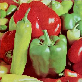
Algorithm 1: Coarse-to-fine stochastic ascent method for sampling from the implicit prior of a
denoiser, using denoiser residual f (y) = x̂(y) − y.
parameters: σ0 , σL , h0 , β
initialization: t = 1, draw y0 ∼ N (0.5, σ02 I)
while σt−1 ≤ σL do
     ht = 1+hh00(t−1)
                 t
                      ;
     dt = f (yt−1 );
               2
   σt2 = ||dNt || ;
   γt2 = (1 − βht )2 − (1 − ht )2 σt2 ;


   Draw zt ∼ N (0, I);
   yt ← yt−1 + ht dt + γt zt ;
   t←t+1
end

Figure 1: Sampling from the implicit prior embedded in BF-CNN trained on grayscale (two top rows)
and color (two buttom rows) Berkeley segmentation datasets. Each row shows a sequence of images,
yt , t = 1, 9, 17, 25, . . ., from the iterative sampling procedure, with different initializations, y0 , and
no added noise (β = 1).

Figure 1 illustrates the iterative generation of four images, starting from different random initializa-
tions, y0 , with no additional noise injected (i.e, β = 1), demonstrating the way that the algorithm
amplifies and "hallucinates" structure found in the initial (noise) images. Convergence is typically
achieved in less than 40 iterations with stochasticity disabled (β = 1). The left panel in Figure 2
shows samples drawn with different initializations, y0 , using a moderate level of injected noise
(β = 0.5). Images contain natural-looking features, with sharp contours, junctions, shading, and in
some cases, detailed texture regions. The right panel in Figure 2 shows a set of samples drawn with
more substantial injected noise (β = 0.1). The additional noise helps to avoid local maxima, and
arrives at images that are smoother and higher probability, but still containing sharp boundaries. As
expected, the additional noise also lengthens convergence time (see Figure 11). Figure 13 shows a set
of samples drawn from the implicit prior of a denoiser trained on the MNIST dataset of handwritten
digits.

                                                     5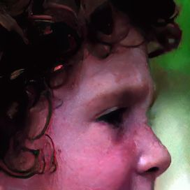
Figure 2: Samples arising from different inializations, y0 . Left: A moderate level of noise (β = 0.5)
is injected in each iteration. Right: A high level of injected noise (β = 0.1).

3         Solving linear inverse problems using the implicit prior

Many applications in signal processing can be expressed as linear inverse problems - deblurring, super-
resolution, estimating missing pixels (e.g., inpainting), and compressive sensing are all examples.
Given a set of linear measurements of an image, xc = M T x, where M is a low-rank measurement
matrix, one attempts to recover the original image. In Section 2, we developed a stochastic gradient-
ascent algorithm for obtaining a high-probability sample from p(x). Here, we modify this algorithm
to solve for a high-probability sample from the conditional density p(x|M T x = xc ).

3.1       Constrained sampling algorithm

Consider the distribution of a noisy image, y, conditioned on the linear measurements, xc = M T x,

                  p(y|xc ) = p(y c , y u |xc ) = p(y u |y c , xc )p(y c |xc ) = p(y u |xc )p(y c |xc )

where y c = M T y, and y u = M̄ T y (the projection of y onto the orthogonal complement of M ).
Without loss of generality, we assume the measurement matrix has singular values that are equal to
one (i.e., columns of M are orthogonal unit vectors, and thus M T M = I)2 . It follows that M is the
pseudo-inverse of M T , and that matrix M M T can be used to project an image onto the measurement
subspace. As with the algorithm of Section 2, we wish to obtain a local maximum of this function
using stochastic coarse-to-fine gradient ascent. Applying the operator σ 2 ∇ log yields

                      σ 2 ∇y log p(y|xc ) = σ 2 ∇y log p(y u |xc ) + σ 2 ∇y log p(y c |xc ).

The second term is the gradient of the observation noise distribution, projected into the measurement
space. If this is Gaussian with variance σ 2 , it reduces to M (y c − xc ). The first term is the gradient
of a function defined only within the subspace orthogonal to the measurements, and thus can be
computed by projecting the measurement subspace out of the full gradient. Combining these gives:

                       σ 2 ∇y log p(y) = (I − M M T )σ 2 ∇y log p(y) + M (xc − y c )
                                         = (I − M M T )f (y) + M (xc − M T y).                           (9)

Thus, we see that the gradient of the conditional density is partitioned into two orthogonal components,
capturing the gradient of the (log) noisy density, and the deviation from the constraints, respectively.
To draw a high-probability sample from p(x|xc ), we use the same algorithm described in Section 2,
substituting Eq. (9) for the deterministic update vector, f (y) (see Algorithm 2, and Figure 9).

      2
    The assumption that M has orthogonal columns does not restrict our solution. Assume an arbitrary linear
constraint, W T x = xw , and the singular value decomposition W = U SV T . Setting M = U , the constraint
holds if and only if M T x = xc , where xc = S # V T xw . The columns of M are orthogonal unit vectors,
M T M = I, and M M T is a projection matrix.

                                                           6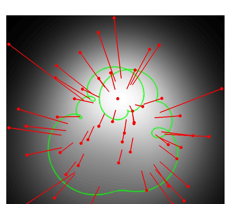
Algorithm 2: Coarse-to-fine stochastic ascent method for sampling from p(x|M T x = xc ), based
on the residual of a denoiser, f (y) = x̂(y) − y. Note: e is an image of ones.
parameters: σ0 , σL , h0 , β, M , xc
initialization: t=1; draw y0 ∼ N (0.5(I − M M T )e + M xc , σ02 I)
while σt−1 ≤ σL do
     ht = 1+hh00(t−1)
                 t
                      ;
     dt = (I − M M T )f (yt−1 ) + M (xc − M T yt−1 );
               2
   σt2 = ||dNt || ;
   γt2 = (1 − βht )2 − (1 − ht )2 σt2 ;


   Draw zt ∼ N (0, I);
   yt ← yt−1 + ht dt + γt zt ;
   t←t+1
end

Figure 3: Inpainting examples generated using three BF-CNN denoisers trained on (1) MNIST, (2)
Berkeley grayscale segmentation dataset (3) Berkeley color segmentation dataset. Left: original
images. Next: partially measured images. Right three columns: Restored examples, with different
random initializations, y0 . Each initialization results in a different restored image, corresponding to a
different point on the intersection of the manifold and the constraint hyper plane.

3.2   Linear inverse examples

We demonstrate the results of applying our method to several linear inverse problems. The same
algorithm and parameters are used on all problems - only the measurement matrix M and measured
values M T x are altered. In particular, as in section 2.1, we used BF-CNN [31], and chose parameters
σ0 = 1, σL = 0.01, h0 = 0.01, β = 0.01. For each example, we show a row of original images (x),
a row of direct least-squares reconstructions (M M T x), and a row of restored images generated by
our algorithm. For these applications, comparisons to ground truth are not particularly meaningful, at
least when the measurement matrix is of very low rank. In these cases, the algorithm relies heavily
on the prior to "hallucinate" the missing information, and the goal is not so much to reproduce the
original image, but to create an image that looks natural while being consistent with the measurements.
Thus, the best measure of performance is a judgement of perceptual quality by a human observer.
Inpainting. A simple example of a linear inverse problem involves restoring a block of missing
pixels, conditioned on the surrounding content. Here, the columns of the measurement matrix M are
a subset of the identity matrix, corresponding to the measured (outer) pixel locations. We choose a
missing block of size 30 × 30 pixels, which is less than the size of the receptive field of the BF-CNN
network (40 × 40), the largest extent over which this denoiser can be expected to directly capture
joint statistical relationships. There is no single correct solution for this problem: Figure 3 shows

                                                    7
Figure 4: Inpainting examples. Top row: original images (x). Middle: Images corrupted with blanked
region (M M T x). Bottom: Images restored using our algorithm.

      Figure 5: Recovery of randomly selected missing pixels. 10% of dimensions retained.

multiple samples, resulting from different initalizations. Each appears plausible and consistent with
the surrounding content. Figure 4 shows additional examples.
Random missing pixels. Consider a measurement process that discards a random subset of pixels.
M is a low rank matrix whose columns consist of a subset of the identity matrix corresponding to
the randomly chosen set of preserved pixels. Figure 5 shows examples with 10% of pixels retained.
Despite the significant number of missing pixels, the recovered images are remarkably similar to the
originals.

  Table 1: Spatial super-resolution results, averaged over images in Set5 (YCbCr-PSNR, SSIM)
                                              Algorithm
       Factor    MMT x           DIP            DeepRED         Ours            Ours - avg
       4:1       26.35, 0.826    30.04, 0.902   30.22, 0.904    29.47, 0.894    31.20, 0.913
       8:1       23.02, 0.673    24.98, 0.760   24.95, 0.760    25.07, 0.767    25.64, 0.792

                                                 8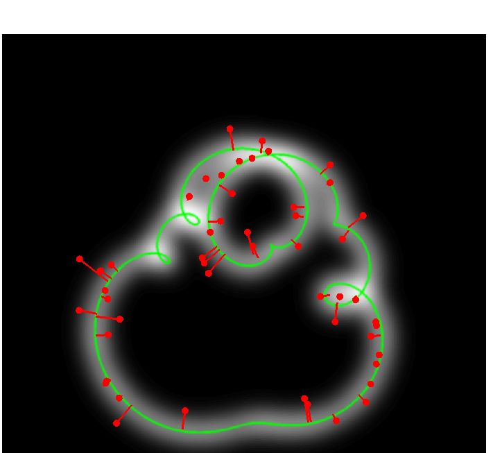
original      cropped        low res           DIP       DeepRED         Ours          Ours - avg
Figure 6: Spatial super-resolution. First and second column show three original images (full, and
cropped portion). Third column shows cropped portion with resolution reduced by averaging over
4x4 blocks (dimensionality reduction to 6.25%). Next three columns show reconstruction results
obtained using DIP [8], DeepRED [42], and our method. Last column shows an average over 10
samples from our method, which is blurrier but with better PSNR (see Tables 1 and 2).

 Table 2: Spatial super-resolution results, averaged over images in Set14 (YCbCr-PSNR, SSIM).
                                              Algorithm
        Factor   MMT x           DIP              DeepRED        Ours              Ours - avg
        4:1      24.65,0.765     26.88, 0.815     27.01, 0.817   26.56, 0.808      27.14, 0.826
        8:1      22.06, 0.628    23.33, 0.685     23.34, 0.685   23.32, 0.681      23.78, 0.703

Spatial super-resolution. In this problem, the goal is to construct a high resolution image from
a low resolution (i.e. downsampled) image. Downsampling is typically performed after lowpass
filtering, which determines the measurement model, M . Here, we use a 4 × 4 block-averaging
filter. For comparison, we also reconstructed high resolution images using Deep image Prior (DIP)
[8] and DeepRED [42]. DIP chooses a random input vector, and adjusts the weights of a CNN to
minimize the mean square error between the output and the corrupted image. The authors interpret
the denoising capability of this algorithm as arising from inductive biases imposed by the CNN
architecture that favor clean natural images over those corrupted by artifacts or noise. By stopping
the optimization early, the authors obtain surprisingly good solutions to the linear inverse problem.
Regularization by denoising (RED) develops a MAP solution, by using a least squares denoiser
as a regularizer [19]. DeepRED [42] combines DIP and RED, obtaining better performance than
either method alone. Results for three example images are shown in Figure 6. In all three cases,
our method produces an image that is sharper with less noticeable artifacts than the others. Despite
this, the PSNR and SSIM values are slightly worse (see Tables 1 and 2). These can be improved by
averaging over realizations (i.e., running the algorithm with different random initializations), at the
expense of some blurring (see last column of Figure 6). We can interpret this in the context of the
prior embedded in our denoiser: if each super-resolution reconstruction corresponds to a point on the
(curved) manifold of natural images, then the average (a convex combination of those points) will lie

Table 3: Run time (in seconds) for super-resolution algorithm, averaged over images in Set14, on an
NVIDIA DGX GPU.
                                             Algorithm
                                Factor    DIP       DeepRED      Ours
                                4:1       1,190     1,584        9

                                                   9
Figure 7: Deblurring (spectral super-resolution). Images blurred by retaining only 10% of low
frequencies.

off the manifold. This illustrates the point made earlier that comparison to ground truth (e.g. PSNR,
SSIM) is not particularly meaningful when the measurement matrix is very low-rank. Finally, our
method is more than two orders of magnitude faster than either DIP or DeepRED, as can be seen
from average execution times provided in Table 3.
Deblurring (spectral super-resolution). The applications described above are based on partial
measurements in the pixel domain. Here, we consider a blurring operator that operates by retaining a
set of low-frequency coefficient in the Fourier domain, discarding the rest. In this case, M consists
of the preserved low-frequency columns of the discrete Fourier transform, and M M T x is a blurred
version of x. Examples are shown in Figure 7.
Compressive sensing. Compressive sensing [44, 45] provides a set of theoretical results regarding
recovery of sparse signals from a small number of linear measurements. Specifically, if one assumes
that signals can be represented with at most k
31.1, 0.96       34.6, 0.99       36.7, 0.98        22.8, 0.78        25.2, 0.83       24.6, 0.77

    22.7, 0.73       24.7, 0.71       27.4, 0.79         17.1, 0.41       19.9, 0.47       19.8, 0.49

    23.4, 0.76       27.6, 0.86       30.4, 0.90         16.2, 0.40       19.5, 0.51       17.5, 0.43
Figure 8: Compressive sensing. Measurement matrix M contains random, orthogonal unit vectors,
with dimensionality reduced to 30% for the first three columns, and 10% for last three columns. As
in previous figures, top row shows original images (x), and second row is linear (pseudo-inverse)
reconstruction (M M T x). Third row: images recovered using our method. Fourth row: standard
compressive sensing solutions, assuming a sparse DCT signal model. Last row: standard compressive
sensing solutions, assuming a sparse wavelet (db3) signal model. Numbers indicate performance, in
terms of PSNR (dB), and SSIM [43].

to draw high-probability samples from its implicit prior, and a constrained variant that can be used to
solve any linear inverse problem. The derivation relies on the denoiser being optimized for mean
squared error in removing additive Gaussian noise of unspecified amplitude. Denoisers can be trained
using discriminative learning (nonlinear regression) on virtually unlimited amounts of unlabeled data,
and thus, our method extends the power of supervised learning to a much broader set of problems,
without further training.
Our method is similar to recent work that uses Score Matching to draw samples from an implicit
prior [14–18], but differs in several important ways: (1) Our derivation is direct and significantly
simpler, exploiting a little-known result from the classical statistical literature on Empirical Bayes
estimation [20]; (2) our method assumes a single (universal) blind denoiser, rather than a family of
denoisers trained for different noise levels; (3) our algorithm is efficient - we use stochastic gradient
ascent to maximize probability, rather than MCMC methods (such as Langevin dynamics) to draw
proper samples from each of a discrete sequence of densities; (4) convergence is fast, reliable and
robust, since step sizes are automatically adapted by the denoiser to be proportional to the distance to
the manifold. We’ve demonstrate the generality of our algorithm by applying it to five different linear
inverse problems.

                                                   11
Another related line of research uses a denoiser to regularize an objective function for solving
linear inverse problems [19, 42]. Our method differs in that (1) the term arising from our denoiser
represents the exact gradient of the (noisy) prior (it is not derived as an approximation); (2) our
method requires only that the denoiser be trained on Gaussian-noise contaminated images to minimize
squared error and must operate "blind" (without knowledge of noise level), whereas RED relies on a
set of three additional assumed properties; (3) RED has been used to solve MAP estimation problems,
whereas we have only applied our method to deterministic linear inverse problems (although we
believe it can be generalized to MAP); and (4) our algorithm has two primary hyper-parameters
(h0 and β) to control step sizes, and is robust to choices of these (see Appendix), whereas RED
includes multiple hyper-parameters, including the gradient step size whose adjustment is important
for achieving convergence (the issue is resolved through use of an ADMM method). Finally, we note
that DeepRED is derived to minimize MSE, and achieves better PSNR levels than our method, at the
expense of more blurring (see Fig. 6).
As mentioned previously, the performance of our method is not well-captured by comparisons to the
original image (using, for example, PSNR or SSIM). Performance should ultimately be quantified
using experiments with human observers, but might also be quantified using a no-reference perceptual
quality metric (e.g., [47]). Handling of nonlinear inverse problems with convex measurements (e.g.
recovery from quantized representation, such as JPEG) is a natural extension of the method, in which
the algorithm must be modified to incorporate projection onto convex sets. Finally, our method for
image generation offers a means of visualizing and interpreting implicit prior of a denoiser, which
arises from the combination of architecture, optimization, regularization, and training set. As such, it
offers a means of experimentally isolating and elucidating the effects of these components.
References
[1] D Donoho. Denoising by soft-thresholding. IEEE Trans Info Theory, 43:613–627, 1995.
[2] E P Simoncelli and E H Adelson. Noise removal via Bayesian wavelet coring. In Proc 3rd
IEEE Int’l. Conf. on Image Processing (ICIP), pages 379–382, 1996.
[3] P Moulin and J Liu. Analysis of multiresolution image denoising schemes using a generalized
Gaussian and complexity priors. IEEE Trans Info Theory, 45:909–919, 1999.
[4] Hyvärinen. Sparse code shrinkage: Denoising of nonGaussian data by maximum likelihood
estimation. Neural Computation, 11(7):1739–1768, 1999.
[5] J. Romberg, H. Choi, and R. Baraniuk. Bayesian tree-structured image modeling using wavelet-
domain hidden Markov models. IEEE Trans Image Proc, 10(7), July 2001.
[6] L Şendur and I W Selesnick. Bivariate shrinkage functions for wavelet-based denoising
exploiting interscale dependency. IEEE Trans Signal Proc, 50(11):2744–2756, November 2002.
[7] J Portilla, V Strela, M J Wainwright, and E P Simoncelli. Image denoising using scale mixtures
of Gaussians in the wavelet domain. IEEE Trans Image Proc, 12(11):1338–1351, Nov 2003.
Recipient, IEEE Signal Processing Society Best Paper Award, 2008.
[8] D Ulyanov, A Vedaldi, and V Lempitsky. Deep image prior. Proc Int’l J Computer Vision,
pages 1867–1888, April 2020.
[9] Ian Goodfellow, Jean Pouget-Abadie, Mehdi Mirza, Bing Xu, David Warde-Farley, Sherjil
Ozair, Aaron Courville, and Yoshua Bengio. Generative adversarial nets. In Advances in neural
information processing systems, pages 2672–2680, 2014.
[10] Viraj Shah and Chinmay Hegde. Solving linear inverse problems using GAN priors: An
algorithm with provable guarantees. 2018 IEEE Int’l. Conf. on Acoustics, Speech and Signal
Processing (ICASSP), Apr 2018.
[11] Ashish Bora, Ajil Jalal, Eric Price, and Alexandros G. Dimakis. Compressed sensing using
generative models, 2017.
[12] Eitan Richardson and Yair Weiss. On GANs and GMMs. In Advances in Neural Information
Processing Systems, pages 5847–5858, 2018.
12[13] Diederik P Kingma and Max Welling. Auto-encoding variational Bayes. In Second Int’l. Conf.
on Learning Representations (ICLR), volume 19, 2014.
[14] Y Bengio, L Yao, G Alain, and P Vincent. Generalized denoising auto-encoders as generative
models. In Adv. Neural Information Processing Systems (NIPS*13), pages 899–907. MIT Press,
2013.
[15] Saeed Saremi, Bernhard Schölkopf, Arash Mehrjou, and Aapo Hyvärinen. Deep energy
estimator networks. ArXiv e-prints (arXiv.org), 1805.08306, May 2018.
[16] Zengyi Li, Yubei Chen, and Friedrich T. Sommer. Learning energy-based models in high-
dimensional spaces with multi-scale denoising score matching, 2019.
[17] Yang Song and Stefano Ermon. Generative modeling by estimating gradients of the data
distribution. In Advances in Neural Information Processing Systems 32, pages 11918–11930.
Curran Associates, Inc., 2019.
[18] Siavash A Bigdeli, Geng Lin, Tiziano Portenier, L Andrea Dunbar, and Matthias Zwicker. Learn-
ing generative models using denoising density estimators. arXiv preprint arXiv:2001.02728,
2020.
[19] Yaniv Romano, Michael Elad, and Peyman Milanfar. The little engine that could: Regularization
by denoising (RED). CoRR, abs/1611.02862, 2017.
[20] K Miyasawa. An empirical Bayes estimator of the mean of a normal population. Bull. Inst.
Internat. Statist., 38:181–188, 1961.
[21] J J Koenderink. The structure of images. Biological Cybernetics, 50:363–370, 1984.
[22] T Lindeberg. Scale-space theory: A basic tool for analysing structures at different scales.
Journal of Applied Statistics, 21(2):224–270, 1994.
[23] Norbert Wiener. Extrapolation, interpolation, and smoothing of stationary time series: with
engineering applications. Technology Press, 1950.
[24] Y. Hel-Or and D. Shaked. A discriminative approach for wavelet shrinkage denoising. IEEE
Trans. Image Processing, 17(4), April 2008.
[25] Michael Elad and Michal Aharon. Image denoising via sparse and redundant representations
over learned dictionaries. IEEE Trans. on Image processing, 15(12):3736–3745, 2006.
[26] Viren Jain and Sebastian Seung. Natural image denoising with convolutional networks. In
Advances in neural information processing systems, pages 769–776, 2009.
[27] Harold C Burger, Christian J Schuler, and Stefan Harmeling. Image denoising: Can plain neural
networks compete with BM3D? In Proc. IEEE Conf. Computer Vision and Pattern Recognition
(CVPR), pages 2392–2399. IEEE, 2012.
[28] Kai Zhang, Wangmeng Zuo, Yunjin Chen, Deyu Meng, and Lei Zhang. Beyond a Gaussian
denoiser: Residual learning of deep CNN for image denoising. IEEE Trans. Image Processing,
26(7):3142–3155, 2017.
[29] Gao Huang, Zhuang Liu, Laurens Van Der Maaten, and Kilian Q Weinberger. Densely connected
convolutional networks. In Proc. IEEE Conf. Computer Vision and Pattern Recognition (CVPR),
pages 4700–4708, 2017.
[30] Yunjin Chen and Thomas Pock. Trainable nonlinear reaction diffusion: A flexible framework
for fast and effective image restoration. IEEE Trans. Patt. Analysis and Machine Intelligence,
39(6):1256–1272, 2017.
[31] S Mohan*, Z Kadkhodaie*, E P Simoncelli, and C Fernandez-Granda. Robust and interpretable
blind image denoising via bias-free convolutional neural networks. In Int’l. Conf. on Learning
Representations (ICLR), Addis Ababa, Ethiopia, April 2020.
13[32] Saeed Saremi and Aapo Hyvarinen. Neural empirical Bayes. Journal of Machine Learning
Research, 20:1–23, 2019.
[33] Zengyi Li, Yubei Chen, and Friedrich T Sommer. Annealed denoising score matching: Learning
energy-based models in high-dimensional spaces. arXiv preprint arXiv:1910.07762, 2019.
[34] H Robbins. An empirical Bayes approach to statistics. Proc. Third Berkley Symposium on
Mathematcal Statistics, 1:157–163, 1956.
[35] M Raphan and E P Simoncelli. Least squares estimation without priors or supervision. Neural
Computation, 23(2):374–420, Feb 2011.
[36] B D Lucas and T Kanade. An iterative image registration technique with an application to stereo
vision. In Proc. 7th Int’l Joint Conf. on Artificial Intelligence, pages 674–679, Vancouver, 1981.
[37] S. Kirkpatrick, C. D. Gelatt, and M. P. Vecchi. Optimization by simulated annealing. Science,
220(4598):671–680, 1983.
[38] S. Geman and D. Geman. Stochastic relaxation, Gibbs distributions, and the Bayesian restoration
of images. IEEE Trans Pattern Analysis and Machine Intelligence, 6(6):721–741, 1984.
[39] A. Blake and A. Zisserman. Visual Reconstruction. MIT Press, 1987.
[40] D. Martin, C. Fowlkes, D. Tal, and J. Malik. A database of human segmented natural images
and its application to evaluating segmentation algorithms and measuring ecological statistics.
In Proc. 8th Int’l Conf. Computer Vision, volume 2, pages 416–423, July 2001.
[41] Yann LeCun and Corinna Cortes. MNIST handwritten digit database.
http://yann.lecun.com/exdb/mnist/, 2010.
[42] Gary Mataev, Peyman Milanfar, and Michael Elad. Deepred: Deep image prior powered by red.
In Proceedings of the IEEE International Conference on Computer Vision Workshops, pages
0–0, 2019.
[43] Z Wang, A C Bovik, H R Sheikh, and E P Simoncelli. Perceptual image quality assessment:
From error visibility to structural similarity. IEEE Trans Image Processing, 13(4):600–612, Apr
2004.
[44] Emmanuel J Candès, Justin K Romberg, and Terence Tao. Stable signal recovery from in-
complete and inaccurate measurements. Communications on Pure and Applied Mathematics,
59(8):1207–1223, 2006.
[45] D. L. Donoho. Compressed sensing. IEEE Trans Info Theory, 52(4):1289–1306, 2006.
[46] T. Blumensath and M. E. Davies. Sampling theorems for signals from the union of finite-
dimensional linear subspaces. IEEE Transactions on Information Theory, 55(4):1872–1882,
2009.
[47] K. Ma, W. Liu, K. Zhang, Z. Duanmu, Z. Wang, and W. Zuo. End-to-end blind image quality
assessment using deep neural networks. IEEE Transactions on Image Processing, 27(3):1202–
1213, 2018.
[48] Yann LeCun, Corinna Cortes, and CJ Burges. Mnist handwritten digit database. ATT Labs
[Online]. Available: http://yann.lecun.com/exdb/mnist, 2, 2010.
14A Description of BF-CNN denoiser
Architecture. Throughout the paper, we use BF-CNN, described in [31], constructed from 20
bias-free convolutional layers, each consisting of 3 × 3 filters and 64 channels, batch normalization,
and a ReLU nonlinearity. Note that to construct a bias-free network, we remove all sources of additive
bias, including the mean parameter of the batch-normalization in every layer.
Training Scheme. We follow the training procedure described in [31]. The network is trained to
denoise images corrupted by i.i.d. Gaussian noise with standard deviations drawn from the range
[0, 0.4] (relative to image intensity range [0, 1]). The training set consists of overlapping patches of
size 40 × 40 cropped from the Berkeley Segmentation Dataset [40]. Each original natural image is of
size 180 × 180. Training is carried out on batches of size 128, for 70 epochs.
B Block diagram of Universal Inverse Sampler
✓0
MSE r✓ + +
+
training
distribution z
D✓ (·)
x MT xc ✓ˆ
M + T
D✓ (·)
- M
x̂ ⇠ p(x|xc )
+ +
- y0
dt
+ y
+
t
|| · ||
p h(·) (·)
+
N
t
h0 z
Figure 9: Block diagrams for denoiser training, and Universal Inverse Sampler. Top: A parametric
blind denoiser, Dθ (·), is trained to minimize mean squared error when removing additive Gaussian
white noise (z) of varying amplitude (σ) from images drawn from a training distribution. The
trained denoiser parameters, θ̂, constitute an implicit model of this distribution. Bottom: The trained
denoiser is embedded within an iterative computation to draw samples from this distribution, starting
from initial image y0 , and conditioned on a low-dimensional linear measurement of a test image:
x̂ ∼ p(x|xc ), where xc = M T x. If measurement matrix M is empty, the algorithm draws a sample
from the unconstrained distribution. Parameter h0 ∈ [0, 1] controls the step size, and β ∈ [0, 1]
controls the stochasticity (or lack thereof) of the process.
15C Visualization of Universal Inverse Sampler on a 2D manifold prior
Figure 10: Two-dimensional simulation/visualization of the Universal Inverse Sampler. Fifty example
signals x are sampled from a uniform prior on a manifold (green curve). First three panels show,
for three different levels of noise, the noise-corrupted measurements of the signals (red points), the
associated noisy signal distribution p(y) (indicated with underlying grayscale intensities), and the
least-squares optimal denoising solution x̂(y) for each (end of red line segments), as defined by
Eq. (2), or equivalently, Eq. (3). Right panel shows trajectory of our iterative coarse-to-fine inverse
algorithm (Algorithm 2, depicted in Figure 9), starting from the same initial values y (red points) of
the first panel. Algorithm parameters were h0 = 0.05 and β = 1 (i.e., no injected noise). Note that,
unlike the least-squares solutions, the iterative trajectories are curved, and always arrive at solutions
on the signal manifold.
D Convergence
Figure 11 illustrates the convergence of our iterative sampling algorithm, expressed in terms of
the effective noise standard deviation σ = ||d ||
√ t averaged over synthesis of three images, for three
N
different levels of the stochasticity parameter β. Convergence is well-behaved and efficient in all
cases. As expected, with smaller β (larger amounts of injected noise), effective standard deviation
falls more slowly, and convergence takes longer. For β = 1 (no injected noise), the convergence is
approximately what is expected from the formulation of the alorithm (Eq. 7). For larger amounts
of injected noise, the algorithm converges faster than expected, we believe because a portion of the
additive noise is parallel to the manifold, so does not contribute to calculated variance.
=1 = 0.1 = 0.01
1.0 empirical empirical empirical
expected expected expected
0.8
0.6
0.4
0.2
0.0
0 5 10 15 20 25 30 0 20 40 60 80 100 120 0 100 200 300 400 500 600
t t t
Figure 11: Comparison of the computed effective noise, σt = ||d ||
√ t , and the noise expected from the
N
schedule σt = (1 − βht )σt−1 , where ht = h0 1+h0t(t−1) . When β = 1, the effective noise estimated
by the denoiser falls at approximately the rate expected by the schedule. As β decreases (i.e. for
non-zero injected noise), convergence is slower, but faster than the expected rate.
In addition to the total effective noise, we can compare the evolution of the removed noise versus
injected noise. Figure 12 shows the reduction in effective standard deviation, ht σt = ht ||d ||
√ t in each
N
iteration, along with the standard deviation of the added noise, γt . The amount of noise added relative
to the amount removed is such that effective noise drops as σt = (1 − βht )σt−1 . When β = 1, the
addedtive noise is zero, γt = 0, and the convergence of σt is the fastest. When β = 0.01, a lot of
noise is added in each iteration, and the convergence is the slowest.
16=1 = 0.1 = 0.01
1.0 1.0 1.0
ht||dNt||
0.8 0.8 0.8
||zt||
t N
0.6 0.6 0.6
0.4 0.4 0.4
0.2 0.2 0.2
0.0 0.0 0.0
0 50 100 150 200 250 0 50 100 150 200 250 0 50 100 150 200 250
t t t
Figure 12: Temporal evolution of the amplitude of removed (solid) and injected (dashed) noise for
the same patches as in Figure 11. β = 1 corresponds to zero added noise (γt = 0), hence the fastest
convergence, while β = 0.01 corresponds to a high level of added noise, hence slower convergence.
E Sampling from the implicit prior of a denoiser trained on MNIST
Figure 13: Training BF-CNN on the MNIST dataset of handwritten digits [48] results in a different
implicit prior (compare to Figure 2). Each panel shows 16 samples drawn from the implicit prior,
with different levels of injected noise (increasing from left to right, β ∈ {1.0, 0.3, 0.01}).
17You can also read