Real-time Simultaneous Pose and Shape Estimation for Articulated Objects Using a Single Depth Camera
←
→
Page content transcription
If your browser does not render page correctly, please read the page content below
Real-time Simultaneous Pose and Shape Estimation
for Articulated Objects Using a Single Depth Camera
Mao Ye Ruigang Yang
mao.ye@uky.edu ryang@cs.uky.edu
University of Kentucky
Lexington, Kentucky, USA, 40506
Abstract
In this paper we present a novel real-time algorithm
for simultaneous pose and shape estimation for articu-
lated objects, such as human beings and animals. The
key of our pose estimation component is to embed the ar-
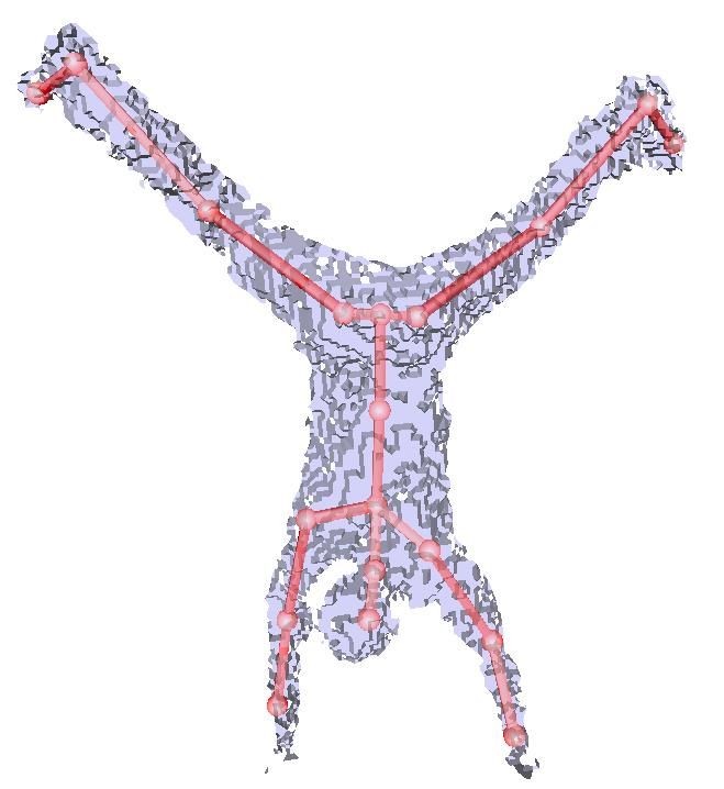
Figure 1. Our novel algorithm effectively estimates the pose of
ticulated deformation model with exponential-maps-based
articulated objects using one single depth camera, such as human
parametrization into a Gaussian Mixture Model. Benefiting
and dogs, even with challenging cases.
from the probabilistic measurement model, our algorithm
requires no explicit point correspondences as opposed to mum, especially in the case of fast and complex motions.
most existing methods. Consequently, our approach is less When a template model is used, as in generative or hybrid
sensitive to local minimum and well handles fast and com- approaches, the consistency of body shape (limb lengths
plex motions. Extensive evaluations on publicly available and girths) between the model and the subject is critical
datasets demonstrate that our method outperforms most for accurate pose estimation. Most existing approaches ei-
state-of-art pose estimation algorithms with large margin, ther require given shapes [11, 29], small variations from the
especially in the case of challenging motions. Moreover, template [12], or specific initialization [27, 13]. Apparently,
our novel shape adaptation algorithm based on the same these requirements limit the applicability of these methods
probabilistic model automatically captures the shape of the in home environments.
subjects during the dynamic pose estimation process. Ex- To overcome the limitations mentioned above, we pro-
periments show that our shape estimation method achieves pose a novel (generative) articulated pose estimation al-
comparable accuracy with state of the arts, yet requires nei- gorithm that does not require explicit point correspon-
ther parametric model nor extra calibration procedure. dences and captures the subject’s shape automatically
during the pose estimation process. Our algorithm relates
1. Introduction the observed data with our template using Gaussian Mix-
The topic of pose estimation for articulated objects, in ture Model (GMM), without explicitly building point corre-
particular human pose estimation [17, 22], has been actively spondences. The pose is then estimated through probability
studied by the computer vision community for decades. In density estimation under articulated deformation model pa-
recent years, due to the increasing popularity of depth sen- rameterized with exponential maps [2]. Consequently, the
sors, studies have been conducted to capture the pose of algorithm is less sensitive to local minimum and well ac-
articulated objects using one or more such depth sensors commodates fast and complex motions. In addition, we
(detailed in Sec. 2). Despite of the substantial progress that develop a novel shape estimation algorithm within the same
have been achieved, there are still various limitations. probabilistic framework that is seamlessly combined with
Discriminative approaches [23, 25, 21] in general are ca- our pose estimation component. Last but not the least, our
pable of handling large body shape variations. Yet it has pipeline is implemented on GPU with CUDA, and achieves
been shown that most existing discriminative and hybrid ap- real-time performance (> 30 frames per second).
proaches cannot achieve high accuracy with complex mo- We conduct extensive evaluations on publicly available
tions [13]. The majority of generative approaches require datasets. The experiments show that our algorithm outper-
building point correspondences, mostly with variants of ICP forms most existing methods [11, 23, 30, 1, 12, 13] with
methods. Thus they are prone to be trapped in local mini- large margin, especially in the case of complex motions.
1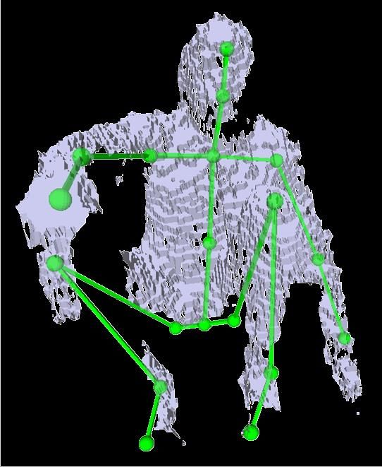
Our method is flexible enough to handle animals as well, as        accurately merged to obtain a complete shape [4]. How-
shown in Figure 1 and Figure 8.                                    ever, the noise from current depth sensors could downgrade
                                                                   the method’s accuracy by a large degree [5]. With a sin-
2. Related Work                                                    gle depth sensor, usually only the overall shapes are recov-
                                                                   ered [28, 13]. Compared to these methods, our approach
Pose Estimation from Depth Sensors The approaches                  does not require parametric models. Besides, our algorithm
for depth-based pose estimation can be classified into dis-        adapts the template shape to the subject’s automatically dur-
criminative, generative and hybrid approaches. Existing            ing the pose estimation process, without requiring the sub-
discriminative approaches either performed body part de-           ject to perform extra specific motions. Experiments show
tection by identifying salient points of the human body [20],      that our algorithm can deal with large shape variations.
or relied on classifiers or regression machines trained of-
fline to infer the joint locations [23, 25]. Shotton et al. [23]   3. GMM-based Pose and Shape Estimation
trained a Random Forest classifier for body part segmenta-
tion from a single depth image, and then estimated joint lo-          Our pose tracker uses a skinning mesh model as tem-
cations using mean shift algorithm. Also based on Random           plate. Specifically, the template consists of four compo-
Forest, Taylor et al. [25] directly inferred mode-to-depth         nents, the surface vertices V = {v 0m |m = 1, · · · , M },
correspondences for off-line pose optimization. As will be         the surface mesh connectivity F, the skeleton J and the
shown in Sec. 4, our algorithm achieves significantly higher       skinning weights A. In general, the hierarchy of the joints
accuracy in the case of complex motions compared to [23]           in the skeleton J forms a tree structure (kinematic tree).
and the KinectSDK [16].                                            The goal of pose estimation is to identify the pose Θ, under
    The generative approaches fit a template, either para-         which the deformed surface vertices, denoted as V(Θ) =
metric or non-parametric, to the observed data, mostly             {v Θ
                                                                      m |m = 0, · · · , M }, best explain the observed point
with variants of ICP. Ganapathi et al. [12] used Dynamic           cloud X = {xn |n = 1, · · · , N }.
Bayesian Network (DBN) to model the motion states and              3.1. The General Probabilistic Model
demonstrated good performance with an extend ICP mea-
surement model and free space constraint. Yet their over-              Our algorithm assumes that the observed point cloud X
simplified cylindrical template cannot capture the subject’s       follows a Gaussian Mixture Model (GMM) whose centroids
shape. The work by Gall et al. [9], built upon [10], used          are the deformed template vertices V(Θ). Similar to [19],
both depth and edge information to guide the tracker also          an extra uniform distribution is included to account for out-
within the ICP framework. Compared to this line of works,          liers. Therefore, the probability of each observed point
our method does not require explicit point correspondences         xn ∈ X can be expressed as
and is more robust in dealing with fast complex motions.                                     M
                                                                                             X                              1
    The complementary characteristics of these two groups                 p(xn ) = (1 − u)         p(v Θ          Θ
                                                                                                       m )p(xn |v m ) + u       (1)
                                                                                                                            N
of approaches have been combined to achieve higher accu-                                     m=1
racy. Ye et al. [30] and Baak et al. [1] use database lookup to                         1            −kx − v Θ k2
                                                                                                         n     m
locate a similar pose, with PCA of normalized depth images           p(xn |v Θ
                                                                             m) =               exp                             (2)
                                                                                    (2πσ 2 )d/2           2σ 2
and salient point detection, respectively. Helten et al. [13]
extended [1] to obtain personalized tracker that can handle        where d is the dimensionality of the point set (d = 3 in our
larger body shape variations and achieves real-time perfor-        case) and u is the weight of the uniform distribution that
mance. Ganapathi et al. [11] use body part detector [20]           roughly represents the percentage of the outliers in X . Here
to guide their tracker within the DBN framework. This              a single variance parameter σ 2 is used for all Gaussians for
DBN model is combined with the Random Forest classi-               simplicity. Similar to [19, 6], we assume uniform distribu-
fier [23] by Wei et al. [27] to achieve high accuracy with         tion for the prior, that is p(v Θ
                                                                                                   m ) = 1/M .
real-time performance. The generative component of these              Under this probabilistic mode, pose estimation is cast as
approaches [13, 11, 27] are also ICP-based.                        a probability density estimation problem that minimizes the
                                                                   following negative log-likelihood:
Shape Estimation The topic of shape estimation has also
                                                                                 N        M
been extensively studied, however mainly for rigid bod-                         X       X   1−u              u
                                                                   E Θ, σ 2 = −                  p(xn |v Θ

                                                                                    log                  m) +    (3)
ies [3, 15]. Some methods can deal with small degree                                          M               N
                                                                                n=1      m=1
of motions for articulated objects [28, 5, 31]. Only a
few methods allow the subject to perform free movements.           which is normally solved iteratively using the Expectation-
Using multi-view setup, detailed geometry can be recov-            Maximization (EM) algorithm [8]. During the E-step, the
ered [7, 26, 14, 24]. High quality monocular scans of              posteriors pold (v Θ
                                                                                      m |xn ) are calculated using the parameters
strictly articulated objects under different poses can also be     estimated from the previous iteration based on Bayes rule: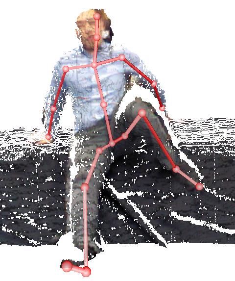
−kxn −v Θ 2
t
mk = I3 [v tm ]× ;
exp 2σ 2
where Im (11)
pmn ≡ pold (v Θ
m |xn ) = PM (4) XK
−kxn −v Θ δki αmi ; ξˆk0t = Tkt ξˆk (Tkt )−1
2
mk βmk = (12)
m=1 exp 2σ 2 + uc i=1
2 d/2 Here I3 is a 3 × 3 identity matrix, and the operator [·]×
where uc = (2πσ )
(1−u)N
uM
. During the M-step, the parame-
converts a vector to a skew-symmetric matrix. The weight
ters are updated via minimizing the following complete neg- βmk accumulates the corresponding skinning weights along
ative log-likelihood (upper bound of Eq. 3): all joints and represents the global influence of joint k over
1−u u
vertex v m . The term ξˆk0t is a coordinate transformed twist
X
Q Θ, σ 2 = − p(xn |v Θ
pmn log m ) + log
M N
n,m of ξˆk via the transformation of joint k, namely Tkt .
1 X d
∝ 2
pmn kxn − v Θ 2
m k + P log σ
2
(5) 3.3. The Tracking Algorithm
2σ n,m 2
X X XN XM The core of our tracking algorithm is the combination
where P = pmn ; ≡ (6) of the articulated deformation model in Sec. 3.2 with the
n=1 m=1
n,m n,m probabilistic framework in Sec. 3.1. Plugging Eq. 10 into
So far, the probabilistic model is independent of the form Eq. 5, we get the following objective function (superscript
of deformation model in V(Θ). Cui et al. [6] and Myro- ignored for notational simplicity):
nenko et al. [19] used this model for rigid and non-rigid 1 X
Q(∆Θ, σ 2 ) = pmn kxn − v m − Im ∆ξ g
point set registration. Different from their work, we derive 2σ 2 n,m
the pose estimation formulation under the articulated defor-
K d
mation model, which is more suitable for a large variety of X
− βmk ξˆk0 v m ∆θk k2 + P log σ 2
articulated-like objects (e.g., human and many animals). 2
k=1
3.2. Twist-based Articulated Deformation Model X pmn d
= kxn − v m − Am ∆Θk2 + P log σ 2 (13)
We use twist and exponential maps to represent the 3D
n,m
2σ 2 2
transformations of each joint in the skeleton, similar to [2,
where Am = Im βm1 ξˆ10 v m · · · βmK ξˆK 0
10, 13]. With this parametrization, the transformation of a vm (14)
joint in the kinematic tree can be represented as: T T
YK ∆Θ = ∆ξ g ∆θ1 · · · ∆θK (15)
Ti = eξ̂g eδki ξ̂k θk (7) 2
In order to solve for the parameters {∆Θ, σ }, the par-
k=1
tial derivatives of Q(∆Θ, σ 2 ) over the parameters are set
1 joint k is an ancestor of joint i
n
where δki = (8) to zero to obtain the following equations:
0 otherwise X pmn X pmn
ATm Am ∆Θ = ATm (xn − v m ) (16)
Here ξˆg and ξˆk θk represent the global transformation and n,m
σ 2
n,m
σ 2
local rotation of joint k respectively (see [18] for details). 1 X
Without loss of generality, we assume the index of a joint is σ2 = pmn kxn − v m k2 (17)
dP n,m
smaller than its children throughout this paper.
The skinning model deforms a vertex vm ∈ V with the These two equations comprise the core of our novel
weighted sum of the transformations of its controlling joints tracking algorithm. To better regularize the optimization,
as follows: K we add the following two terms to the objective function:
X
vΘ
m = αmk TiΘ v 0m (9) Er (∆Θ) = k∆Θk2 (18)
k=1 K t
X X 2
where {αmk ∈ A} are the skinning weights from our tem- Ep (∆Θ) = θkprev + ∆θτk − θkpred (19)
plate. Notice that throughout the texts, homogeneous and k=1 τ =1
inhomogeneous coordinates are used interchangeably with- The term Er ensures that the solution complies with
out explicit differentiation for notational simplicity. the small pose change assumption during linearization in
As shown in Section 3.1, the pose will be updated in Eq. 10. In Ep , {θkprev } are the joint angles from previous
an iterative fashion. At iteration t, with the assumption of frame, and {θkpred } are the predicted joints angles using lin-
small changes of both joints angles {∆θkt } and global trans- ear third order autoregression similar to [10]. The second
formation ∆ξ tg , the deformation model in Eq. 9 can be lin- term penalizes a solution’s large deviation from the pre-
earized (see supplemental materials for derivation): diction, assuming relatively continuous motions in tracking
XK scenario. This term is helpful in dealing with occlusions, in
v t+1
m ≈ v t
m + I t
m ∆ξ t
g + βmk ξˆk0t v tm ∆θkt (10) which case the joints corresponding to invisible parts can be
k=1 relatively well constrained.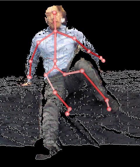
Initialize the template with previous pose                         begin Step One
   Sample a subset of points from each point set                          Exclude template points outside the camera view;
   while Pose not converged do                                            Perform Alg. 1;
        E-step: Compute posteriors via Eq. 4.                         end
        M-Step:                                                       begin Step Two
           • Minimize Eq. 20 for (∆Θ, σ 2 ).                              Perform visibility test and exclude invisible points
           • Update template vertices via Eq. 9.                          from the template;
   end                                                                    Perform Alg. 1;
                                                                      end
     Algorithm 1: The pose estimation procedure.
                                                                      Algorithm 2: Pose estimation for monocular data.
   Our complete objective function is the weighted sum of
                                                                    view limitation. By using only visible points in the second
these three terms:
                                                                    refining step, these two issues could be partially resolve, as
    E = Q(∆Θ, σ 2 ) + λr Er (∆Θ) + λp Ep (∆Θ)              (20)     the joint angles of the corresponding invisible parts will not
   The partial derivative of Er and Ep over ∆Θ are added            be updated. However, they might still be affected during the
to Eq. 16 and the entire linear system is solved at each it-        first step. Therefore, we limit our sampling candidates to the
eration for the pose update ∆Θ. Eq. 17 is solved for the            set of template vertices inside the camera view. Besides, we
Gaussian variance σ 2 . After each pose update, the sur-            rely on the autoregression prediction in Eq. 19 to constraint
face vertices are updated via the skinning deformation in           the occluded parts that are inside the camera view. With
Eq. 9. In the E-step, the posteriors are calculated according       these strategies, our algorithm can effectively and reliably
to Eq. 4. The procedure iterates until the maximum surface          estimate the pose using only one single depth camera. The
vertex movements is below a certain threshold (1mm in our           entire pose estimation procedure is summarized in Alg. 2.
experiments). Note that the small pose update is only en-           3.5. Template Shape Adaptation and Initialization
forced between two iterations, while large pose change
between two frames is allowed (see our video).                          The consistency of body shape (limb lengths and body
   Since the computational complexity is in the order of            part girths) between the template and the subject plays a
M N , we use only a subset from each point cloud during             critical role in pose estimation. In this section, we describe
the optimization. For the template mesh, random sampling            our novel algorithm for automatic body shape estimation,
strategy is used. The observed point set is uniformly sub-          followed by the initialization procedure of our tracker.
sampled based on the regular image grid. The pose estima-           3.5.1    Limb Lengths Estimation
tion process for each new frame is summarized in Alg. 1.
                                                                    In order to adjust the limb lengths of template to fit the sub-
3.4. Monocular Scenario                                             ject, existing methods either assume presence of a person-
    In monocular setup, the missing data introduces addi-           alized template model [10] or estimate the body size before
tional difficulties for the algorithm above. Specifically the       tracking [27, 13]. We follow the later strategy because ap-
algorithm attempts to use all given template vertices to fit        parently it is more general. However, our method requires
the observed data. However, since the template surface is           neither parametric model as in [13], nor body part detectors
complete while the observed surface is partial, the observed        as in [27]. Instead, we parameterize the template vertices on
partial surface will typically end up inside the complete           limb lengths and utilize the probabilistic model in Sec. 3.1
template surface (between frontal and back surfaces). An            to estimate the optimal body size.
intuitive strategy is to use only the visible part of the tem-          To achieve linear parametrization, we adopt the differen-
plate from previous frame, as being adopted by Helten et            tial bone coordinates introduced by Straka et al. [24], which
al. [13]. However, such strategy can not well handle rota-          is defined in a way similar to the Laplacian coordinates:
                                                                           K
tion of body parts, as the visible parts will change. Towards             X
this end, we propose a two-step coarse-to-fine strategy to         ηm =        αmk η mk ; η mk = v m −(g k −(1−γmk )dk ) (21)
                                                                            k=1
handle this situation. In the first step, the entire set of tem-
plate vertices are used for sampling, and the pose are up-          As explained in Fig. 2, the local geometric shape informa-
dated until convergence. In most cases, the body parts will         tion is encoded inside these coordinates.
be very close to their correct places. Then the visibility of          The adjustment of the limb lengths are achieved by in-
the template surface is determined and only the visible part        troducing a scale for each bone, denoted as S = {sk }. The
are used to refine the pose.                                        scaled bone vectors become {sk dk }, assuming unchanged
    Another type of missing data is the occlusion of an entire      pose. Consequently, the scaled joint positions can be com-
body segment, either due to self occlusion or camera field of       puted as: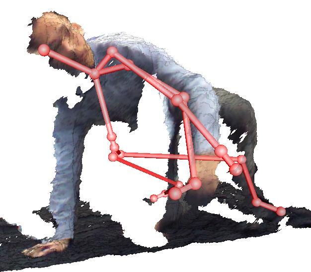
1                          while Scales not converged do
                                                                               Estimate pose Θ using Alg. 2;
                                                                               Calculate the joints {g k , g r } and {dk } from Θ;
                                                                               Compute {η m } according to Eq. 21;
Figure 2. The differential bone coordinates [24]. g k is the location          Estimate scales S via Eq. 26 and Eq. 27;
of joint k and dk is the vector from parent of joint k to itself. Each         Update the template with the scales S
vector η m,k encodes the relative position of the vertex v m with re-      end
spect to bone k. The differential bone coordinate defined in Eq. 21
                                                                           Algorithm 3: Limb lengths estimation procedure.
accumulates such relative positions along all controlling bones of
this vertex and encodes the information of surface geometry.
                                                                         summarized in Alg. 3. The effectiveness of our template
                                  XK
                g k (S) = g r +                δjk sj dj         (22)    limb length adaptation is illustrated in Fig. 9 and our sup-
                                         j=1                             plemental video.
where g r is the position of the root that only changes with
pose. Combining Eq. 22 and Eq. 21, we can reconstruct the                3.5.2   Geometric Shape Adaptation
vertex positions for the scaled template with the following
equation:                                                                Besides limb length adaptation, we further develop an auto-
                                   XK                                    matic method to capture the overall geometry of the subject
           v m (S) = η m + g r +           ρmk sk dk    (23)
                                               k=1                       directly inside the pose estimation process, which does not
     where     ρmk = βmk − αmk (1 − γmk )                        (24)    require the subject to perform any additional specific mo-
                                                                         tions as in [13]. The key insight is that upon convergence of
   The idea of our limb lengths adaptation is to estimate
                                                                         pose estimation, the maximum of posteriors p(v m |xn ) over
the scales, such that the vertices of the scaled template de-
                                                                         all {xn } naturally provide information about the point cor-
fined in Eq. 23 maximizes the objective function defined in
                                                                         respondences. Moreover, the corresponding posteriors can
Eq. 13. Therefore, plugging Eq. 23 into Eq. 13 and chang-
                                                                         serve as a measure of uncertainty. With a sequence of data,
ing the unknown from pose to the scales, we obtain the fol-
                                                                         we can treat each such correspondence as an observed sam-
lowing objective function for limb length scales estimation:
                      K                                                  ples of our target adapted surface vertex v̂ m . Consequently,
          X pmn  X
Q(S) =                   ρ    s  d  +  η   + g   − x     (25)            the weighted average over all the samples can be used to
                           mk  k  k      m     r     n
          nm
              2σ 2                                                       represent our adapted template:
                       k=1                                                                                    .X
                                                                                          X
Again, setting the partial derivatives of the above objective                      v̄ m =      ω(xf(m) )xf(m)         ω(xf(m) )   (28)
                                                                                              f                    f
function over the scales to zero yields:
    XK  1
                   T
                        X                       dTk                     where   xf(m)   is the correspondence identified via maximum
                 d k dj     p mn ρ mj ρmk   sj =     ·
       j=1 σ 2
                        n,m
                                                 σ2                      of posteriors at frame f . The weight ω(xf(m) ) is designed
    X                                                                    to take into account both the uncertainty based on the pos-
        pmn ρmk (xn − η m − g r ); k = 1, · · · , K (26)                 terior and the sensor noise based on depth, and is defined as
    n,m
                                                                         follows:
   In order to assure a reasonable overall shape of the scaled                         ω(xf(m) ) = p(v m |xf(m) ) [xf(m) ]2z

                                                                                                                                  (29)
template, we further enforce consistency of the estimated
scales for a set of joints pairs:                                        where the quantity [·]z denotes the z (depth) component.
                                                                            In order to ensure smoothness of final adapted surface
             λs ωi,j si = λs ωi,j sj ;     < i, j >∈ B           (27)
                                                                         and to further handle noises, we allow the movement of a
Here the global weight λs leverages the relative importance              surface vertex only along its original normal. Consequently,
of this regularization term with respect to the data term in             a displacement dm is estimated for each vertex v m , by op-
Eq. 26, and ωi,j represents the relative strength of the sim-            timizing the following objective function:
ilarity for the pair (si , sj ) among others. For human and                     XM
animals, we set ωi,j = 1 for symmetric parts (e.g left/right             Ed =             ωm kdm nm − (v̄ m − v 0m )k2 + λd kdm k2
                                                                                   m=1
arm) and 0.5 for connected bones. Combining Eq. 26 and
                                                                                     X
                                                                             + λe           kdm − dl k2                         (30)
Eq. 27, we can solve for the scales so that the template is                        ∈F
best fit to the observed points under our probabilistic model.
    Notice that the parametrization in Eq. 23 requires un-               where the weight ωm = 1 if the vertex has correspondence
changed pose. However, before the template is appropri-                  up to the current frame and 0 otherwise. The first term
ately scaled, the pose might not be well estimated. There-               moves the vertex to the projection of the weighted sum de-
fore, we iterate between pose estimation and scale estima-               fined in Eq. 28 on the normal nm . The second term penal-
tion until the estimated scales converge. The procedure is               izes large movements and the third one enforces smoothness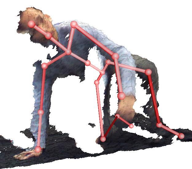
SMMC-10                 EVAL                    PDT
Subjects    One male          Two males, one         Three males, one
                                                                                Parameters: The parameters in our algorithm are empiri-
                              female                 female                     cally set to fixed values throughout our experiments and are
Data size 28 Sequences, 100 7 sequences per          4 sequences per            listed in Table 1. The only exception is the u in Eq. 1, which
           or 400 frames each subject, around 500    subject, 1000~2000
           (~50% each case) frames per sequence      frames per sequence        denotes the degree of noise and is data dependent. It is set
Motion     Relatively simple  Moderate to complex    Moderate to complex        to 0.01 unless significant noises are present. Although in
complexity                    (cart-wheels, hand     (jumping, sitting on
                              standing, sitting on   floor, dancing, etc.)
                                                                                other related methods[19, 6], σ 2 is initialized from the input
                              floor, etc.)                                      data directly, we found that such strategy generally largely
Ground     Markers            Joints                 Joints + Transformations   overestimates the value of σ 2 and will try to collapse the
truth data
                                                                                template to fit the input point cloud. Different from shape
Figure 3. The three datasets we use for quantitative evaluations.               registration applications, for articulated shapes tracking, it
                                                                                would destroy the temporal information and introduce extra
between connected vertex pairs. In our implementation, we
                                                                                ambiguities. Therefore we use a fixed value instead. Due to
prune correspondences based on euclidean distance in each
                                                                                the multiplier σ12 in Eq. 13, which is normally ≥ 104 , the
frame to remove noises, and perform this adaptation only
                                                                                regularization terms generally require large global weights.
every L (L = 5 in our experiments) frames because nearby
frames in general provide little new information.                                                               Eq. 20              Eq. 27          Eq. 30
                                                                                          Initial σ 2          λr     λp             λs            λd λe
3.5.3      Template Initialization
                                                                                         0.022 (m2 )          1000 500              1000           1 0.1
As opposed to most existing methods that require prior                                   Table 1. The parameter settings for our experiments.
knowledge of initial pose, our method can handle large pose
variations. In general, our tracker only requires knowledge                     4.1. Tracking Accuracy Evaluations
of the rough global orientation of the subject, for example,
whether the subject is facing towards the camera or to the                          The accuracy of our algorithm is evaluated on three pub-
left, etc. The local configuration of each limb can be effec-                   licly available datasets, namely SMMC-10 [11], EVAL [12]
tively derived using our tracking algorithm in most cases.                      and PDT [13], that contain ground truth joint (marker) lo-
Please see our supplemental materials for examples. For                         cations. A summary of these datasets is provided in Fig. 3.
pose tracking applications, the limb length estimation pro-                     Due to the discrepancy of ground truth data format provided
cess described in Sec. 3.5.1 is performed using the first F                     and joint definitions across trackers, different methods for
frames (F = 5 in our experiments), as it requires repeated                      accuracy measurement are needed. For the SMMC-10 and
pose estimation and is relatively more time-consuming. No-                      EVAL datasets, we use the same strategy as in [30]. Specif-
tice that the algorithm favors all segments of the articulated                  ically, we align our template to one single frame and mount
object being visible, as the scales of the invisible parts can                  the corresponding markers to our template. The markers are
only be estimated via the regularization term in Eq. 27 and                     then transformed with our estimated pose and directly com-
might not be accurate. In addition, poses that resolves more                    pared with the ground truth. For the PDT dataset, we follow
joint ambiguities are preferred in this process. For example,                   the strategy described in their paper [13]. The estimated
an arm bending pose better defines the length of both the                       joints are transformed via the provided transformations to
upper arm and forearm than a T-pose.                                                        Articulated ICP       Ganapathi et al. [11]   Shotton et al. [24]
                                                                                            Wei et al. [28]       Ganapathi et al. [12]   Ours
                                                                                   1
4. Experiments                                                                  0.95
                                                                                 0.9
                                                                                0.85
                                                                                 0.8
    In order to take advantage of the parallelism of the com-                   0.75
                                                                                 0.7
putations in our algorithm, especially the calculation of pos-
teriors, we implement our pipeline on GPU with CUDA.
With our current un-optimized implementation, each iter-
                                                                                                 (a) Comparison in terms of prediction precision
ation of our pose estimation together with geometric shape
                                                                                 0.08
adaptation takes about 1.5ms on average, with sub-sampling                       0.06
of around 1000 points for each point set. The running time                       0.04
                                                                                 0.02
is measured on a machine with Intel Core i7 3.4GHz CPU                                    Ganapathi et   Ye et al. [31] Baak et al. [1] Helten et al.       Ours
and Geforce GTX 560 Ti graphics card. Since our algo-                                       al. [11]                                        [14]
rithm normally requires < 15 iterations in total to converge                            (b) Comparison in terms of marker distance errors (unit = meter)
during tracking, the entire pipeline runs at real time. In our                  Figure 4. Quantitative evaluation of our tracker on the SMMC-10
experiments, we assume segmentation of the target subject                       dataset [11] with two error metrics. Notice that in (b), although
is relatively simple using depth information. Therefore, the                    the method by Ye et al. [30] achieves comparative accuracy, their
computational time for segmentation is not considered here.                     reported computation time is much higher.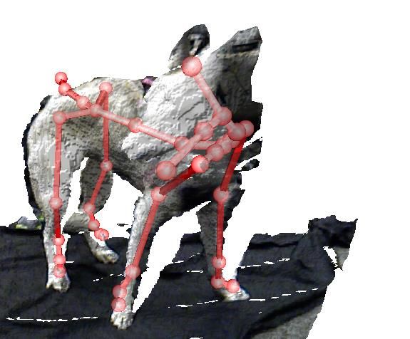
0.95 0.1
0.9
0.85 0.08
0.8 0.06
0.75
0.7 0.04
Articulated Ganapathi et Ours KinectSDK Baak et Helten et Ours
ICP al. [12] [17] al. [1] al. [14]
(a) Comparison of prediction (b) Comparison of joint distance errors
precision on EVAL dataset (unit = meter) on PDT dataset
EVAL PDT
1 Figure 8. Example results of our algorithm applied to dog data.
0.95
0.9
0.85
0.8
0.75
0.7
Non-human Subjects Our algorithm can also be applied
to articulated objects other than human beings. To demon-
strate its applicability, we test on data captured from a dog.
(c) Our prediction precision on the EVAL and PDT dataset
A major challenge in this data is the severe self occlusions.
Figure 5. Quantitative evaluations of our tracker’s accuracy with Some of our results are show in Fig. 1 and Fig. 8. Note that
comparisons with the state of the arts. for discriminative and hybrid approaches, a database of this
local coordinate system of each corresponding joint, and the animal will be needed; while we only need a skinning tem-
mean of displacement vectors for each joint is subtracted to plate. Besides, none of existing generative methods have
account for joint definition difference. reported results on this type of data, except with multi-view
Previous methods reported their accuracy according to setup that resolves the severe occlusion [10].
two different error metrics, directly measurement of the eu-
clidean distance between estimated and ground truth joints, 4.2. Shape Adaptation Accuracy
or the percentage of correctly estimated joints (euclidean
To quantitatively evaluate the performance of our body
distance error within 0.1m). Therefore, we show our re-
shape adaptation algorithm, we compare our results on the
sults in both ways for comparison purpose. The accuracy
PDT dataset [13] with their ground truth shape data. Note
of our tracker on the SMMC-10 dataset is shown in Fig. 4.
that in our pipeline, the body shapes are automatically de-
In this relatively simple dataset, our method outperforms
duced during the tracking process, while a specific calibra-
most existing methods, and is comparable with two recent
tion procedure is required in [13]. To measure fitting errors,
work [12, 27]. The comparisons on the other two more chal-
we estimate the pose of the ground truth shape using our
lenging datasets are shown in Fig. 5. The results clearly
algorithm and deform our template accordingly. On aver-
show that our method outperforms all the compared meth-
age, we achieve comparative accuracy as Heltel et al. [13]:
ods by a large margin. That means our approaches can han-
0.012m v.s 0.010m. To compare, the mean fitting error re-
dle complex motions more accurately and robustly, while
ported by Weiss et al. [28] on their own test data is around
still achieves real-time performance. (The numbers for the
0.010m. It should be emphasized that [13] requires an ex-
compared methods are reproduced from their own papers,
tra calibration procedure and [28] assumes small motion be-
except for the Articulated ICP and the KinectSDK of which
tween their input, while our method directly operates on the
the numbers are obtained from [12] and [13], respectively.)
dynamic input. It should also be pointed out that the ground
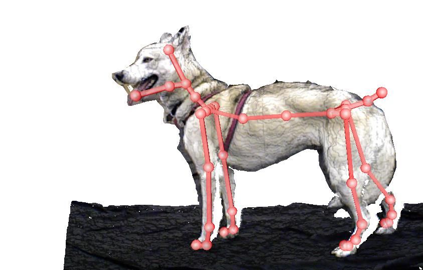
As mentioned before, our tracker well handles complex truth shapes from [13] were obtained by fitting SCAPE
motions. The tracking results of various complex poses models to data from scanner. Thus they do not well cap-
from our own data and the publicly available datasets are ture the effects of subject’s clothing, which is captured by
shown in Fig. 1 and in Fig. 6 respectively. Furthermore, vi- our algorithm through fitting with the input data. In Fig. 9,
sual comparisons between our results and the skeletons es- the effectiveness of our adaptation procedure is visualized.
timated by KinectSDK are shown in Fig. 7. (More results
are provided in our supplemental materials.)
(a) (b) (c) (d)
Figure 9. Visual results of our shape adaptation algorithm. (a) and
(c) are results of only pose estimation (male and female respec-
tively), while (b) and (d) are results with shape adaptation during
tracking. Input meshes are overlaid on each result. Notice the
Figure 7. Visual comparison of our results (second row) with adjustment of limb lengths, in particular the arms and feet of the
KinectSDK [16] (first row) on some relatively complex poses. male subject.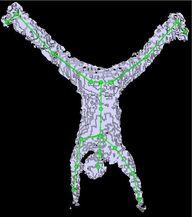
Figure 6. Visualization of example tracking results on the publicly available datasets.
5. Conclusion and Future Work                                                 [10] J. Gall, C. Stoll, E. de Aguiar, C. Theobalt, B. Rosenhahn, and H.-
                                                                                   P. Seidel. Motion capture using joint skeleton tracking and surface
   In this paper, we proposed a novel algorithm for simulta-                       estimation. In CVPR. IEEE, 2009.
neous pose and shape estimation for articulated objects us-                   [11] V. Ganapathi, C. Plagemann, D. Koller, and S. Thrun. Real time
                                                                                   motion capture using a single time-of-flight camera. In CVPR, 2010.
ing one single depth camera. Our pipeline is fully automatic
                                                                              [12] V. Ganapathi, C. Plagemann, D. Koller, and S. Thrun. Real-time
and runs in real time. Through extensive experiments, we                           human pose tracking from range data. In ECCV, 2012.
have demonstrated the effectiveness of our algorithm, espe-                   [13] T. Helten, A. Baak, G. Bharaj, M. Müller, H.-P. Seidel, and
cially in handling complex motions. In particular, we have                         C. Theobalt. Personalization and evaluation of a real-time depth-
shown results of tracking an animal, which have not been                           based full body tracker. In 3DV, 2013.
                                                                              [14] H. Li, L. Luo, D. Vlasic, P. Peers, J. Popović, M. Pauly, and
demonstrated in previous methods with monocular setup.                             S. Rusinkiewicz. Temporally coherent completion of dynamic
   Our pose tracker could be further improved, for example                         shapes. ACM TOG, 31(1):2:1–2:11, Feb. 2012.
by taking into account free space constraints as in [12]. Be-                 [15] H. Li, E. Vouga, A. Gudym, L. Luo, J. T. Barron, and G. Gusev. 3d
sides, the computational complexity can be greatly reduced                         self-portraits. SIGGRAPH ASIA, 32(6), November 2013.
                                                                              [16] Microsoft.       Kinectsdk.      http://www.microsoft.com/
through fast Gauss transform during computation of the                             en-us/kinectforwindows/, 2013.
posteriors [19]. Looking into the future, we would like to                    [17] T. B. Moeslund, A. Hilton, and V. Krüger. A survey of advances in
explore schemes for adaptive limb lengths estimation along                         vision-based human motion capture and analysis. CVIU, 2006.
with pose estimation, instead of simply using the first few                   [18] R. M. Murray, S. S. Sastry, and L. Zexiang. A Mathematical Intro-
                                                                                   duction to Robotic Manipulation. CRC Press, Inc., Boca Raton, FL,
frames, which usually does not provide complete desired
                                                                                   USA, 1st edition, 1994.
information. Besides, with dynamic scenes, similar to most                    [19] A. Myronenko and X. B. Song. Point-set registration: Coherent point
existing techniques, our method only captures the subject’s                        drift. TPAMI, 2010.
overall shape. The challenging problem of reconstructing                      [20] C. Plagemann, V. Ganapathi, D. Koller, and S. Thrun. Real-time
detailed geometry is also interesting.                                             identification and localization of body parts from depth images. In
                                                                                   ICRA, pages 3108–3113, 2010.
                                                                              [21] G. Pons-Moll, J. Taylor, J. Shotton, A. Hertzmann, and A. Fitzgib-
Acknowledgments This work is supported in part by                                  bon. Metric regression forests for human pose estimation. In BMVC,
US National Science Foundation grants IIS-1231545 and                              2013.
IIS-1208420 , and Natural Science Foundation of China                         [22] R. Poppe. Vision-based human motion analysis: An overview. CVIU,
(No.61173105,61373085, 61332017).                                                  108(1-2):4–18, Oct. 2007.
                                                                              [23] J. Shotton, A. Fitzgibbon, M. Cook, T. Sharp, M. Finocchio,
References                                                                         R. Moore, A. Kipman, and A. Blake. Real-time human pose recog-
                                                                                   nition in parts from single depth images. In CVPR, 2011.
 [1] A. Baak, M. Müller, G. Bharaj, H.-P. Seidel, and C. Theobalt. A data-   [24] M. Straka, S. Hauswiesner, M. Rüther, and H. Bischof. Simultaneous
     driven approach for real-time full body pose reconstruction from a            shape and pose adaption of articulated models using linear optimiza-
     depth camera. In ICCV, pages 1092–1099. IEEE, Nov. 2011.                      tion. In ECCV, volume 7572, pages 724–737. 2012.
 [2] C. Bregler, J. Malik, and K. Pullen. Twist based acquisition and         [25] J. Taylor, J. Shotton, T. Sharp, and A. Fitzgibbon. The vitruvian
     tracking of animal and human kinematics. IJCV, 2004.                          manifold: Inferring dense correspondences for one-shot human pose
 [3] B. J. Brown and S. Rusinkiewicz. Global non-rigid alignment of 3-d            estimation. In CVPR, 2012.
     scans. In SIGGRAPH). ACM, 2007.                                          [26] D. Vlasic, I. Baran, W. Matusik, and J. Popović. Articulated mesh
 [4] W. Chang and M. Zwicker. Global registration of dynamic range                 animation from multi-view silhouettes. In SIGGRAPH), pages 97:1–
     scans for articulated model reconstruction. ACM TOG, 2011.                    97:9. ACM, 2008.
 [5] Y. Cui, W. Chang, T. Nöll, and D. Stricker. Kinectavatar: Fully auto-   [27] X. Wei, P. Zhang, and J. Chai. Accurate realtime full-body motion
     matic body capture using a single kinect. In ACCV 2012 Workshop               capture using a single depth camera. SIGGRAPH ASIA, 31(6):188:1–
     on Color Depth Fusion in Computer Vision, Nov 2012.                           188:12, Nov. 2012.
 [6] Y. Cui, S. Schuon, S. Thrun, D. Stricker, and C. Theobalt. Algorithms    [28] A. Weiss, D. Hirshberg, and M. J. Black. Home 3d body scans from
     for 3d shape scanning with a depth camera. TPAMI, PP(99):1, 2012.             noisy image and range data. In ICCV. IEEE, 2011.
 [7] E. de Aguiar, C. Stoll, C. Theobalt, N. Ahmed, H.-P. Seidel, and         [29] G. Ye, Y. Liu, N. Hasler, X. Ji, Q. Dai, and C. Theobalt. Performance
     S. Thrun. Performance capture from sparse multi-view video. ACM               capture of interacting characters with handheld kinects. In ECCV,
     TOG, 2008.                                                                    pages 828–841, 2012.
 [8] A. P. Dempster, N. M. Laird, and D. B. Rubin. Maximum likelihood         [30] M. Ye, X. Wang, R. Yang, L. Ren, and M. Pollefeys. Accurate 3d
     from incomplete data via the EM algorithm. Journal of the Royal               pose estimation from a single depth image. In ICCV, 2011.
     Statistical Society, 39:1–38, 1977.
                                                                              [31] M. Zeng, J. Zheng, X. Cheng, and X. Liu. Templateless quasi-rigid
 [9] J. Gall, A. Fossati, and L. Van Gool. Functional categorization of            shape modeling with implicit loop-closure. In CVPR, June 2013.
     objects using real-time markerless motion capture. In CVPR, 2011.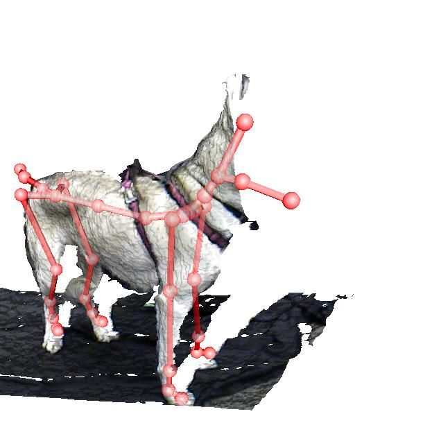
You can also read