Learning Spatio-Temporal Structure from RGB-D Videos for Human Activity Detection and Anticipation
←
→
Page content transcription
If your browser does not render page correctly, please read the page content below
Learning Spatio-Temporal Structure from RGB-D Videos for
              Human Activity Detection and Anticipation

Hema S. Koppula                                                                       hema@cs.cornell.edu
Ashutosh Saxena                                                                    asaxena@cs.cornell.edu
Computer Science Department, Cornell University, Ithaca, NY 14853 USA

                     Abstract                              searchers to model such rich spatio-temporal interac-
                                                           tions in the 3D scene for learning complex human ac-
    We consider the problem of detecting past
                                                           tivities. For example, Koppula, Gupta and Saxena
    activities as well as anticipating which activ-
                                                           (2013) (KGS) used a conditional random field (CRF),
    ity will happen in the future and how. We
                                                           trained with max-margin methods, to model the rich
    start by modeling the rich spatio-temporal
                                                           spatio-temporal relations between the objects and hu-
    relations between human poses and objects
                                                           mans in the scene.
    (called affordances) using a conditional ran-
    dom field (CRF). However, because of the               However, in previous works, emphasis has been on
    ambiguity in the temporal segmentation of              modeling the relations between components in the
    the sub-activities that constitute an activity,        scene (human pose, objects, etc.), and performing
    in the past as well as in the future, mul-             learning and inference given the spatio-temporal struc-
    tiple graph structures are possible. In this           ture of the model (i.e., for a given CRF structure in
    paper, we reason about these alternate pos-            the case of KGS). However, it is quite challenging to
    sibilities by reasoning over multiple possi-           estimate this structure because of two reasons. First,
    ble graph structures. We obtain them by                an activity comprises several sub-activities, of vary-
    approximating the graph with only additive             ing temporal length, performed in a sequence. This
    features, which lends to efficient dynamic             results in an ambiguity in the temporal segmentation
    programming. Starting with this proposal               and thus a single graph structure may not explain the
    graph structure, we then design moves to               activity well. Second, there can be several possible
    obtain several other likely graph structures.          graph structures when we are reasoning about activi-
    We then show that our approach improves                ties in the future (i.e., when the goal is to anticipate
    the state-of-the-art significantly for detecting       future activities, different from just detecting the past
    past activities as well as for anticipating fu-        activities). Multiple spatio-temporal graphs are possi-
    ture activities, on a dataset of 120 activity          ble in these cases and we need to reason over them in
    videos collected from four subjects.                   our learning algorithm.
                                                           In our work, we start by using a CRF to model the
                                                           sub-activities and affordances of the objects, how they
1. Introduction                                            change over time, and how they relate to each other.
Being able to detect which activity is being performed     In detail, we have two kinds of nodes: object and sub-
as well as being able to anticipate what is going to       activity nodes. The edges in the graph model the pair-
happen next in an environment is important for ap-         wise relations among interacting nodes, namely the
plication domains such as robotics and surveillance.       object–object interactions, object–sub-activity inter-
In a typical environment, we have humans interact-         actions, and the temporal interactions (see Figure 1).
ing with the objects and performing a sequence of ac-      This model is built with each spatio-temporal segment
tivities. Recently, inexpensive RGB-D cameras (such        being a node. Figure 2 shows two possible graph struc-
as Microsoft Kinect, see Figure 1) have enabled re-        tures for an activity with two objects. We then reason
                                                           about the possible graph structures for both past and
Proceedings of the 30 th International Conference on Ma-   future activities. The key idea is to first sample a few
chine Learning, Atlanta, Georgia, USA, 2013. JMLR:         segmentations that are close to the ground-truth seg-
W&CP volume 28. Copyright 2013 by the author(s).           mentation using our CRF model instantiated with a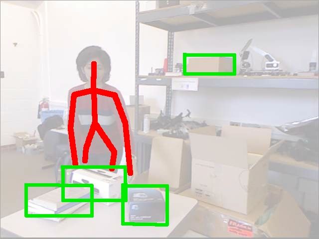
Learning Spatio-Temporal Structure from RGB-D Videos for Human Activity Detection & Anticipation
!"#$%&'()*+,-'./01!2))
13!"&'./%3*)4''5)
past frames future frames
*$'/'()%,6".!)7)*+,-'./01!2)
13!"&'./%3*)4%'5)
*$'/'()%,6".!-)%,6".!)
13!"&'./%3*)4%%5)
!"#$%&'()%,6".!)-)%,6".!)
13!"&'./%3*)4%%5)
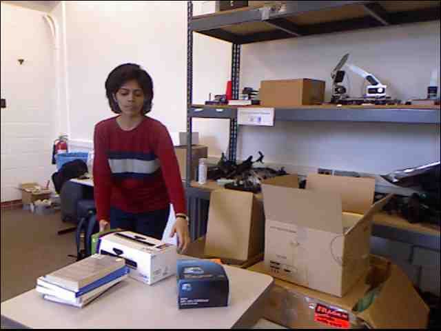
Figure 1. An example activity from the CAD-120 dataset
(top row) and one possible graph structure (bottom row).
Top row shows the RGB image (left), depths (middle),
and the extracted skeleton and object information (right).
(Graph in the bottom row shows the nodes at only the tem- past frames future frames
poral segment level, the frame level nodes are not shown.) Figure 2. Figure illustrating two possible graph structures
(top and bottom), with six observed frames in the past
subset of features, and then explore the space of seg- and three anticipated frames in the future. This example
mentation by making merge and split moves to create has one sub-activity node and two object nodes in each
temporal segment.
new segmentations. We do so by approximating the
graph with only additive features, which lends to effi-
Ly et al., 2012). This, together with depth infor-
cient dynamic programming.
mation, has enabled some recent works (Sung et al.,
In extensive experiments over 120 activity videos col- 2011; Zhang & Parker, 2011; Ni et al., 2011; Sung
lected from four subjects, we showed that our ap- et al., 2012) to obtain good action recognition perfor-
proach outperforms the state-of-the-art results both mance. However, these methods only address detec-
in the tasks of activity and affordance detection. We tion over small periods of time, where temporal seg-
achieved an accuracy of 85.4% for affordance, 70.3% mentation (and thus knowledge of the spatio-temporal
for sub-activity labeling and 83.1% for high-level ac- graph structure) is not a big problem. KGS (Kop-
tivities respectively for detection. Furthermore, we pula et al., 2013) proposed a model to jointly predict
obtain an accuracy of 67.2% and 49.6% for anticipat- sub-activities and object affordances by taking into ac-
ing affordances and sub-activities respectively in fu- count both spatio-temporal interactions between hu-
ture time-frames. man poses and objects over longer time periods. How-
ever, KGS found that not knowing the graph structure
2. Related Work (i.e., the correct temporal segmentation) decreased the
There has been a considerable amount of previous performance significantly. This is because the bound-
work on detection of human activities from still im- ary between two sub-activities is often not very clear,
ages as well as videos (e.g., Maji et al., 2011; Yang as people often start performing the next sub-activity
et al., 2010; Xing et al., 2008; Ryoo, 2011; Hoai & De before finishing the current sub-activity. We compare
la Torre, 2012a). Similar to our setting some recent our proposed method with theirs and show consider-
works have shown that modeling the mutual context able improvement over their state-of-the-art results.
between human poses and objects (either the category
In activity detection from 2D videos, much previous
label or affordance label, Jiang et al. 2012a) is use-
work has focussed on short video clips, assuming that
ful for activity detection (Gupta et al., 2009; Yao &
temporal segmentation has been done apriori. Some
Fei-Fei, 2010; Delaitre et al., 2011; Prest et al., 2012;
recent effort in recognizing actions from longer video
Koppula et al., 2013).
sequences take an event detection approach (Ke et al.,
Recent availability of inexpensive RGB-D sensors has 2007; Simon et al., 2010; Nguyen et al., 2009), where
enabled significant improvement in scene modeling they evaluate a classifier function at many different
(Koppula et al., 2011; Anand et al., 2012; Jiang et al., segments of the video and then predict the event pres-
2012b; 2013; Jia et al., 2013; Jiang & Saxena, 2013) ence in segments. Similarly, change point detection
and estimation of human poses (Shotton et al., 2012; methods (Xuan & Murphy, 2007; Harchaoui et al.,Learning Spatio-Temporal Structure from RGB-D Videos for Human Activity Detection & Anticipation
2008) work by performing a sequence of change-point works maintain their template graph structure over
analysis in a sliding window along the time dimension. time, in our work, new graph structures are possible.
However, these methods only detect local boundaries Works on semi-Markov models (Sarawagi & Cohen,
and tend to over-segment complex actions which often 2004; Shi et al., 2011) are quite related to our work
contain many changes in local motion statistics. as they address the problem of finding the segmenta-
tion along with labeling. However, these methods are
Some previous works consider joint segmentation and
limited since they are only efficient for feature maps
recognition by defining dynamical models based on
that are additive in nature. We build upon these ideas
kinematics (Oh et al., 2008; Fox et al., 2009), but these
where we use the additive feature map as only a close
works do not model the complex human-object inter-
approximation to the graph structure and then explore
actions. Hoai et al. (2011) and Hoai & De la Torre
the space of likely graph structure by designing moves.
(2012b) do not consider temporal context and only
We show that this improves performance while being
perform activity classification and clustering respec-
computationally efficient.
tively. In related work, Ion et al. (2011) consider the
problem 2D image segmentation. They sample seg- 3. Modeling Spatio-Temporal Relations
mentations of images for labeling using an Incremen-
for a Given Graph Structure
tal Saddle Point estimation procedure which require
good initial samples. In contrast, our application re- In our setting, our algorithm observes a scene contain-
quires modeling of the temporal context (as compared ing a human and objects for time t in the past, and our
to just spatial). This work is closer to KGS, where they goal is to detect activities in the observed past and also
also sample the segmentation space. However, in our anticipate the future activities for time d. Following
approach we use a discriminative approach, where we KGS, we discretize time to the frames of the video1 and
model the energy function as composed of an additive group the frames into temporal segments, where each
and a non-additive term. This allows us to efficiently temporal segment spans a set of contiguous frames cor-
sample the potential graph structures. responding to a single sub-activity. Therefore, at time
‘t’ we have observed ‘t’ frames of the activity that are
One important application of our approach is in antic- grouped into ‘k’ temporal segments. (Figure 2 shows
ipating future activities, where reasoning over future two temporal segments for the past.)
possible graph structures becomes important. Antic-
ipating future activities has gained attention only re- We model the spatio-temporal structure of an activity
cently (Kitani et al., 2012; Koppula & Saxena, 2013). using a conditional random field, illustrated in Fig-
Kitani et al. (2012) proposed a Markov decision pro- ure 1. For the past t frames, we know the nodes of
cess to obtain a distribution over possible human navi- the CRF but we do not know the temporal segmen-
gation trajectories in 2D from visual data. Koppula & tation, i.e., which frame level nodes are connected to
Saxena (2013) addressed the problem of anticipating each of the segment level node. The node labels are
human activities at a fine-grained level of how humans also unknown. For the future d frames, we do not even
interact with objects in more complex activities such know the nodes in the graph—there maybe different
as microwaving food or taking medicine. They repre- number of objects being interacted with depending on
sent the distribution of the possible futures with a set which sub-activity is performed in the future. Our goal
of particles that are obtained by augmenting the CRF is to explore different possible past and future graph
structure of KGS with sampled future nodes. However, structures (i.e., sub-activities, human poses, object lo-
they do not reason about the possible graph structures cations and affordances). We will do so by augment-
for the past. In our work, we show that sampling the ing the graph in time with potential object nodes, and
spatio-temporal structure, in addition to sampling the sampling several possible graph structures.
future nodes, results in better anticipation. We first describe the CRF modeling given a fixed
In terms of learning algorithms, probabilistic graphical graph structure for t observed frames. Let, s ∈
models are a workhorse of machine learning and have {1, .., N } denote a temporal segment and y =
been applied to a variety of applications. Frameworks (y1 , ..., yN ) denote the labeling we are interested in
such as HMMs (Hongeng & Nevatia, 2003; Natarajan finding, where ys is the set of sub-activity and ob-
& Nevatia, 2007), DBNs (Gong & Xiang, 2003), CRFs ject affordance labels for the temporal segment s. Our
(Quattoni et al., 2007; Sminchisescu et al., 2005; Kop- input is a set of features Φ(x) extracted from the seg-
pula et al., 2013), and semi-CRFs (Sarawagi & Cohen, 1
In the following, we will use the number of videos
2004) have been previously used to model the tempo- frames as a unit of time, where 1 unit of time ≈ 71ms
ral structure of videos and text. While most previous (=1/14, for a frame-rate of about 14Hz).Learning Spatio-Temporal Structure from RGB-D Videos for Human Activity Detection & Anticipation
mented 3D video. The prediction ŷ is computed as satisfy this property are referred to as the non-additive
the argmax of an energy function E(y|Φ(x); w) that features, for example, maximum and minimum dis-
is parameterized by weights w. tances between two objects. As we discuss in the next
section, additive features allow efficient joint segmen-
ŷ = argmax E(y|Φ(x); w) (1) tation and labeling by using dynamic programming,
y
but may not be expressive enough.
This energy is expressed over a graph, G = (V, E) (as il-
lustrated in Figure 1), and consists of two terms—node Non-additive features sometimes provide very useful
terms and edge terms. Each of these terms comprises cues for discriminating the sub-activity and affordance
the label, appropriate features, and weights. Let yik be classes. For example, consider discriminating cleaning
a binary variable representing the node i having label sub-activity from a moving sub-activity: here the total
k, where K is the set of labels. Let φn (i) and φe (i, j) distance moved could be similar (an additive feature),
be the node and edge feature maps respectively. (De- however, the minimum and maximum distance moved
pending on the node and edge being used, the appro- being small may be strong indicator of the activity be-
priate subset of features and class labels are used.) We ing cleaning. In fact, when compared to our model
thus write the energy function as: learned using only the additive features, the model
XX h i learned with both additive and non-additive features
E(y|Φ(x); w) = yik wnk · φn (i) , improves macro precision and recall by 5% and 10.1%
i∈V k∈K
h i for labeling object affordance respectively and by 3.7%
X X
+ yil yjk welk · φe (i, j) (2) and 6.2% for labeling sub-activities respectively.
(i,j)∈E (l,k)∈K×K
In detail, we use the same features as described by
Note that the graph has two types of nodes: sub- KGS. These features include the node feature maps
activity and object nodes, and it has four types of φo (i) and φa (j) for object node i and sub-activity node
edges: object–object edges, object–sub-activity edges, j respectively, and edge feature maps φt (i, j) capturing
object–object temporal edges, and sub-activity–sub- the relations between various nodes. The object node
activity temporal edges. Our energy function is a sum feature map, φo (i), includes the (x, y, z) coordinates of
of six types of potentials that define the energy of a the object’s centroid, the coordinates of the object’s
particular assignment of sub-activity and object affor- bounding box and transformation matrix w.r.t. to the
dance labels to the sequence of segments in the given previous frame computed at the middle frame of the
video: E(y|Φ(x); w) = Eo +Ea +Eoo +Eoa +Eoo t
+Eaat
. temporal segment, the total displacement and the to-
However, we have written it compactly in Eq. (2). tal distance moved by the object’s centroid in the set
of frames belonging to the temporal segment. The
Learning and Inference. As the structure of the sub-activity node feature map, φa (j), gives a vector
graph is fully known, we learn the parameters of the of features computed using the noisy human skeleton
energy function in Eq. (2) by using the cutting plane poses obtained from running Openni’s skeleton tracker
method (Joachims et al., 2009). on the RGBD video. We compute the above described
However, during inference we only know the nodes in location (relative to the subject’s head location) and
the graph but not the temporal segmentation, i.e., the distance features for each the upper-skeleton joints ex-
structure of the graph in terms of the edges connecting cluding the elbow joints (neck, torso, left shoulder, left
frame level nodes to the segment level label nodes. palm, right shoulder and right palm).
We could search for the best labeling over all possible The edge feature maps, φt (i, j), include relative geo-
segmentations, but this is very intractable because our metric features such as the difference in (x, y, z) coor-
feature maps contain non-additive features (that are dinates of the object centroids and skeleton joint lo-
important and are described in the next sub-section). cations and the distance between them. In addition
to computing these values at the first, middle and last
3.1. Features: Additive and Non-Additive frames of the temporal segment, we also consider the
We categorize the features into two sets: additive fea- min and max of their values across all frames in the
tures, ΦA (x), and non-additive features, ΦN A (x). We temporal segment to capture the relative motion in-
compute the additive features for a set of frames cor- formation. The temporal relational features capture
responding to a temporal segment by adding the fea- the change across temporal segments and we use the
ture values for the frames belonging to the temporal vertical change in position and the distance between
segment. Examples of the additive features include corresponding object and joint locations. We perform
distance moved and vertical displacement of an object cumulative binning of all the feature values into 10
within a temporal segment. The features that do not bins for each feature.Learning Spatio-Temporal Structure from RGB-D Videos for Human Activity Detection & Anticipation
4. Sampling Spatio-Temporal Graphs Heuristic Segmentations. There is a lot of infor-
mation present in the video which can be utilized for
Efficient Inference with Additive Features. We the purpose of temporal segmentation. For example,
express the feature set, Φ(x), as the concatenation of smooth movement of the skeleton joints usually rep-
the additive and non-additive feature sets, ΦA (x) and resent a single sub-activity and the sudden changes in
ΦN A (x) respectively. Therefore, by rearranging the the direction or speed of motion indicate sub-activity
terms in Eq. (2), the energy function can written as: boundaries. Therefore, we incorporate such informa-
tion in performing temporal segmentation of the activ-
E(y|Φ(x); w) = E(y|ΦA (x); w) + E(y|ΦN A (x); w) ities. In detail, we use the multiple segmentation hy-
potheses proposed by KGS. These include graph based
We perform efficient inference for the energy term segmentation method proposed by (Felzenszwalb &
E(y|ΦA (x); w) by formulating it as a dynamic pro- Huttenlocher, 2004) adapted to temporally segment
gram (see Eq. (3)). In detail, let L denote the max the videos. The sum of the Euclidean distances be-
length of a temporal segment, i denote the frame in- tween the skeleton joints and the rate of change of
dex, s denote the temporal segment spanning frames the Euclidean distance are used as the edge weights
(i − l) to i, and (s − 1) denote the previous segment. for two heuristic segmentations respectively. By vary-
We write the energy function in a recursive form as: ing the thresholds, different temporal segmentations
X h i of the given activity can be obtained. In addition to
V (i, k) = 0
max V (i − l, k0 ) + ysk wnk · φA
n (s) the graph based segmentation methods, we also use
k ,l=1...L
k∈K
X h i the uniform segmentation method which considers a
+ ysk welk · φA
e (s − 1, s) (3) set of continuous frames of fixed size as the temporal
k∈K segment. There are two parameters for this method:
the segment size and the offset (the size of the first seg-
Here, φA A
n (s) and φe (s − 1, s) denote the additive fea-
ment). However, these methods often over-segment a
ture maps and can be efficiently computed by using the sub-activity, and each segmentation would result in a
concept of integral images.2 The best segmentation different graph structure for our CRF modeling.
then corresponds to the path traced by maxa V (t, a), We generate multiple graph structures for various val-
where t is the number of video frames. ues of the parameters for the above mentioned meth-
Using E(y|ΦA (x); w), we find the top-k scored seg- ods and obtain the predicted labels for each using
mentations and then evaluate them using the full Eq. (1). We obtain the final labeling over the segments
model E(y|Φ(x); w) in order to obtain more accurate by either using the second-step learning method pre-
labelings. sented in KGS, or by performing voting and taking
the label predicted by majority of the sampled graph
Merge and Split Moves. The segmentations structures (our experiments follow the latter).
generated by the approximate energy function,
E(y|ΦA (x); w), are often very close to the given
4.1. Anticipating and Sampling Future Nodes
ground-truth segmentations. However, since the en-
ergy function used is only approximate, it sometimes For anticipating the next d time, we augment the CRF
tends to over-segment or miss the boundary by a few structure with d frame nodes as proposed in (Kop-
frames. In order to obtain a representative set of seg- pula & Saxena, 2013). Sampling this graph comprises
mentation samples, we also perform random merge three steps. First, we need to sample the possible sub-
and split moves over these segmentations, and con- activity and the object nodes involved. Second, for
sider them for evaluating with the full model as well. this segment-level graph, we sample the frame-level
A merge move randomly selects a boundary and re- nodes, starting with possible end-points of the physi-
moves it, and a split move randomly chooses a frame cal location of the objects and human hands. Third,
in a segment and creates a boundary. given the end locations, we sample a variety of tra-
2 jectories. This sampling procedure gives us various
The additive features for temporal segments starting at
the first frame and ending at frame l, for l = 1..t are pre- possible future nodes and their spatial relations. We
computed, i.e., the segment features for a total of t tempo- add these to the observed nodes and sample various
ral segments are computed. This needs (n×t) summations, possible temporal segmentations as described above.
where n is the number of features. Now the segment fea-
tures for a temporal temporal segment starting and ending In the first step, we sample the object affordances and
at any frame can be computed by n subtractions. There- activities based on a discrete distribution generated
fore, the total feature computation cost is linear in the from the training data. This distribution is based on
number of possible segmentations.Learning Spatio-Temporal Structure from RGB-D Videos for Human Activity Detection & Anticipation
the object type (e.g., cup, bowl, etc.) and object’s cur- 5. Experiments
rent position with respect to the human in the scene Data. We test our model on the Cornell Activity
(e.g., in contact with the human hand, etc.). For ex- Dataset-120 (CAD-120) (Koppula et al., 2013). It con-
ample, if a human is holding an object of type ‘cup’ tains 120 3D videos of four different subjects perform-
placed on the table, then the affordances drinkable ing 10 high-level activities, where each high-level activ-
and movable with their corresponding sub-activities ity was performed three times with different objects.
(drinking and moving respectively) have equal proba- It contains a total of 61,585 total 3D video frames. The
bility, with all others being 0. activities have a long sequence of sub-activities, which
In the second step, given the sampled affordances and vary from subject to subject significantly in terms of
sub-activity, we sample the corresponding object loca- length of the sub-activities, order of the sub-activities
tions and human poses for the d anticipated frames. as well as in the way they executed the task. The
In order to have meaningful object locations and hu- dataset is labeled with both sub-activity and object af-
man poses we take the following approach. We model fordance labels. The high-level activities are: {making
object affordances using a potential function based on cereal, taking medicine, stacking objects, unstacking
how the object is being interacted with, when the cor- objects, microwaving food, picking objects, cleaning ob-
responding affordance isQactive. The jects, taking food, arranging objects, having a meal }.
Q affordance poten- The sub-activity labels are: {reaching, moving, pour-
tial has the form ψo = i ψdisti j ψorij , where ψdisti
ing, eating, drinking, opening, placing, closing, scrub-
is the ith distance potential and ψorij is the j th relative
bing, null } and affordance labels are: {reachable, mov-
angular potential. We model each distance potential
able, pourable, pourto, containable, drinkable, openable,
with a Gaussian distribution and each relative angu-
placeable, closable, scrubbable, scrubber, stationary}.
lar potential with a von Mises distribution and find the
parameters from the training data. We can now score Evaluation: For comparison, we follow the same
the points in the 3D space using the potential function, train-test split described in KGS and train our model
whose value represents the strength of the particular on activities performed by three subjects and test on
affordance at that location. Therefore, for the chosen activities of a new subject. We report the results ob-
affordance, we sample the object’s most likely future tained by 4-fold cross validation by averaging across
location using the affordance potentials. the folds. We consider the overall micro accuracy
(P/R), macro precision and macro recall of the de-
In the third step, for every sampled target object
tected sub-activities, affordances and overall activity.
location, we generate a set possible trajectories fol-
Micro accuracy is the percentage of correctly classified
lowing which the object can be moved form its cur-
labels. Macro precision and recall are the averages of
rent location to the sampled target location. We
precision and recall respectively for all classes. We
use parametrized cubic equations, in particular Bézier
also computed these metrics for the anticipated sub-
curves, to generate human hand like motions (Faraway
activity and affordances.
et al., 2007). We estimate the control points of the
Bézier curves from the training data. Detection Results. Table 1 shows the performance
of our proposed approach on object affordance, sub-
Sampling Augmented Graphs. In order to sample
activity and high-level activity labeling for past activi-
the future graphs, we augment our observed frames
ties. Rows 3-5 show the performance for the case where
with these sampled future frames, and then sample
ground-truth temporal segmentation is provided and
the augmented graph structures (for different tempo-
rows 6-9 show the performance for the different meth-
ral segmentations) as described in Section 4. We then
ods when no temporal segmentation is provided. With
use the energy function in Eq. (2) to obtain the best
known graph structure, the model using the the full set
labeling for each sampled graph. The node potentials
of features (row 4) outperforms the model which uses
score how well the features extracted from the antici-
only the additive features (row 5): macro precision
pated object locations and human poses match the af-
and recall improve by 5% and 10.1% for labeling ob-
fordance and sub-activity labels respectively, and the
ject affordance respectively and by 3.7% and 6.2% for
edge potentials score how likely are the anticipated
labeling sub-activities respectively. This shows that
sub-activities and affordances likely to follow the ob-
additive features bring us close, but not quite, to the
served ones. Therefore, the value of the energy func-
optimal graph structure.
tion provides a ranking over the sampled augmented
graphs for the future time. For obtaining anticipa- When the graph structure is not known, the perfor-
tion metrics, we report the highest ranked one (and mance drops significantly. Our graph sampling ap-
compare it with what was actually performed in the proach based on the additive energy function (row 6)
future).Learning Spatio-Temporal Structure from RGB-D Videos for Human Activity Detection & Anticipation
Table 1. Results on CAD-120 dataset for detection, showing average micro precision/recall, and average macro
precision and recall for affordances, sub-activities and high-level activities. Computed from 4-fold cross validation with
testing on a new human subject in each fold. Standard error is also reported.
With ground-truth segmentation.
Object Affordance Sub-activity High-level Activity
micro macro micro macro micro macro
method P/R Prec. Recall P/R Prec. Recall P/R Prec. Recall
chance 8.3 (0.0) 8.3 (0.0) 8.3 (0.0) 10.0 (0.0) 10.0 (0.0) 10.0 (0.0) 10.0 (0.0) 10.0 (0.0) 10.0 (0.0)
max class 65.7 (1.0) 65.7 (1.0) 8.3 (0.0) 29.2 (0.2) 29.2 (0.2) 10.0 (0.0) 10.0 (0.0) 10.0 (0.0) 10.0 (0.0)
KGS (Koppula et al., 2013) 91.8 (0.4) 90.4 (2.5) 74.2 (3.1) 86.0 (0.9) 84.2 (1.3) 76.9 (2.6) 84.7 (2.4) 85.3 (2.0) 84.2 (2.5)
Our model: all features 93.9 (0.4) 89.2 (1.3) 82.5 (2.0) 89.3 (0.9) 87.9 (1.8) 84.9 (1.5) 93.5 (3.0) 95.0 (2.3) 93.3 (3.1)
Our model: only additive features 92.0 (0.5) 84.2 (2.2) 72.4 (1.2) 86.5 (0.6) 84.2 (1.3) 78.7 (1.9) 90.3 (3.8) 92.8 (2.7) 90.0 (3.9)
Without ground-truth segmentation.
Our DP seg. 83.6 (1.1) 70.5 (2.3) 53.6 (4.0) 71.5 (1.4) 71.0 (3.2) 60.1 (3.7) 80.6 (4.1) 86.1 (2.5) 80.0 (4.2)
Our DP seg. + moves 84.2 (0.9) 72.6 (2.3) 58.4 (5.3) 71.2 (1.1) 70.6 (3.7) 61.5 (4.5) 83.1 (5.2) 88.0 (3.4) 82.5 (5.4)
heuristic seg. (KGS) 83.9 (1.5) 75.9 (4.6) 64.2 (4.0) 68.2 (0.3) 71.1 (1.9) 62.2 (4.1) 80.6 (1.1) 81.8 (2.2) 80.0 (1.2)
Our DP seg. + moves + heuristic seg. 85.4 (0.7) 77.0 (2.9) 67.4 (3.3) 70.3 (0.6) 74.8 (1.6) 66.2 (3.4) 83.1 (3.0) 87.0 (3.6) 82.7 (3.1)
movable .93 .02 .01 .01 .01 .02 reaching .65 .15 .04 .05 .04 .06 .01 Making Cereal 1.0
stationary .01 .96 .01 .01 .01 moving .03 .87 .02 .01 .01 .03 .04 Taking Medicine .92 .08
reachable .09 .31 .51 .02 .03 .04 .01
pouring .41 .59 Microwaving Food .67 .33
pourable .34 .66
eating .05 .31 .03 .31 .03 .28 Stacking Objects .92 .08
pourto .38 .63
containable .38 .21 .13 .08 .04 .04 .13 drinking .25 .75 Unstacking Objects .92 .08
drinkable .22 .78 opening .04 .15 .65 .08 .02 .06 Picking Objects .67 .33
openable .10 .23 .02 .56 .08 .02
placing .05 .24 .02 .63 .02 .04 Cleaning Objects .08 .08 .67 .08 .08
placeable .16 .21 .02 .60 .01 .01
closing .03 .17 .61 .19 Taking Food .25 .08 .67
closable .03 .33 .03 .61
scrubbable .25 .75 scrubbing .08 .17 .08 .08 .58 Arranging Objects .17 .08 .50 .25
scrubber .08 .08 .83 null .09 .14 .01 .01 .05 .01 .68 Having Meal 1.0
mo sta rea po po co dri op pla clo scr scr rea m p e d o p c s n Ma T M S U P C T A H
va tion ch ura urto nta nka ena cea sab ub ub ch ovin ourin ating rinkin penin lacin losin crubb ull kin akin icro tack nsta ickin lean akin rran avin
g C g M wa in ck g in g gin g
ble a ab ble ina bl bl b le ba be ing g g g g g g ing ere ed ving g Ob ing Obje g Ob Food g O Mea
ry le ble e e le ble r al icin je O c jec bje l
e Food cts bjec ts ts cts
ts
Figure 3. Confusion matrix for affordance labeling (left), sub-activity labeling (middle) and high-level activity labeling
(right) of the test RGB-D videos.
achieves 83.6% and 71.5% micro precision for label-
ing object affordance and sub-activities, respectively.
This is improved by sampling additional graph struc-
tures based on the Split and Merge moves (row 7).
Finally, when combining these segmentations with the
other heuristically generated segmentations presented
by KGS, our method obtains the best performance
(row 9) and significantly improves the previous state-
Figure 4. Illustration of the ambiguity in temporal
of-the-art (KGS, row 8).
segmentation. We compare the sub-activity labeling of
Figure 3 shows the confusion matrix for labeling af- various segmentations. Here, making cereal activity com-
fordances, sub-activities and high-level activities us- prises the sub-activities: reaching, moving, pouring and
ing our method (row 9). We can see that there is a placing as colored in red, green, blue and magenta respec-
tively. The x-axis denotes the time axis numbered with
strong diagonal with a few errors such as pouring mis-
frame numbers. It can be seen that the various individual
classified as moving, and picking objects misclassified
segmentation methods are not perfect.
as having a meal. Figure 4 shows the labeling out-
put of the different methods. The bottom-most row Anticipation Results. Table 2 shows the frame-
show the ground-truth segmentation, top-most row is level metrics for anticipating the sub-activity and ob-
the labeling obtained when the graph structure is pro- ject affordance labels for 3 seconds in the future on
vided, followed by three heuristically generated seg- the CAD-120 dataset. We compare our anticipation
mentations. The fifth row is the segmentation gen- method against the following baselines:
erated by our sampling approach and the sixth and
seventh rows are the labeling obtained by combining 1. Chance. Labels are chosen at random.
the multiple segmentations using a simple max-voting 2. Nearest Neighbor. It first finds an example from
and by the multi-segmentation learning of KGS. Note the training data which is the most similar (based
that some sub-activity boundaries are more ambigu- on feature distance) to the activity observed in the
ous (high variance among different methods) than the last temporal segment. The sub-activity and ob-
others. Our method has an end-to-end (including fea- ject affordance labels of the frames following the
ture computation cost) frame rate of 4.3 frames/sec matched frames from the exemplar are predicted
compared to 16.0 frames/sec of KGS. as the anticipations.Learning Spatio-Temporal Structure from RGB-D Videos for Human Activity Detection & Anticipation
Table 2. Results for Anticipating Future Sub-activities and Affordances, computed over 3 seconds in the future
(similar trends hold for other anticipation times). Computed from 4-fold cross validation with a new human subject in
each fold. Standard error is also reported.
Anticipated Object Affordance Anticipated Sub-activity
model micro macro micro macro
P/R Precision Recall P/R Precision Recall
chance 8.3 (0.1) 8.3 (0.1) 8.3 (0.1) 10.0 (0.1) 10.0 (0.1) 10.0 (0.1)
Nearest neighbor 48.3 (1.5) 18.4 (1.2) 16.2 (0.9) 22.0 (0.9) 10.7 (0.7) 10.5 (0.5)
KGS+ co-occurance 55.9 (1.7) 10.5 (0.4) 12.9 (0.4) 28.6 (1.8) 9.9 (0.2) 12.8 (0.8)
Ours-segment 59.5 (1.5) 11.3 (0.3) 13.6 (0.4) 34.3 (0.8) 10.4 (0.2) 14.7 (0.2)
Koppula & Saxena (2013) 66.1 (1.9) 71.5 (5.6) 24.8 (1.6) 47.7 (1.6) 61.1 (4.1) 27.6 (2.0)
Ours-full 67.2 (1.1) 73.4 (1.8) 29.1 (1.7) 49.6 (1.4) 63.6 (1.2) 29.9 (1.7)
80 80
3. Co-occurrence Method. The transition probabil- 70
Our method
Koppula & Saxena (2013) 70
Our method
Koppula & Saxena (2013)
Our method − segment Our method − segment
ities for sub-activities and affordances are com- 60 KGS + co−occurance 60 KGS + co−occurance
Nearest neighbor Nearest neighbor
puted from the training data. The observed 50 Chance 50 Chance
F1 score
F1 score
frames are first labelled using the CRF model pro- 40 40
posed by KGS. The anticipated sub-activity and 30 30
20 20
affordances of the objects for the future frames
10 10
are predicted based on the transition probabili- 1 2 3 4 5 6 7
anticipation time (sec)
8 9 10 1 2 3 4 5 6 7
anticipation time (sec)
8 9 10
ties given the inferred labeling of the last frame.
Figure 5. Plots showing how macro F1 score changes with
4. Our Method - segment. Our method that only
the anticipation time for anticipating sub-activities (left)
samples the segment level nodes for future sub- and object affordances (right).
activities and object affordances and uses the
ground-truth segmentation.
5. Koppula & Saxena (2013). Our method that sam- 6. Conclusion
ples the future nodes (both segment and frame In this paper, we considered the task of detecting the
level) as described in Section 4, and uses a fixed past human activities as well as anticipating the fu-
temporal structure, which in this case is the seg- ture human activities using object affordances. In the
mentation output of KGS. task of detection, most previous works assume ground-
truth temporal segmentation is known or simply use
Our method outperforms all the baseline algorithms.
some heuristic methods. Since modeling human activ-
Sampling future frame level nodes in addition to just
ities requires rich modeling of the spatio-temporal re-
sampling the segment level nodes (row 4) increases the
lations, fixing the temporal segmentation limited the
accuracy of affordance and sub-activity anticipation by
expressive power of CRF-based model in the previ-
6.6% and 13.4% respectively. Our method of sampling
ous works. In this work, we proposed a method to
the whole graph structure (row 6) achieves the best
first obtain potential graph structures that are close
performance with an increase in macro precision and
to the ground-truth ones by approximating the graph
recall over the best baseline results (row 5) – 1.9% and
with only additive features. We then designed moves
4.3% for anticipating object affordances and 2.5% and
to explore the space of likely graph structures. Our
2.3% for anticipating sub-activities, respectively. This
approach also enabled us to anticipate the future ac-
shows that sampling the graph structures enables us
tivities where considering multiple possible graphs is
to reason about the spatial and temporal interactions
critical. In the recently growing field of RGB-D vi-
that can happen in the future, which is essential to
sion, our work thus shows a considerable advance by
obtain good anticipation performance.
improving the state-of-the-art results on both the de-
Figure 5 shows how the macro F1 scores changes with tection and anticipation tasks.
the anticipated time. The average duration of a sub-
activity in the CAD-120 dataset is around 3.6 seconds, Acknowledgements
therefore, an anticipation duration of 10 seconds is We thank Jerry Yeh and Yun Jiang for useful discus-
over two to three sub-activities. With the increase in sions. This research was funded in part by ARO award
anticipation time, the performance of the others ap- W911NF-12-1-0267, and by Microsoft Faculty Fellow-
proach that of a random chance baseline. Our method ship and NSF Career Award to one of us (Saxena).
outperforms the baselines for all anticipation times and
its performance declines gracefully with increase in the References
anticipation time. The code and videos are available Anand, A., Koppula, H. S., Joachims, T., and Saxena, A.
at: http://pr.cs.cornell.edu/anticipation/. Contextually guided semantic labeling and search for 3dLearning Spatio-Temporal Structure from RGB-D Videos for Human Activity Detection & Anticipation
point clouds. IJRR, 2012. Ly, D. L., Saxena, A., and Lipson, H. Co-evolutionary pre-
Delaitre, V., Sivic, J., and Laptev, I. Learning person- dictors for kinematic pose inference from rgbd images.
object interactions for action recognition in still images. In GECCO, 2012.
In NIPS, 2011. Maji, S., Bourdev, L., and Malik, J. Action recognition
Faraway, J. J., Reed, M. P., and Wang, J. Modelling three- from a distributed representation of pose and appear-
dimensional trajectories by using bezier curves with ap- ance. In CVPR, 2011.
plication to hand motion. J Royal Stats Soc Series C- Natarajan, P. and Nevatia, R. Coupled hidden semi
Applied Statistics, 56:571–585, 2007. markov models for activity recognition. In WMVC, 2007.
Felzenszwalb, P. F. and Huttenlocher, D.P. Efficient graph- Nguyen, M. H., Torresani, L., De la Torre, F., and Rother,
based image segmentation. IJCV, 59(2), 2004. C. Weakly supervised discriminative localization and
Fox, E. B., Sudderth, E. B., Jordan, M. I., and Willsky, classification: a joint learning process. In ICCV, 2009.
A. S. Nonparametric Bayesian learning of switching lin- Ni, B., Wang, G., and Moulin, P. Rgbd-hudaact: A color-
ear dynamical systems. In NIPS 21, 2009. depth video database for human daily activity recog-
Gong, S. and Xiang, T. Recognition of group activities nition. In ICCV Workshop Consumer Depth Cameras
using dynamic probabilistic networks. In ICCV, 2003. Computer Vision, 2011.
Gupta, A., Kembhavi, A., and Davis, L.S. Observing Oh, S., Rehg, J.M., Balch, T., and Dellaert, F. Learning
human-object interactions: Using spatial and functional and inferring motion patterns using parametric segmen-
compatibility for recognition. IEEE TPAMI, 2009. tal switching linear dynamic systems. IJCV, 2008.
Harchaoui, Z., Bach, F., and Moulines, E. Kernel change- Prest, A., Schmid, C., and Ferrari, V. Weakly supervised
point analysis. In NIPS, 2008. learning of interactions between humans and objects.
Hoai, M. and De la Torre, F. Max-margin early event IEEE TPAMI, 34(3):601–614, 2012.
detectors. In CVPR, 2012a. Quattoni, A., Wang, S., Morency, L.-P., Collins, M., and
Hoai, M. and De la Torre, F. Maximum margin temporal Darrell, T. Hidden-state conditional random fields.
clustering. In AISTATS, 2012b. IEEE TPAMI, 2007.
Hoai, M., Lan, Z., and De la Torre, F. Joint segmentation Ryoo, M.S. Human activity prediction: Early recognition
and classification of human actions in video. In CVPR, of ongoing activities from streaming videos. In ICCV,
2011. 2011.
Hongeng, S. and Nevatia, R. Large-scale event detection Sarawagi, S. and Cohen, W. W. Semi-markov conditional
using semi-hidden markov models. In ICCV, 2003. random fields for information extraction. In NIPS, 2004.
Ion, A., Carreira, J., and Sminchisescu, C. Probabilistic Shi, Q., Wang, L., Cheng, L., and Smola, A. Human action
Joint Image Segmentation and Labeling. In NIPS, 2011. segmentation and recognition using discriminative semi-
markov models. IJCV, 2011.
Jia, Z., Gallagher, A., Saxena, A., and Chen, T. 3d-based
reasoning with blocks, support, and stability. In CVPR, Shotton, J., Girshick, R., Fitzgibbon, A., Sharp, T., Cook,
2013. M., Finocchio, M., Moore, R., Kohli, P., Criminisi, A.,
Kipman, A., and Blake, A. Efficient human pose esti-
Jiang, Y. and Saxena, A. Infinite latent conditional random mation from single depth images. IEEE TPAMI, 2012.
fields for modeling environments through humans. In
RSS, 2013. Simon, T., Nguyen, M. H., De la Torre, F., and Cohn,
J. F. Action unit detection with segment-based svms.
Jiang, Y., Lim, M., and Saxena, A. Learning object ar- In CVPR, 2010.
rangements in 3d scenes using human context. In ICML,
2012a. Sminchisescu, C., Kanaujia, A., Li, Z., and Metaxas, D.
Conditional models for contextual human motion recog-
Jiang, Y., Lim, M., Zheng, C., and Saxena, A. Learning nition. In ICCV, 2005.
to place new objects in a scene. IJRR, 31(9), 2012b.
Sung, J., Ponce, C., Selman, B., and Saxena, A. Human
Jiang, Y., Koppula, H. S., and Saxena, A. Hallucinated activity detection from rgbd images. In AAAI PAIR
humans as the hidden context for labeling 3d scenes. In workshop, 2011.
CVPR, 2013.
Sung, J., Ponce, C., Selman, B., and Saxena, A. Unstruc-
Joachims, T., Finley, T., and Yu, C. Cutting-plane training tured human activity detection from rgbd images. In
of structural SVMs. Mach. Learn., 77(1), 2009. ICRA, 2012.
Ke, Y., Sukthankar, R., and Hebert, M. Event detection Xing, Z., Pei, J., Dong, G., and Yu, P. S. Mining Sequence
in crowded videos. In ICCV, October 2007. Classifiers for Early Prediction. In SIAM ICDM, 2008.
Kitani, K., Ziebart, B. D., Bagnell, J. A., and Hebert, M. Xuan, X. and Murphy, K. Modeling changing dependency
Activity forecasting. In ECCV, 2012. structure in multivariate time series. In ICML, 2007.
Koppula, H. S., Anand, A., Joachims, T., and Saxena, A. Yang, W., Wang, Y., and Mori, G. Recognizing human
Semantic labeling of 3d point clouds for indoor scenes. actions from still images with latent poses. In CVPR,
In NIPS, 2011. 2010.
Koppula, H. S., Gupta, R., and Saxena, A. Learning hu- Yao, B. and Fei-Fei, L. Modeling mutual context of object
man activities and object affordances from rgb-d videos. and human pose in human-object interaction activities.
IJRR, 2013. In CVPR, 2010.
Koppula, H.S. and Saxena, A. Anticipating human ac- Zhang, H. and Parker, L. E. 4-dimensional local spatio-
tivities using object affordances for reactive robotic re- temporal features for human activity recognition. In
sponse. In RSS, 2013. IROS, 2011.You can also read