Beyond Sliding Windows: Object Localization by Efficient Subwindow Search
←
→
Page content transcription
If your browser does not render page correctly, please read the page content below
Beyond Sliding Windows: Object Localization by Efficient Subwindow Search

               Christoph H. Lampert         Matthew B. Blaschko                             Thomas Hofmann
                Max Planck Institute for Biological Cybernetics                                Google Inc.
                           72076 Tübingen, Germany                                        Zurich, Switzerland
                          {chl,blaschko}@tuebingen.mpg.de

                         Abstract                                    localization relied on this technique. The sliding window
                                                                     principle treats localization as localized detection, applying
   Most successful object recognition systems rely on bi-            a classifier function subsequently to subimages within an
nary classification, deciding only if an object is present or        image and taking the maximum of the classification score as
not, but not providing information on the actual object lo-          indication for the presence of an object in this region. How-
cation. To perform localization, one can take a sliding win-         ever, already an image of as low resolution as 320 × 240
dow approach, but this strongly increases the computational          contains more than one billion rectangular subimages. In
cost, because the classifier function has to be evaluated over       general, the number of subimages grows as n4 for images
a large set of candidate subwindows.                                 of size n×n, which makes it computationally too expensive
   In this paper, we propose a simple yet powerful branch-           to evaluate the quality function exhaustively for all of these.
and-bound scheme that allows efficient maximization of a             Instead, one typically uses heuristics to speed up the search,
large class of classifier functions over all possible subim-         which introduces the risk of mispredicting the location of
ages. It converges to a globally optimal solution typically          an object or even missing it.
in sublinear time. We show how our method is applicable                 In this paper, we propose a method to perform object
to different object detection and retrieval scenarios. The           localization in a way that does not suffer from these draw-
achieved speedup allows the use of classifiers for localiza-         backs. It relies on a branch-and-bound scheme to find the
tion that formerly were considered too slow for this task,           global optimum of the quality function over all possible
such as SVMs with a spatial pyramid kernel or nearest                subimages, thus returning the same object locations that an
neighbor classifiers based on the χ2 -distance. We demon-            exhaustive sliding window approach would. At the same
strate state-of-the-art performance of the resulting systems         time it requires much fewer classifier evaluations than there
on the UIUC Cars dataset, the PASCAL VOC 2006 dataset                are candidate regions in the image—often even less than
and in the PASCAL VOC 2007 competition.                              there are pixels— and typically runs in linear time or faster.
                                                                        The details of this method, which we call Efficient Sub-
                                                                     window Search (ESS), are explained in Section 2. ESS
1. Introduction                                                      allows object localization by localized detection and also
                                                                     localized image retrieval for classifiers which previously
   Recent years have seen great progress in the area of ob-
                                                                     were considered unusable in these applications, because
ject category recognition for natural images. Recognition
                                                                     they were too slow or showed too many local maxima in
rates beyond 95% are the rule rather than the exception on
                                                                     their classification scores. We will describe the proposed
many datasets. However, in their basic form, many state-of-
                                                                     systems in Sections 3–5, demonstrating their state-of-the-
the-art methods only solve a binary classification problem.
                                                                     art performance. First, we give an overview of other ap-
They can decide whether an object is present in an image or
                                                                     proaches for object localization and their relation to ESS.
not, but not where exactly in the image the object is located.
   Object localization is an important task for the automatic
                                                                     1.1. Sliding Window Object Localization
understanding of images as well, e.g. to separate an object
from the background, or to analyze the spatial relations of             Many different definitions of object localization exist in
different objects in an image to each other. To add this func-       the literature. Typically, they differ in the form that the lo-
tionality to generic object categorization systems, sliding          cation of an object in the image is represented, e.g. by its
window approaches have established themselves as state-              center point, its contour, a bounding box, or by a pixel-wise
of-the-art. Most successful localization techniques at the           segmentation. In the following we will only study localiza-
recent PASCAL VOC 2007 challenge on object category                  tion where the target is to find a bounding box around the

                                                                 1
object. This is a reasonable compromise between the sim-          2.1. Branch-and-Bound Search
plicity of the parametrization and its expressive power for
                                                                      The underlying intuition of ESS is the following: even
subsequent scene understanding. An additional advantage
                                                                  though there is a very large number of candidate regions
is that it is much easier to provide ground truth annotation
                                                                  for the presence of the objects we are searching for, only
for bounding boxes than e.g. for pixel-wise segmentations.
                                                                  very few of them can actually contain object instances. It
    In the field of object localization with bounding boxes,
                                                                  is wasteful to evaluate the quality function for all candidate
sliding window approaches have been the method of choice
                                                                  regions if only the value of the best few is required. In-
for many years [3, 6, 7, 11, 19]. They rely on evaluating a
                                                                  stead, one should target the search directly to identify the
quality function f , e.g. a classifier score, over many rectan-
                                                                  regions of highest score, and ignore the rest of the search
gular subregions of the image and taking its maximum as
                                                                  space where possible.
the object’s location. Formally, we write this as
                                                                      The branch-and-bound framework allows such a tar-
                Robj = argmaxR⊆I f (R),                    (1)    geted search. It hierarchically splits the parameter space
                                                                  into disjoint subsets, while keeping bounds of the maximal
where R ranges over all rectangular regions in the image I.
                                                                  quality on all of the subsets. This way, large parts of the
    Because the number of rectangles in an n × n image is
                                                                  parameter space can be discarded early during the search
of the order n4 , this maximization usually cannot be done
                                                                  process by noticing that their upper bounds are lower than a
exhaustively. Instead, several heuristics have been proposed
                                                                  guaranteed score from some previously examined state.
to speed up the search. Typically, these consist of reducing
                                                                      For ESS, the parameter space is the set of all possible
the number of necessary function evaluations by searching
                                                                  rectangles in an image, and subsets are formed by impos-
only over a coarse grid of possible rectangle locations and
                                                                  ing restrictions on the values that the rectangle coordinates
by allowing only rectangles of certain fixed sizes as can-
                                                                  can take. We parameterizes rectangles by their top, bottom,
didates [7, 11, 19]. Alternatively, local optimization meth-
                                                                  left and right coordinates (t, b, l, r). We incorporate uncer-
ods can be applied instead of global ones, by first identify
                                                                  tainty in these values by using intervals instead of single
promising regions in the image and then maximizing f by a
                                                                  integers for each coordinate. This allows the efficient repre-
discrete gradient ascent procedure from there [3, 6].
                                                                  sentation of set of rectangles as tuples [T, B, L, R], where
    The reduced search techniques sacrifice localization ro-
                                                                  T = [tlow , thigh ] etc., see Figure 1 for an illustration.
bustness to achieve acceptable speed. Their implicit as-
                                                                      For each rectangle set, we calculate a bound for the high-
sumption is that the quality function is smooth and slowly
                                                                  est score that the quality function f could take on any of the
varying. This can lead to false estimations or even complete
                                                                  rectangles in the set. ESS terminates when it has identified
misses of the objects locations, in particular if the classi-
                                                                  a rectangle with a quality score that is at least as good as
fier function’s maximum takes the form of a sharp peak in
                                                                  the upper bound of all remaining candidate regions. This
the parameter space. However, such a sharply peaked maxi-
                                                                  guarantees that a global maximum has been found. If tight
mum is exactly what one would hope for to achieve accurate
                                                                  enough bounds are available, ESS typically converges to a
and reliable object localization.
                                                                  globally optimal solution much faster than the worst case
                                                                  complexity indicates. In our experiments, the speed was at
2. Efficient Subwindow Search (ESS)
                                                                  most O(n2 ) for n×n images instead of O(n4 ).
    In contrast to approximation methods, ESS is guaran-              ESS organizes the search over candidate sets in a best-
teed to find the globally maximal region, independent of          first manner, always examining the rectangle set that looks
the shape of f ’s quality landscape. At the same time ESS is      most promising in terms of its quality bound. The candidate
very fast, because it relies on a branch-and-bound search in-     set is split along its largest coordinate interval into halves,
stead of an exhaustive search. This speed advantage allows        thus forming two smaller disjoint candidate sets. The search
the use of more complex and better classifiers.                   is stopped if the most promising set contains only a sin-
    ESS also differs from previous branch-and-bound ap-           gle rectangle with the guarantee that this is the rectangle of
proaches for object localization, because it is flexible in       globally maximal score. Algorithm 1 gives pseudo-code for
the choice of quality function. Previous methods were re-         ESS using a priority queue to hold the search states.
stricted to either finding simple parametric objects like lines       Two extensions of the basic search scheme provide ad-
and circles in line drawings [4], or to nearest-neighbor clas-    ditional functionality: to favor boxes with specific shapes
sification using a fixed L2 -like distance between the fea-       properties one can add a geometric penalization term to f ,
tures points in an image to sets of rigid prototypes [13]. To     e.g. a Gaussian that takes its maximum at a certain rectangle
our knowledge, ESS is currently the only efficient method         size or aspect ratio. Of course this term has to be taken in
that allows globally optimal localization of arbitrary objects    account when bounding the values of f .
in images with results equivalent to an exhaustive sliding            To find multiple object locations in an image, the best-
windows search.                                                   first search can be performed repeatedly. Whenever an ob-
Algorithm 1 Efficient Subwindow Search
Require: image I ∈ Rn×m
Require: quality bounding function fˆ (see text)
Ensure: (tmax , bmax , lmax , rmax ) = argmaxR⊂I f (R)
initialize P as empty priority queue
set [T, B, L, R] = [0, n] × [0, n] × [0, m] × [0, m]
repeat
split [T, B, L, R] → [T1 , B1 , L1 , R1 ] ∪˙ [T2 , B2 , L2 , R2 ]
push ( [T1 , B1 , L1 , R1 ], fˆ([T1 , B1 , L1 , R1 ] ) into P
Figure 1. Representation of rectangle sets by 4 integer intervals.
push ( [T2 , B2 , L2 , R2 ], fˆ([T2 , B2 , L2 , R2 ] ) into P
retrieve top state [T, B, L, R] from P
ject is found, the corresponding region is removed from the until [T, B, L, R] consists of only one rectangle
image and the search is restarted until the desired number set (tmax , bmax , lmax , rmax ) = [T, B, L, R]
of locations have been returned. In contrast to simply con-
tinuing the search after the best location has been identified,
this avoids the need for a non-maximum suppression step as feature points of each cluster index occur. The histograms
is usually required in sliding window approaches. of the training images are used to train a support-vector
machine (SVM) [20]. To classify whether a new image I
2.2. Bounding the Quality Function contains an object or not, we build its cluster histogram h
and decide based on the value of the SVM decision func-
To use ESS for a given quality function f , we require a tion. Despite the simplicity, variants of this method have
function fˆ that bounds the values of f over sets of rectan- proven very successful for object classification in recent
gles. Denoting rectangles by R and sets of rectangles by R, years [2, 8, 16, 21, 24].
the bound has to fulfill the following two conditions:
3.1. Construction of a Quality Bound
i) fˆ(R) ≥ max f (R),
R∈R To perform localization, we first assume a linear kernel
ii) fˆ(R) = f (R), if R is the only element in R. over the histograms. In its canonical form, thePcorrespond-
ing SVM decision function is f (I) = β + i αi hh, hi i,
Condition i) ensures that fˆ acts as an upper bound to f , where h. , .i denotes the scalar product in RK . hi are the
whereas condition ii) guarantees the optimality of the solu- histograms of the training examples and αi and β are the
tion to which the algorithm converges. weight vectors and bias that were learned during SVM train-
Note that for any f there is a spectrum of possible bounds ing. Because of the linearity of the scalar product, we can
fˆ. On the one end, one could perform an exhaustive search rewrite this expression
P as a sum over per-point contribution
to achieve exact equality in (i). On the other end, one could with weights wj = i αi hij :
set fˆ to a large constant on everything but single rectangles. Xn
A good bound fˆ is located between these extremes, fast to f (I) = β + wcj . (2)
j=1
evaluate but also tight enough to ensure fast convergence.
In the following sections we show how such bounding func- Here cj is the cluster index belonging to the feature point xj
tions fˆ can be constructed for different choices of f . and n is the total number of feature points in I. This form
allows one to evaluate f over subimages R ⊂ I by summing
only over the feature points that lie within R. When we are
3. Application I: Localization of non-rigid ob- only interested in the argmax of f over all R ⊂ I –as in
jects using a bag of visual words kernel Equation (1)– we can drop the bias term β.
We begin by demonstrating ESS in the situation of It is now straightforward to construct a function fˆ that
generic object class localization. We make use of a bag bounds f over sets of rectangles: set f = f + +f − , where f +
of visual words (bovw) image representation: for each im- contains only the positive summands of Equation (2) and
age in a given set of training images I 1 , . . . , I N , we extract f − only the negative ones. If we denote by Rmax the largest
local image descriptors such as SIFT [17]. The resulting rectangle and by Rmin the smallest rectangle contained in a
descriptors are vector quantized using a K-entry codebook parameter region R, then
of visual word prototypes. As result, we obtain keypoint fˆ(R) := f + (Rmax ) + f − (Rmin ) (3)
locations xij with discrete cluster indices cij ∈ {1, . . . , K}.
We represent images or regions within images by their has the desired properties i) and ii). At the same time, our
cluster histograms, i.e. by histograms that count how many parametrization of the rectangle sets allows efficient calcu-"cat" class of PASCAL VOC 2006 "dog" class of PASCAL VOC 2006
lation of Rmax and Rmin from the minima and maxima of 1.0
trained on VOC 2007 (AP=0.438)
trained on VOC 2006 (AP=0.340)
1.0
trained on VOC 2007 (AP=0.384)
trained on VOC 2006 (AP=0.307)
the individual coordinate intervals (see Figure 1). Using 0.8 0.8
integral images we can make the evaluations of f + and f − 0.6 0.6
O(1) operations, thus making the evaluation of fˆ a constant
precision
precision
time operation. That the evaluation time of fˆ is independent 0.4 0.4
of the number of rectangles contained in R is a crucial fac- 0.2 0.2
tor in why ESS is fast. 0.0 0.0
0.0 0.1 0.2 0.3 0.4 0.5 0.0 0.1 0.2 0.3 0.4 0.5
recall recall
3.2. Experiments Figure 2. Recall–Precision curves of ESS bovw localization for
classes cat and dog of the VOC 2006 dataset. Training was per-
The bovw representation disregards all spatial relations formed either on VOC 2006 (solid line) or VOC 2007 (dashed).
between feature points in an image. This total invariance to
changes in the object geometry, the pose and the viewpoint
make the bovw classifier especially eligible for the detec- method \ data set cat dog
tion of object classes that show a large amount of variance ESS w/ bag-of-visual-words kernel 0.223 0.148
in their visual appearance as is the case, e.g., for many ani- Viitaniemi/Laaksonen [23] 0.179 0.131
mals. The case where we can make use of geometric infor- Shotton/Winn [9] 0.151 0.118
mation such as a predominant pose will be treated in Sec- Table 1. Average Precision (AP) scores on the PASCAL VOC 2006
tion 4. dataset. ESS outperforms the best previously published results.
3.2.1 PASCAL VOC 2006 dataset
all cats in the dataset and 42% of all dogs. Moving along the
In a first set of experiments, we tested the bovw based local- curve to the left, only objects are included into the evalua-
ization on the cat and dog categories of the publicly avail- tion which have higher confidence scores assigned to them.
able PASCAL VOC 2006 dataset1 . It consists of 5,304 re- This generally improves the localization precision.
alistic images containing 9,507 object from 10 categories in As no other results on pure localization on the PAS-
total. The dataset is split into a trainval part, on which all CAL VOC datasets have been published so far, we also
algorithm development is performed, and a test part that is performed the more common evaluation scenario of com-
reserved for the final evaluation. bined localization and retrieval. For this, the method is ap-
For the bovw representation we extract SURF fea- plied to all images of the test set, no matter if they con-
tures [2] from keypoint locations and from a regular grid tain the object to be searched for or not. It is the task of
and quantize them using a 1000 entry codebook that was the algorithm to avoid false positives e.g. by assigning them
created by K-means clustering a random subset of 50,000 a low confidence score. The performance is measured us-
descriptors. As positive training examples for the SVM we ing the evaluation software provided in the PASCAL VOC
use the ground truth bounding boxes that are provided with challenges: from the precision–recall curves, the average
the dataset. As negative examples we sample box regions precision (AP) measure is calculated, which is the average
from images with negative class label and from locations of the maximal precision within different intervals of recall,
outside of the object region in positively labeled images. see [9] for details. Table 1 contains the results, showing that
To measure the system’s performance on a pure localiza- ESS improves over the best results that have been achieved
tion task, we apply ESS to only the test images that actually in the VOC 2006 competition or in later publications. Note
contain objects to be localized (i.e. cats or dogs). For each that the AP values in Table 1 are not comparable to the ones
image we return the best object location and evaluate the re- in Figure 2, since the experiments use different test sets.
sult by the usual VOC method of scoring: a detected bound-
ing box is counted as a correct match if its area overlap with 3.2.2 PASCAL VOC 2007 challenge
the corresponding ground truth box is at least 50%. To each
detection a confidence score is assigned that we set to the An even larger and more challenging dataset than PASCAL
value of the quality function on the whole image. Figure 2 VOC 2006 is the recently released VOC 20072 . It consists
contains precision–recall plots of the results. The curves’ of 9,963 images with 24,640 object instances. We trained
rightmost points correspond to returning exactly one object a system analogous to the one described above, now using
per image. At this point of operation, approximately 55% of the 2007 training and validation set, and let the system par-
all cats bounding boxes returned are correct and 47% of all ticipate in the PASCAL VOC challenge 2007 on multi-view
dog boxes. At the same time, we correctly localize 50% of object localization. In this challenge, the participants did
1 www.pascal-network.org/challenges/VOC/voc2006/ 2 www.pascal-network.org/challenges/VOC/voc2007/PASCAL VOC 2006 "dog"
200000
SWC (10x10 pixel blocks)
4. Application II: Localization of rigid objects
SWC (20x20 pixel blocks)
using a Spatial Pyramid Kernel
classifier evaluations
ESS
150000
100000
For rigid and typically man-made object classes like cars
or buildings, better representations exist than the bag-of-
50000 visual-words used in the previous section. In particular hier-
archical spatial pyramids of features have recently proven
0
0 100000 200000
image size [pixels]
300000
very successful. These are formed by overlaying the im-
Figure 3. Speed of ESS compared to a sliding window classifier age with rectangular grids of different sizes and calculating
(SWC). The number of classifier evaluations required by ESS on bovw histograms for each of the grid cells, see e.g. [14] for
the VOC 2006 dog images (red dots) are plotted against the image the exact construction.
size. SWC needs to be restricted to a grid of 20 × 20 pixel cells Spatial pyramids have successfully been used for local-
(green line) to achieve performance comparable with ESS. 10×10 ization, but they were restricted to a small number of pyra-
pixel cells are not enough (blue line). mid levels (typically 2 or 3). Additionally, heuristic pruning
techniques were necessary to keep the complexity at an ac-
ceptable level [6]. In the following we show that ESS over-
not have access to the ground truth of the test data, but had comes this limitation and allows efficient localization with
to submit their localization results, which were then evalu- pyramids as fine-grained as 10 levels and more without the
ated by the organizers. This form of evaluation allows the risk of missing promising object locations.
comparison different methods on a fair basis, making it less
likely that the algorithms are tuned to the specific datasets. 4.1. Classification with a Spatial Pyramid Kernel
With AP scores of 0.240 for cats and 0.162 for dogs, ESS We make use of an SVM classifier with linear kernel on
clearly outperformed the other participants on these classes, hierarchical spatial pyramid histograms. The decision func-
with the runner-up scores being 0.132 for cats and 0.126 for tion f on a new image I is calculated as
dogs. By adopting a better image-based ranking algorithm,
L N
we were able improve the results to 0.331 and 0.177 re- X X X l,(i,j)
spectively. The latter results are part of the ongoing second f (I) = β + αk hhl,(i,j) , hkl,(i,j) i, (4)
round of the competition. l=1 i=1,... l k=1
j=1,..., l
In addition, we used the system that had been trained
on the 2007 trainval data, and evaluated its performance where hl,(i,j) is the histogram of all features of the image I
on the 2006 test set. The results are included in Figure 2. that fall into the spatial grid cell with index (i, j) of an l×l
l,(i,j)
The combination achieves higher recall and precision than spatial pyramid. αk are the coefficients learned by the
the one trained on the 2006 data, showing that ESS with a SVM when trained with training histograms hkl,(i,j) .
bag-of-visual-words kernel generalizes well and is able to Using the linearity of the scalar products, we can trans-
make positive use of the larger number of training images form this into a sum of per-point contributions and evaluate
available in the 2007 dataset. it on subimages:
L
3.3. Localization Speed Xn X X
f (R) = β + wcl,(i,j)
m
, (5)
m=1
Since we optimize the same quality function as a slid- l=1 i=1,... l
j=1,..., l
ing window approach, the same scores could have been
achieved by exhaustively evaluating the quality function l,(i,j) P l,(i,j) k
where wc = k αk hl,(i,j);c , if the feature point xm
over all rectangles in the images. However, this is only a
has cluster label c and falls into the (i, j)-th cell of the l-th
theoretical possibility, since it would be much too slow in l,(i,j)
practice. With the majority of images being sized between pyramid level of R. Otherwise, we set wc = 0. As
500×333 and 640×480 pixels, an exhaustive sliding window before, we can ignore the bias term β for the maximization.
localizer would on average require over 10 billion classifier A comparison with Equation (2) shows that Equation (5)
evaluations per image. In contrast to this, ESS on average is a sum of bovw contributions, one for each level and cell
required less than 20,000 evaluations of the quality bound index (l, i, j). We bound each of these as explained in the
per image, less than 0.1 evaluations per pixel. This resulted previous section: for a given rectangle set R, we calculate
in an average search time of below 40ms per image on a the largest and the smallest possible extent that a grid cell
(l,i,j) (l,i,j)
2.4 GHz PC. Building a sliding window classifier of com- R(l,i,j) can have. Calling these Rmax and Rmin , we ob-
parable speed would require reducing the spatial accuracy tain an upper bound for the cell’s contribution by adding all
l,(i,j)
to blocks of at least 20×20 pixels, see Figure 3. weights of the feature points with positive weights wcUIUC Cars (single scale) UIUC Cars (multi scale)
1.0 1.0
bag of words bag of words
2x2 pyramid 2x2 pyramid
4x4 pyramid 4x4 pyramid
6x6 pyramid 6x6 pyramid
0.8 0.8
8x8 pyramid 8x8 pyramid
10x10 pyramid 10x10 pyramid
0.6 0.6
Figure 4. Spatial Pyramid Weights. Top row: Example of a train-
recall
recall
ing image with its pyramid sectors for levels 2, 4 and 6. Bot-
tom row: the energy of corresponding pyramid sector weights 0.4 0.4
as learned by the SVM (normalized per level). Feature points in
brighter regions in general have higher discriminative power. 0.2 0.2
0.0 0.0
(l,i,j) 0.0 0.1 0.2 0.3 0.4 0.5 0.0 0.2 0.4 0.6 0.8 1.0
that fall into Rmax and the weight of all feature points with 1-precision 1-precision
(l,i,j) Figure 5. Results on UIUC Cars Dataset (best viewed in color):
negative weights that fall into Rmin . An upper bound for f
is obtained by summing the bounds for all levels and cells. 1 − precision vs recall curves for bag-of-features and different
If we make use of two integral images per triplet (l, i, j), size spatial pyramids. The curves for single-scale detection (left)
become nearly identical when the number of levels increases to
evaluating f (R) becomes an O(1) operation. This shows
4 × 4 or higher. For the multi scale detection the curves do not
that also for the spatial pyramid representation, an efficient
saturate even up to a 10 × 10 grid.
branch-and-bound search is possible.
4.2. UIUC Car dataset
method \data set single scale multi scale
We test our setup on the UIUC Car database3 , which is ESS w/ 10 × 10 pyramid 1.5 % 1.4 %
an example of a dataset with rigid object images (cars) from ESS w/ 4 × 4 pyramid 1.5 % 7.9 %
a single viewpoint. In total there are 1050 training images ESS w/ bag-of-visual-words 10.0 % 71.2 %
of fixed size 100×40 pixels. 550 of these show a car in side- Agarwal et al. [1] 23.5 % 60.4 %
view, the rest shows other scenes or parts of objects. There Fergus et al. [10] 11.5 % —
are two test sets of images with varying resolution. The first Leibe et al. [15] 2.5 % 5.0%
consists of 170 images containing 200 cars from a side view Fritz et al. [12] 11.4 % 12.2%
of size 100×40. The other test set consists of 107 images Mutch/Lowe [18] 0.04 % 9.4%
containing 139 cars in sizes between 89×36 and 212×85. Table 2. Error rates on UIUC Cars dataset at the point of equal
We use the dataset in its original setup [1] where the task is precision and recall.
pure localization. Ground truth annotation and evaluation
software is provided by the creators of the dataset.
4.3. Experiments the finer pyramid levels, regions of specific characteristics
form, e.g. the wheels becomes very discriminative whereas
From the UIUC Car training images, we extract SURF the top row and the bottom corners can safely be ignored.
descriptors at different scales on a dense pixel grid and At test time, we search for the best three car subimages
quantize them using a 1000 entry codebook that was gener- in every test image as described in Section 2.1, and for each
ated from 50,000 randomly sampled descriptors. Since the detection we use its quality score as confidence value. As
training images already either exactly show a car or not at it is common for the UIUC Car dataset, we evaluate the
all, we do not require additional bounding box information system’s performance by a 1 − precision vs. recall curve.
and train the SVM with hierarchical spatial pyramid kernel Figure 5 shows the curves for several different pyramid lev-
on the full training images. We vary the number of pyramid els. Table 2 contains error rates at the point where preci-
levels between L = 1 (i.e. a bovw without pyramid struc- sion equals recall, comparing the results of ESS with the
ture) and L = 10. The most fine-grain pyramid therefore currently best published results. Note that the same dataset
uses all grids from 1×1 to 10×10, resulting in a total of 385 has also been used in many other setups, e.g. using differ-
local histograms. Figure 4 shows an example image from ent training sets or evaluation methods. Since the results of
training set and the learned classifier weights from different these are not comparable, we do not include them.
pyramid levels, visualized by their total energy over the his-
The table shows that localization with a flat bovw-kernel
togram bins. On the coarser levels, more weight is assigned
works acceptably for the single scale test set but poorly for
to the lower half of the car region than to the upper half. On
multi scale. Using ESS with a finer spatial grid improves
3 http://l2r.cs.uiuc.edu/c̃ogcomp/Data/Car/ the error rates strongly, up to the level where the methodclearly outperforms all previously published approaches on bounded from below and from above by the number of key-
the multi scale dataset and all but one on the single scale points with corresponding cluster index that fall into Rmin
R
dataset. and Rmax respectively. We denote these bounds by hk and
Note that for the single scale test set, a direct sliding win- R
hk . Each summand in (7) can now be bounded from below
dow approach with fixed window size 100 × 40, would be by
computationally feasible as well. However, there is no ad- Q Q Q
vantage of this over ESS, as the latter requires even fewer Q R 2
(hk − hR 2 R
k ) /(hk + hk ) for hk < hk ,
R
(hk − hk )
Q R
classifier evaluations on average, and at the same time al- ≥ 0 for hR
k ≤ hk ≤ hk ,
lows the application of the same learned model to the multi- hQ + hR
Q R R
k k
(hk − hk )2 /(hQ R Q
k + hk ) for hk > hk ,
scale situation without retraining.
and their negative sum bounds −χ2 (hQ , hR ) from above.
5. Application III: Image Part Retrieval using
a χ2 -Distance Measure 5.2. Simultaneous ESS for multiple images
A direct application of ESS would consist of searching
ESS can be applied in more areas than only object local-
for the best region in each image and afterwards ranking
ization. In the following, we give a short description how to
them according to their score, from which we can deter-
use ESS for image part retrieval i.e. to retrieve images from
mine the N highest. However, we can achieve a much more
a database based on queries that only have to match a part of
efficient search by combining the maximization over the N -
the target image. This allows one not only to search for ob-
best scores and the maximization over the regions R into
jects or persons, but also e.g. to find trademarked symbols
a single best-first search. This is done by adding the start
on Internet image collections or in video archives.
states of all images into the priority queue before starting
the search. During the run, the candidate regions of all
5.1. χ2 -kernel for image similarity
images are simultaneously brought into an order according
We adopt a query-by-example framework similar to [22], to how relevant they are to the query. Search states from
where the query is a part of an image, and we are interested images that do not contain promising candidate regions al-
in all frames or scenes in a video that contain the same ob- ways stay at the bottom of the queue and might never be ex-
ject. For this, we use ESS to do a complete nearest-neighbor panded. Whenever a best match has been found, the states
comparison between the query and all boxes in all database corresponding to the image found are removed from the
images. In contrast to previous approaches, this allows the search queue and the search is continued until N regions
system to rely on arbitrary similarity measures between re- have been detected. In our experiments the combined search
gions, not just on the number of co-occurring features. In caused a 40 to 70-times speedup compared to the sequential
our example, we choose the χ2 -distance that has shown search when N was set to approximately 1% of the total
good performance for histogram-based retrieval and clas- number of images in the database.
sification tasks [5].
To treat the retrieval problem in an optimization frame- 5.3. Experiments
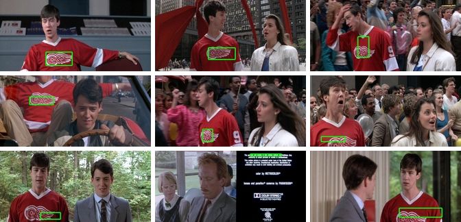
work, we first define the localized similarity between a We show the performance of ESS in localized retrieval
query region with bovw-histogram hQ and an image I as by applying it to 10143 keyframes of the full-feature movie
”Ferris Bueller’s Day Off”. Each frame is 880×416 pixels
locsim(I, Q) = max −χ2 (hQ , hR ) (6) large. For a given query, multi-image ESS is used to return
R⊆I
the 100 images containing the most similar regions. Fig-
where hR is the histogram for the subimage R and ure 6 shows a query region and some search results. Since
keyframes within the same scene tend to look very similar,
K we show only one image per scene. ESS is able to reliably
X (hQ − hR )2
χ2 (hQ , hR ) = k k
. (7) identify the Red Wings logo in different scenes regardless
k=1
hQk + hRk of strong background variations with only 4 falsely reported
frames out of 100. The first error occurred at position 88.
The retrieval task is now to identify the N images with high- The search required less than 2s per returned image, scal-
est localized similarity to Q as well as the region within ing linearly in the number of output images and effectively
each of them that best matches the query. sublinearly in the number of images in the database4 .
Since locsim consists of a maximization over all sub- 4 Since every image has to be inserted into the search queue, the method
regions in an image, we can use ESS to calculate it. To cannot be sublinear in the sense of computation complexity. However, the
construct the required bound, we first notice that the value observed growth of runtimes is sublinear, and the more images are added,
of each histogram bin over a set of rectangles R can be the fewer operations per image are necessary on average to find the top N .[4] T. M. Breuel. Fast Recognition using Adaptive Subdivisions
of Transformation Space. In CVPR, pages 445–451, 1992.
[5] O. Chapelle, P. Haffner, and V. N. Vapnik. Support Vector
Machines for Histogram-based Image Classification. Neural
Networks, 10(5):1055–1064, 1999.
(a) Red Wings logo used as query. (b) Top results of local search [6] O. Chum and A. Zisserman. An Exemplar Model for Learn-
ing Object Classes. In CVPR, 2007.
Figure 6. Image retrieval using a local χ2 distance: the Red Wings
[7] N. Dalal and B. Triggs. Histograms of Oriented Gradients
logo (left) is used as a query region. b) shows the top results (one
for Human Detection. In CVPR, pages 886–893, 2005.
image per scene). The center image in the bottom row contains a
[8] G. Dorko and C. Schmid. Selection of Scale-Invariant Parts
false positive. The other images are correct detections.
for Object Class Recognition. ICCV, pages 634–640,2003.
[9] M. Everingham, A. Zisserman, C. Williams, and L. V. Gool.
6. Conclusion The Pascal Visual Object Classes Challenge 2006 Results.
Technical report, PASCAL Network, 2006.
We have demonstrated how to perform fast object lo- [10] R. Fergus, P. Perona, and A. Zisserman. Object Class Recog-
calization and localized retrieval with results equivalent to nition by Unsupervised Scale-Invariant Learning. In CVPR,
an exhaustive evaluation of a quality function over all rect- pages 264–271, 2003.
angular regions in an image down to single pixel resolu- [11] V. Ferrari, L. Fevrier, F. Jurie, and C. Schmid. Groups of
Adjacent Contour Segments for Object Detection. PAMI,
tion. Sliding window approaches have the same goal, but in
30:36–51, 2008.
practice they have to resort to subsampling techniques and
[12] M. Fritz, B. Leibe, B. Caputo, and B. Schiele. Integrating
approximations to achieve a reasonable speed. In contrast Representative and Discriminative Models for Object Cate-
to this, our method retains global optimally in its search, gory Detection. In ICCV, pages 1363–1370, 2005.
which guarantees that no maxima of the quality function [13] D. Keysers, T. Deselaers, and T. M. Breuel. Optimal Ge-
are missed or misplaced. ometric Matching for Patch-Based Object Detection. EL-
The gain in speed and robustness allows the use of bet- CVIA, 6(1):44–54, 2007.
ter local classifiers (e.g. SVM with spatial pyramid kernel, [14] S. Lazebnik, C. Schmid, and J. Ponce. Beyond Bags of Fea-
nearest neighbor with χ2 -distance), for which we demon- tures: Spatial Pyramid Matching for Recognizing Natural
strated excellent results on the UIUC Cars, the PASCAL Scene Categories. In CVPR, pages 2169–2178,2006.
VOC 2006 dataset and in the VOC 2007 challenge. We also [15] B. Leibe, A. Leonardis, and B. Schiele. Robust Object De-
tection with Interleaved Categorization and Segmentation.
showed how to integrate additional properties, e.g. shape
IJCV Special Issue on Learning for Recognition and Recog-
penalties, and how to search over large image collections in nition for Learning, 2007 (in press).
sublinear time. [16] F.-F. Li and P. Perona. A Bayesian Hierarchical Model for
In future work, we plan to study the applicability of ESS Learning Natural Scene Categories. In CVPR, pages 524–
to further kernel-based classifiers. We are also working on 531, 2005.
extensions to other parametric shapes, like groups of boxes, [17] D. G. Lowe. Distinctive Image Features from Scale-Invariant
circles and ellipses. These are often more desirable in appli- Keypoints. IJCV, 60(2):91–110, 2004.
cations of biological, medical or industrial machine vision, [18] J. Mutch and D. G. Lowe. Multiclass Object Recognition
where high speed and performance guarantees are impor- with Sparse, Localized Features. In CVPR, pages 11–18,
tant quality factors as well. 2006.
[19] H. A. Rowley, S. Baluja, and T. Kanade. Human Face Detec-
tion in Visual Scenes. In NIPS 8, pages 875–881, 1996.
Acknowledgments [20] B. Schölkopf and A. Smola. Learning With Kernels. MIT
Press, 2002.
This work was funded in part by the EC project CLASS,
[21] J. Sivic, B. C. Russell, A. A. Efros, A. Zisserman, and W. T.
IST 027978. The second author is supported by a Marie
Freeman. Discovering Objects and their Localization in Im-
Curie fellowship under the EC project PerAct, EST 504321. ages. In ICCV, pages 370–377, 2005.
[22] J. Sivic and A. Zisserman. Video Google: A Text Retrieval
References Approach to Object Matching in Videos. In ICCV, pages
1470–1477, 2003.
[1] S. Agarwal, A. Awan, and D. Roth. Learning to Detect [23] V. Viitaniemi and J. Laaksonen. Techniques for Still Image
Objects in Images via a Sparse, Part-Based Representation. Scene Classification and Object Detection. In ICANN (2),
PAMI, 26(11):1475–1490, 2004. volume 4132, pages 35–44, 2006.
[2] H. Bay, T. Tuytelaars, and L. J. Van Gool. SURF: Speeded [24] J. Zhang, M. Marszalek, S. Lazebnik, and C. Schmid. Local
Up Robust Features. In ECCV, pages 404–417, 2006. Features and Kernels for Classification of Texture and Object
[3] A. Bosch, A. Zisserman, and X. Muñoz. Representing Shape Categories: A Comprehensive Study. IJCV, 73(2):213–238,
with a Spatial Pyramid Kernel. In CIVR. 2007.You can also read