Active Learning for Deep Object Detection
←
→
Page content transcription
If your browser does not render page correctly, please read the page content below
Active Learning for Deep Object Detection

                                                          Clemens-Alexander Brust1 , Christoph Käding1,2 and Joachim Denzler1,2
                                                                  1 Computer   Vision Group, Friedrich Schiller University Jena, Germany
                                                                                    2 Michael Stifel Center Jena, Germany

                                                                                      {f author, s author}@uni-jena.de

                                         Keywords:     Active Learning, Deep Learning, Object Detection, YOLO, Continuous Learning, Incremental Learning

                                         Abstract:     The great success that deep models have achieved in the past is mainly owed to large amounts of labeled
arXiv:1809.09875v1 [cs.CV] 26 Sep 2018

                                                       training data. However, the acquisition of labeled data for new tasks aside from existing benchmarks is both
                                                       challenging and costly. Active learning can make the process of labeling new data more efficient by selecting
                                                       unlabeled samples which, when labeled, are expected to improve the model the most. In this paper, we
                                                       combine a novel method of active learning for object detection with an incremental learning scheme (Käding
                                                       et al., 2016b) to enable continuous exploration of new unlabeled datasets. We propose a set of uncertainty-
                                                       based active learning metrics suitable for most object detectors. Furthermore, we present an approach to
                                                       leverage class imbalances during sample selection. All methods are evaluated systematically in a continuous
                                                       exploration context on the PASCAL VOC 2012 dataset (Everingham et al., 2010).

                                         1    Introduction                                              over time or the distribution underlying the problem
                                                                                                        changes itself. We simulate such an environment us-
                                             Labeled training data is highly valuable and the           ing splits of the PASCAL VOC 2012 (Everingham
                                         basic requirement of supervised learning. Active               et al., 2010) dataset. With our proposed framework,
                                         learning aims to expedite the process of acquiring new         a deep object detection system can be trained in an
                                         labeled data, ordering unlabeled samples by the ex-            incremental manner while the proposed aggregation
                                         pected value from annotating them. In this paper, we           schemes enable selection of valuable data for annota-
                                         propose novel active learning methods for object de-           tion. In consequence, a deep object detector can ex-
                                         tection. Our main contributions are (i) an incremen-           plore unknown data and adapt itself involving mini-
                                         tal learning scheme for deep object detectors with-            mal human supervision. This combination results in a
                                         out catastrophic forgetting based on (Käding et al.,          complete system enabling continuously changing sce-
                                         2016b), (ii) active learning metrics for detection de-         narios.
                                         rived from uncertainty estimates and (iii) an approach
                                         to leverage selection imbalances for active learning.          1.1     Related Work
                                             While active learning is widely studied in classi-
                                         fication tasks (Kovashka et al., 2016; Settles, 2009),         Object Detection using CNNs An important con-
                                         it has received much less attention in the domain of           tribution to object detection based on deep learning is
                                         deep object detection. In this work, we propose meth-          R-CNN (Girshick et al., 2014). It delivers a consid-
                                         ods that can be used with any object detector that pre-        erable improvement over previously published slid-
                                         dicts a class probability distribution per object pro-         ing window-based approaches. R-CNN employs se-
                                         posal. Scores from individual detections are aggre-            lective search (Uijlings et al., 2013), an unsupervised
                                         gated into a score for the whole image (see Fig. 1). All       method to generate region proposals. A pre-trained
                                         methods rely on the intuition that model uncertainty           CNN performs feature extraction. Linear SVMs (one
                                         and valuable samples are likely to co-occur (Settles,          per class) are used to score the extracted features and
                                         2009). Furthermore, we show how the balanced se-               a threshold is applied to filter the large number of
                                         lection of new samples can improve the resulting per-          proposed regions. Fast R-CNN (Girshick, 2015) and
                                         formance of an incrementally learned system.                   Faster R-CNN (Ren et al., 2015) offer further im-
                                             In continuous exploration application scenarios,           provements in speed and accuracy. Later on, R-CNN
                                         e.g., in camera streams, new data becomes available            is combined with feature pyramids to enable efficient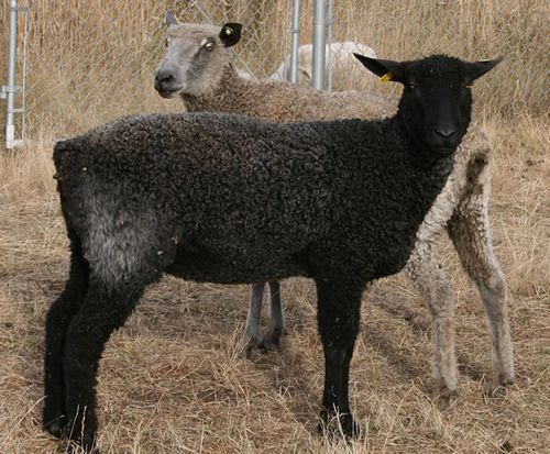
Score from
                                                                         margin sampling
                                                                            (1-vs-2)                +
                                                                                                                       Whole
                                                                                                                       image
                                                                                                                        score

                                                            ca

                                                            ca ycl
                                                            bir

                                                            hog
                                                            dot
                                                               c

                                                               rs
                                                                  e
                                                                    e
           Predict                                  Calculate scores                       Aggregate individual
      unlabeled example                            for each detection                            scores

Figure 1: Our proposed system for continuous exploration scenarios. Unlabeled images are evaluated by an deep object de-
tection method. The margins of predictions (i.e., absolute difference of highest and second-highest class score) are aggregated
to identify valuable instances by combining scores of individual detections.

multi-scale detections (Lin et al., 2017). YOLO (Red-              narasimhan and Grauman, 2014). A part-based de-
mon et al., 2016) is a more recent deep learning-based             tector for SVM classifiers in combination with hash-
object detector. Instead of using a CNN as a black box             ing is proposed for use in large-scale settings. Active
feature extractor, it is trained in an end-to-end fashion.         learning is realized by selecting the most uncertain in-
All detections are inferred in a single pass (hence the            stances for labeling. In (Roy et al., 2016), object de-
name “You Only Look Once”) while detection and                     tection is interpreted as a structured prediction prob-
classification are capable of independent operation.               lem using a version space approach in the so called
YOLOv2 (Redmon and Farhadi, 2017) and YOLOv3                       “difference of features” space. The authors propose
(Redmon and Farhadi, 2018) improve upon the orig-                  different margin sampling approaches estimating the
inal YOLO in several aspects. These include among                  future margin of an SVM classifier.
others different network architectures, different priors               Like our proposed approach, most related meth-
for bounding boxes and considering multiple scales                 ods presented above rely on uncertainty indicators
during training and detection. SSD (Liu et al., 2016)              like least confidence or 1-vs-2. However, they are
is a single-pass approach comparable to YOLO intro-                designed for a specific type of object detection and
ducing improvements like assumptions about the as-                 therefore can not be applied to deep object detection
pect ratio distribution of bounding boxes as well as               methods in general whereas our method can. Addi-
predictions on different scales. As a result of a series           tionally, our method does not propose single objects
of improvements, it is both faster and more accurate               to the human annotator. It presents whole images at
than the original YOLO. DSSD (Fu et al., 2017) fur-                once and requests labels for every object.
ther improves upon SSD in focusing more on context
with the help of deconvolutional layers.
                                                                   Active Learning for Deep Architectures In (Wang
                                                                   and Shang, 2014) and (Wang et al., 2016),
Active Learning for Object Detection The authors                   uncertainty-based active learning criteria for deep
of (Abramson and Freund, 2006) propose an active                   models are proposed. The authors offer several met-
learning system for pedestrian detection in videos                 rics to estimate model uncertainty, including least
taken by a camera mounted on the front of a mov-                   confidence, margin or entropy sampling. Wang et al.
ing car. Their detection method is based on AdaBoost               additionally describe a self-taught learning scheme,
while sampling of unlabeled instances is realized by               where the model’s prediction is used as a label for fur-
hand-tuned thresholding of detections. Object detec-               ther training if uncertainty is below a threshold. An-
tion using generalized Hough transform in combina-                 other type of margin sampling is presented in (Stark
tion with randomized decision trees, called Hough                  et al., 2015). The authors propose querying samples
forests, is presented in (Yao et al., 2012). Here,                 according to the quotient of the highest and second-
costs are estimated for annotations, and instances with            highest class probability. The visual detection of de-
highest costs are selected for labeling. This follows              fects using a ResNet is presented in (Feng et al.,
the intuition that those examples are most likely to               2017). The authors propose two methods: uncertainty
be difficult and therefore considered most valuable.               sampling (i.e., defect probability of 0.5) and positive
Another active learning approach for satellite images              sampling (i.e., selecting every positive sample since
using sliding windows in combination with an SVM                   they are very rare) for querying unlabeled instances
classifier and margin sampling is proposed in (Bietti,             as model update after labeling. Another work which
2012). The combination of active learning for object               presents uncertainty sampling is (Liu et al., 2017). In
detection with crowd sourcing is presented in (Vijaya-             addition, a query by committee strategy as well as ac-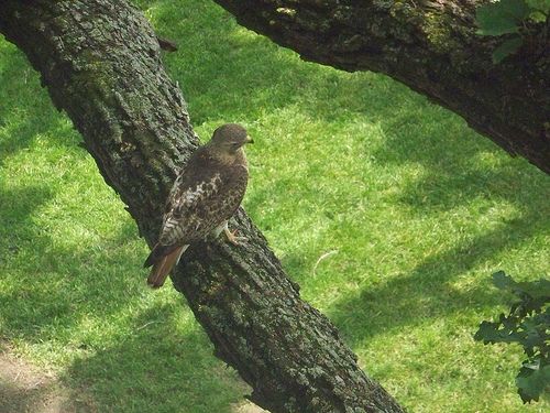
tive learning involving weighted incremental dictio-           For example, if the difference between the two
nary learning for active learning are proposed. In the     highest class scores is very low, the example may be
work of (Gal et al., 2017), several uncertainty-related    located close to a decision boundary. In this case, it
measures for active learning are presented. Since they     can be used to refine the decision boundary and is
use Bayesian CNNs, they can make use of the proba-         therefore valuable. The metric is defined using the
bilistic output and employ methods like variance sam-      highest scoring classes c1 and c2 :
pling, entropy sampling or maximizing mutual infor-                                                        2
mation. Finally, the authors of (Beluch et al., 2018)       v1vs2 (x) = 1 − (max p̂(c1 |x) − max p̂(c2 |x)) .
                                                                              c1 ∈K          c2 ∈K\c1
show that ensamble-based uncertainty measures are                                                               (1)
able to perform best in their evaluation. All of the           This procedure is known as 1-vs-2 or margin sam-
works introduced above are tailored to active learn-       pling (Settles, 2009). We use 1-vs-2 as part of our
ing in classification scenarios. Most of them rely on      methods since its operation is intuitive and it can pro-
model uncertainty, similar to our applied selection cri-   duce better estimates than e.g., least confidence ap-
teria.                                                     proaches (Käding et al., 2016a). However, our pro-
    Besides estimating the uncertainty of the model,       posed aggregation method could be applied to any
further retraining-based approaches are maximizing         other active learning measure.
the expected model change (Huang et al., 2016) or
the expected model output change (Käding et al.,
2016a) that unlabeled samples would cause after la-
beling. Since each bounding box inside an image has        3     Active Learning for Deep Object
to be evaluated according its active learning score,             Detection
both measures would be impractical in terms of run-
time without further modifications. A more complete            Using a classification metric on a single detec-
overview of general active learning strategies can be      tion is straightforward, if class scores are available.
found in (Kovashka et al., 2016; Settles, 2009).           Though, aggregating metrics of individual detections
                                                           for a complete image can be done in many different
                                                           ways. In the section below, we propose simple and
                                                           efficient aggregation strategies. Afterwards, we dis-
2    Prerequisite: Active Learning                         cuss the problem of class imbalance in datasets.

    In active learning, a value or metric v(x) is as-      3.1    Aggregation of Detection Metrics
signed to any unlabeled example x to determine its
possible contribution to model improvement. The            Possible aggregations include calculating the sum, the
current model’s output can be used to estimate a           average or the maximum over all detections. How-
value, as can statistical properties of the example it-    ever, for some aggregations, it is not clear how an im-
self. A high v(x) means that the example should be         age without any detections should be handled.
preferred during selection because of its estimated
value for the current model.
    In the following section, we propose a method to       Sum A straightforward method of aggregation is
adapt an active learning metric for classification to      the sum. Intuitively, this method prefers images with
object detection using an aggregation process. This        lots of uncertain detections in them. When aggregat-
method is applicable to any object detector whose out-     ing detections using a sum, empty examples should
put contains class scores for each detected object.        be valued zero. It is the neutral element of addition,
                                                           making it a reasonable value for an empty sum. A low
                                                           valuation effectively delays the selection of empty ex-
Classification For classification, the model output        amples until there are either no better examples left or
for a given example x is an estimated distribution of      the model has improved enough to actually produce
class scores p̂(c|x) over classes K. This distribution     detections on them. The value of a single example x
can be analyzed to determine whether the model made        can be calculated from the detections D in the follow-
an uncertain prediction, a good indicator of a valu-       ing way:
able example. Different measures of uncertainty are                      vSum (x) = ∑ v1vs2 (xi ) .             (2)
a common choice for selection, e.g., (Ertekin et al.,                                 i∈D
2007; Fu and Yang, 2015; Hoi et al., 2006; Jain and
Kapoor, 2009; Kapoor et al., 2010; Käding et al.,         Average Another possibility is averaging each de-
2016c; Tong and Koller, 2001; Beluch et al., 2018).        tection’s scores. The average is not sensitive to the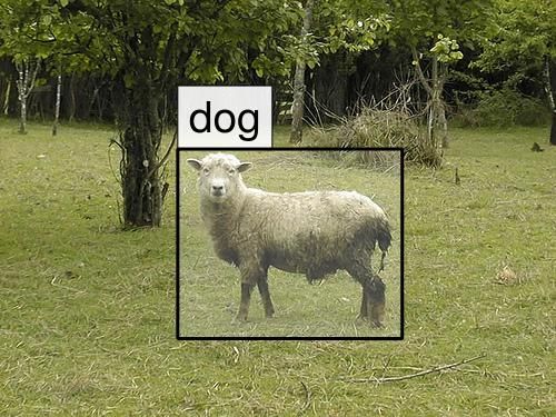
number of detections, which may make scores more            Data We use the PASCAL VOC 2012 dataset (Ev-
comparable between images. If a sample does not             eringham et al., 2010) to assess the effects of our
contain any detections, it will be assigned a zero          methods on learning. To specifically measure incre-
score. This is an arbitrary rule because there is no true   mental and active learning performance, both train-
neutral element w.r.t. averages. However, we choose         ing and validation set are split into parts A and B
zero to keep the behavior in line with the other met-       in two different random ways to obtain more gen-
rics:                                                       eral experimental results. Part B is considered “new”
                           1                                and is comprised of images with the object classes
             vAvg (x) =        ∑ v1vs2 (xi ) .        (3)
                          |D| i∈D                           bird, cow and sheep (first way) or tvmonitor, cat
                                                            and boat (second way). Part A contains all other 17
Maximum Finally, individual detection scores can            classes and is used for initial training. The training set
be aggregated by calculating the maximum. This can          for part B contains 605 and 638 images for the first
result in a substantial information loss. However, it       and second way, respectively. The decision towards
may also prove beneficial because of increased ro-          VOC in favor of recently published datasets was mo-
bustness to noise from many detections. For the max-        tivated by the conditions of the dataset itself. Since
imum aggregation, a zero score for empty examples           it mainly contains images showing fewer objects, it is
is valid. The maximum is not affected by zero valued        possible to split the data into a known and unknown
detections, because no single detection’s score can be      part without having images containing classes from
lower than zero:                                            both parts of the splits.

             vMax (x) = max v1vs2 (xi ) .            (4)
                           i∈D                              Active Exploration Protocol Before an experi-
                                                            mental run, the part B datasets are divided randomly
3.2    Handling Selection Imbalances                        into unlabeled batches of ten samples each. This fixed
                                                            assignment decreases the probability of very similar
Class imbalances can lead to worse results for classes      images being selected for the same batch compared
underrepresented in the training set. In a continu-         to always selecting the highest valued samples, which
ous learning scenario, this imbalance can be coun-          would lead to less diverse batches. This is valuable
tered during selection by preferring instances where        while dealing with data streams, e.g., from camera
the predicted class is underrepresented in the training     traps, or data with low intra-class variance. The con-
set. An instance is weighted by the following rule:         struction of diverse unlabeled data batches is a well
                    #instances + #classes                   known topic in batch-mode active learning (Settles,
             wc =                         ,          (5)    2009). However, the construction of diverse batches
                       #instancesc + 1
                                                            could lead to unintended side-effects and an evalua-
where c denotes the predicted class. We assume a            tion of those is beyond the scope of the current study.
symmetric Dirichlet prior with α = 1, meaning that          The unlabeled batch size is a trade-off between a tight
we have no prior knowledge of the class distribution,       feedback loop (smaller batches) and computational
and estimate the posterior after observing the total        efficiency (larger batches). As side-effect of the fixed
number of training instances as well as the number          batch assignment, there are some samples left over
of instances of class c in the training set. The weight     during selection (i.e., five for first way and eight for
wc is then defined as the inverse of the posterior to       second way of splitting).
prefer underrepresented classes. It is multiplied with          The unlabeled batches are assigned a value using
v1vs2 (x) before aggregation to obtain a final score.       the sum of the active learning metric over all images
                                                            in the corresponding batch as a meta-aggregation.
                                                            Other functions such as average or maximum could
4     Experiments                                           be considered too, but are also beyond the scope of
                                                            this paper.
    In the following, we present our evaluation. First          The highest valued batch is selected for an incre-
we show how the proposed aggregation metrics are            mental training step (Käding et al., 2016b). The net-
able to enhance recognition performance while se-           work is updated using the annotations from the dataset
lecting new data for annotation. After this, we will        in lieu of a human annotator. Please note, annotations
analyze the gained improvements when our proposed           are not needed for update batch selection but for the
weighting scheme is applied. This paper describes           update itself. This process is repeated from the point
work in progress. Code will be made available after         of batch valuation until there are no unlabeled batches
conference publication.                                     left. The assignment of samples to unlabeled batches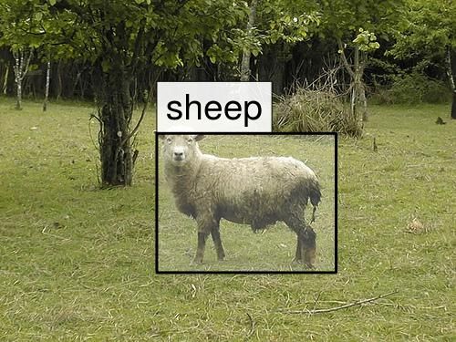
is not changed during an experimental run.                 are added. Because of the design of YOLO’s out-
                                                           put layer, we rearrange the weights to fit new classes,
                                                           adding 49 weights per class.
Evaluation We report mean average precision
(mAP) as described in (Everingham et al., 2010) and
validate each five new batches (i.e., 50 new samples).
                                                           4.1    Results
The result is averaged over five runs for each active
learning metric and way of splitting for a total of ten    We focus our analysis on the new, unknown data.
runs. As a baseline for comparison, we evaluate the        However, not losing performance on known data is
performance of random selection, since there is no         also important. We analyze the performance on the
other work suitable for direct comparison without any      known part of the data (i.e., part A of the VOC
adjustments as of yet.                                     dataset) to validate our method. In worst case, the
                                                           mAP decreases from 36.7% initially to 32.1% aver-
                                                           aged across all experimental runs and methods al-
Setup – Object Detector We use YOLO as deep                though three new classes were introduced. We can see
object detection framework (Redmon et al., 2016).          that the incremental learning method from (Käding
More precisely, we use the YOLO-Small architecture         et al., 2016b) causes only minimal losses on known
as an alternative to larger object detection networks,     data. These losses in performance are also referred to
because it allows for much faster training. Our ini-       as “catastrophic forgetting” in literature (Kirkpatrick
tial model is obtained by fine-tuning the Extraction       et al., 2016). The method from (Käding et al., 2016b)
model1 on part A of the VOC dataset for 24,000 it-         does not require additional model parameters or ad-
erations using the Adam optimizer (Kingma and Ba,          justed loss terms for added samples like comparable
2014), for each way of splitting the dataset into parts    approaches such as (Shmelkov et al., 2017) do, which
A and B, resulting in two initial models. The first half   is important for learning indefinitely.
of initial training is completed with a learning rate of        Performance of active learning methods is usu-
0.0001. The second half and all incremental experi-        ally evaluated by observing points on a learning curve
ments use a lower learning rate of 0.00001 to prevent      (i.e., performance over number of added samples). In
divergence. Other hyperparameters match (Redmon            Table 1, we show the mAP for the new classes from
et al., 2016), including the augmentation of training      part B of VOC at several intermediate learning steps
data using random crops, exposure or saturation ad-        as well as exhausting the unlabeled pool. In addition
justments.                                                 we show the area under learning curve (AULC) to fur-
                                                           ther improve comparability among the methods. In
                                                           our experiments, the number of samples added equals
Setup – Incremental Learning Extending an exist-           the number of images.
ing CNN without sacrificing performance on known
data is not a trivial task. Fine-tuning exclusively on
new data leads to a severe degradation of performance      Quantitative Results – Fast Exploration Gaining
on previously learned examples (Kirkpatrick et al.,        accuracy as fast as possible while minimizing the hu-
2016; Shmelkov et al., 2017). We use a straightfor-        man supervision is one of the main goals of active
ward, but effective fine-tuning method (Käding et al.,    learning. Moreover, in continuous exploration sce-
2016b) to implement incremental learning. With each        narios, like faced in camera feeds or other continuous
gradient step, the mini-batch is constructed by ran-       automatic measurements, it is assumed that new data
domly selecting from old and new examples with a           is always available. Hence, the pool of valuable ex-
certain probability of λ or 1 − λ, respectively. After     amples will rarely be exhausted. To assess the perfor-
completing the learning step, the new data is simply       mance of our methods in this fast exploration context,
considered old data for the next step. This method         we evaluate the models after learning learning small
can balance known and unknown data performance             amounts of samples. At this point there is still a large
successfully. We use a value of 0.5 for λ to make as       number of diverse samples for the methods to choose
few assumptions as possible and perform 100 itera-         from, which makes the following results much more
tions per update. Algorithm 1 describes the protocol       relevant for practical applications than results on the
in more detail. The method can be applied to YOLO          full dataset.
object detection with some adjustments. Mainly, the            In general, we can see that incremental learning
architecture needs to be changed when new classes          works in the context of the new classes in part B of the
                                                           data, meaning that we observe an improving perfor-
   1 http://pjreddie.com/media/files/                      mance for all methods. After adding only 50 samples,
extraction.weights                                         Max and Avg are performing better than passive selec-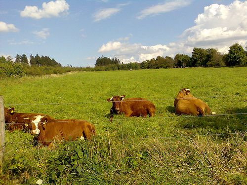
Algorithm 1: Detailed description of the experimental protocol. Please note that in an actual continuous learning scenario,
new examples are always added to U. The loop is never left because U is never exhausted. The described splitting process
would have to be applied regularly.
Require: Known labeled samples L, unknown samples U, initial model f0 , active learning metric v

  U = U1 , U2 , . . . ← split of U into random batches
  f ← f0

  while U is not empty do
     calculate scores for all batches in U using f
     Ubest ← highest scoring batch in U according to v

      Ybest ← annotations for Ubest human-machine interaction
      f ← incrementally train f using L and (Ubest , Ybest )

     U ← U\Ubest
     L ← L ∪ (Ubest , Ybest )
  end while
Table 1: Validation results on part B of the VOC data (i.e., new classes only). Bold face indicates block-wise best results, i.e.,
best results with and without additional weighting (· + w). Underlined face highlights overall best results.
                   50 samples        100 samples        150 samples        200 samples       250 samples        All samples
                   mAP/AULC          mAP/AULC           mAP/AULC           mAP/AULC          mAP/AULC           mAP/AULC
  Baseline
   Random            8.7 / 4.3        12.4 / 14.9        15.5 / 28.8       18.7 / 45.9        21.9 / 66.2        32.4 / 264.0
  Our Methods
   Max               9.2 / 4.6        12.9 / 15.7        15.7 / 30.0       19.8 / 47.8        22.6 / 69.0        32.0 / 269.3
   Avg               9.0 / 4.5        12.4 / 15.2        15.8 / 29.2       19.3 / 46.8        22.7 / 67.8        33.3 / 266.4
   Sum               8.5 / 4.2        14.3 / 15.6        17.3 / 31.4       19.8 / 49.9        22.7 / 71.2        32.4 / 268.2
   Max + w           9.2 / 4.6        13.0 / 15.7        17.0 / 30.7       20.6 / 49.5        23.2 / 71.4        33.0 / 271.0
   Avg + w           8.7 / 4.3        12.5 / 14.9        16.6 / 29.4       19.9 / 47.7        22.4 / 68.8        32.7 / 267.1
   Sum + w           8.7 / 4.4        13.7 / 15.6        17.5 / 31.2       20.9 / 50.4        24.3 / 72.9        32.7 / 273.6

tion while the Sum metric is outperformed marginally.               stages, it helps to gain noticeable improvements. Es-
When more and more samples are added (i.e., 100 to                  pecially for the Sum method benefits from the sam-
250 samples), we observe a superior performance of                  ple weighting scheme. A possible explanation for this
the Sum aggregation. But also the two other aggre-                  behavior would be the following: At early stages, the
gation techniques are able to reach better rates than               classifier has not seen many samples of each class and
mere random selection. We attribute the fast increase               therefore suffers more from miss-classification errors.
of performance for the Sum metric to its tendency to                Hence, the weighting scheme is not able to encourage
select samples with many object inside which leads to               the selection of rare class samples since the classi-
more annotated bounding boxes. However, the target                  fier decisions are still too unstable. At later stages,
application is a scenario where the amount of unla-                 this problem becomes less severe and the weighting
beled data is huge or new data is approaching contin-               scheme is much more helpful than in the beginning.
uously and hence a complete evaluation by humans is                 This could also explain the performance of Sum in
infeasible. Here, we consider the amount of images to               general. Further details on learning pace are given
be evaluated more critical as the time needed to draw               later in a qualitative study on model evolution. Addi-
single bounding boxes. Another interesting fact is the              tionally, the Sum aggregation tends to select batches
almost equal performance of Max and Avg which can                   with many detections in it. Hence, it is natural that
be explained as follows: the VOC dataset consists                   the improvement is noticeable the most with this ag-
mostly of images with only one object in them. There-               gregation technique since it helps to find batches with
fore, both metrics lead to a similar score if objects are           many rare objects in it.
identified correctly.
    We can also see that the proposed balance han-
dling (i.e., · + w) causes slight losses in performance             Quantitative Results – All Available Samples In
at very early stages up to 100 samples. At subsequent               our case, active learning only affects the sequence of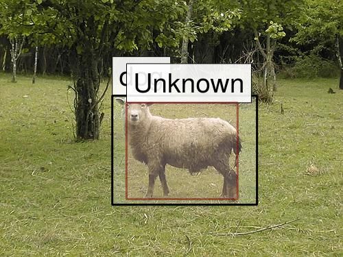
unlabeled batches if we train until there is no new data
available. Therefore, there are only very small differ-
ences between each method’s results for mAP after
training has completed. The small differences indi- bird cow
cate that the chosen incremental learning technique 30
(Käding et al., 2016b) is suitable for the faced sce- 30
nario. In continuous exploration, it is usually assumed 20
AP (%)
AP (%)
that there will be more new unlabeled data available 20
than can be processed. Nevertheless, evaluating the
10
long term performance of our metrics is important to 10 Sum Sum
detect possible deterioration over time compared to Sum + w Sum + w
random selection. In contrast to this, the differences 0 0
in AULC arise from the improvements of the different 0 250 500 0 250 500
# samples # samples
methods during the experimental run and therefore
should be considered as distinctive feature implying sheep boat
the performance over the whole experiment. Having
this in mind, we can still see that Sum performs best 20 20
while the weighting generally leads to improvements.
AP (%)
AP (%)
10 10
Quantitative Results — Class-wise Analysis To
validate the efficacy of our sample weighting strategy Sum Sum
Sum + w Sum + w
as discussed in Section 3.2, it is important to measure 0 0
not only overall performance, but to look at metrics 0 250 500 0 250 500
for individual classes. Fig. 2 shows the performance # samples # samples
over time on the validation set for each individual
cat tvmonitor
class. For reference, we also provide the class distri- 60
bution over the relevant part of the VOC dataset, indi-
20
cated by number of object instances in total as well as
40
number of images with at least one instance in it.
AP (%)
AP (%)
In the first row, we observe an advantage for the 10
weighted method when looking at the performance of 20
Sum Sum
cow. Out of the three classes in this way of splitting
Sum + w Sum + w
cow has the fewest instances in the dataset. The per- 0 0
formance of tvmonitor in the second row shows a 0 250 500 0 250 500
similar pattern, where it is also the class with the low- # samples # samples
est number of object instances in the dataset. Ana-
lyzing bird and cat, the top classes by number of Number of samples in VOC dataset by class
instances in each way of splitting, we observe only
small differences in performance. Thus, we can show Objects
1000
evidence that our balancing scheme is able to improve Images
# samples
performance on rare classes while it does not effect
performance on frequent classes. 500
Intuitively, these observations are in line with our
expectations regarding our handling of class imbal- 0
ances, where examples of rare classes should be pre- bird cow sheep boat cat tvmonitor
ferred during selection. We start to observe the advan-
Figure 2: Class-wise validation results on part B of the VOC
tages after around 100 training examples, because, for dataset (i.e.,, unknown classes). The first row details the
the selection to happen correctly, the prediction of the first way of splitting (bird,cow,sheep) while the second
rare class needs to be correct in the first place. row shows the second way (boat,cat,tvmonitor). For ref-
erence, the distribution of samples (object instances as well
as images with at least one instance) over the VOC dataset
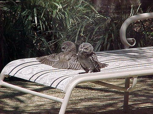
Qualitative Results – Sample Valuation We cal- is provided in the third row.
culate whole image scores over bird, cow and sheep
samples using our corresponding initial model trained
on the remaining classes for the first way of splitting.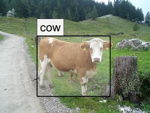
Most valuable examples (highest score)

 Sum (+ w)

Avg (+ w)

Max (+ w)

                                          Least valuable examples (zero score)

 All

Figure 3: Value of examples of cow, sheep and bird as determined by the Sum, Avg and Max metrics using the initial model.
The top seven selection is not affected by using our weighting method to counter training set class imbalaces.

Figure 3 shows those images that the three aggrega-            as visually similar dog, horse and cat. bird is often
tion metrics consider the most valuable. Additionally,         classified as aeroplane. After selecting and learning
common zero scoring images are shown. The least                150 samples, the objects are detected and classified
valuable images shown here are representative of all           correctly and reliably.
proposed metrics because they do not lead to any de-               During the learning process, there are also un-
tections using the initial model. Note that there are          known objects. Please note, being able to mark ob-
more than seven images with zero score in the train-           jects as unknown is a direct consequence of using
ing dataset. The images shown in the figure have been          YOLO. Those objects have a detection confidence
selected randomly.                                             above the required threshold, but no classification is
    Intuitively, the Sum metric should prefer images           certain enough. This property of YOLO is important
with many objects in them over single objects, even if         for the discovery of objects of new classes. Never-
individual detection values are low. Although VOC              theless, if similar information is available from other
contains mostly of images with a single object, all            detection methods, our techniques could easily be ap-
seven of the highest scoring images contain at least           plied.
three objects. The Average and Maximum metric
prefer almost identical images since the average and
maximum are used to be nearly equal for few detec-
tions. With few exceptions, the most valuable images           5    Conclusions
contain pristine examples of each object. They are
well lit and isolated. The objects in the zero scoring             In this paper, we propose several uncertainty-
images are more noisy and hard to identify even for            based active learning metrics for object detection.
the human viewer, resulting in fewer reliable detec-           They only require a distribution of classification
tions.                                                         scores per detection. Depending on the specific task,
                                                               an object detector that will report objects of un-
                                                               known classes is also important. Additionally, we
Qualitative Results – Model Evolution Observing                propose a sample weighting scheme to balance selec-
the change in model output as new data is learned can          tions among classes.
help estimate the number of samples needed to learn                We evaluate the proposed metrics on the PASCAL
new classes and identify possible confusions. Fig. 4           VOC 2012 dataset (Everingham et al., 2010) and of-
shows the evolution from initial guesses to correct de-        fer quantitative and qualitative results and analysis.
tections after learning 150 samples, corresponding to          We show that the proposed metrics are able to guide
an fast exploration scenario. For selection, the Sum           the annotation process efficiently which leads to su-
metric is used.                                                perior performance in comparison to a random selec-
    The class confusions shown in the figure are typ-          tion baseline. In our experimental evaluation, the Sum
ical for this scenario. cow and sheep are recognized           metric is able to achieve best results overall which can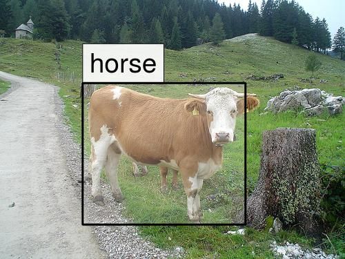
New classes (part B)                   Known classes (part A)
                                        bird           cow              sheep       aeroplane            car

                  Initial prediction

                  After 50 samples

                 After 150 samples

                               Figure 4: Evolution of detections on examples from validation set.

be attributed to the fact that it tends to select batches                   bles for active learning in image classification.
with many single objects in it. However, the targeted                       In Computer Vision and Pattern Recognition
scenario is an application with huge amounts of unla-                       (CVPR).
beled data where we consider the amount of images                      Bietti, A. (2012). Active learning for object detection
to be evaluated as more critical than the time needed                       on satellite images. Technical report, California
to draw single bounding boxes. Examples would be                            Institute of Technology, Pasadena.
camera streams or camera trap data. To expedite
annotation, our approach could be combined with a                      Ertekin, S., Huang, J., Bottou, L., and Giles, L.
weakly supervised learning approach as presented in                         (2007). Learning on the border: active learning
(Papadopoulos et al., 2016). We also showed that our                        in imbalanced data classification. In Conference
weighting scheme leads to even increased accuracies.                        on Information and Knowledge Management.
     All presented metrics could be applied to other                   Everingham, M., Van Gool, L., Williams, C. K. I.,
deep object detectors, such as the variants of SSD                          Winn, J., and Zisserman, A. (2010). The pascal
(Liu et al., 2016), the improved R-CNNs e.g., (Ren                          visual object classes (voc) challenge. Interna-
et al., 2015) or the newer versions of YOLO (Red-                           tional Journal of Computer Vision (IJCV).
mon and Farhadi, 2017). Moreover, our proposed                         Feng, C., Liu, M.-Y., Kao, C.-C., and Lee, T.-Y.
metrics are not restricted to deep object detection and                     (2017). Deep active learning for civil infrastruc-
could be applied to arbitrary object detection methods                      ture defect detection and classification. In Inter-
if they fulfill the requirements. It only requires a com-                   national Workshop on Computing in Civil Engi-
plete distribution of classifications scores per detec-                     neering (IWCCE).
tion. Also the underlying uncertainty measure could                    Fu, C.-J. and Yang, Y.-P. (2015). A batch-mode active
be replaced with arbitrary active learning metrics to                       learning svm method based on semi-supervised
be aggregated afterwards. Depending on the specific                         clustering. Intelligent Data Analysis.
task, an object detector that will report objects of un-
known classes is also important.                                       Fu, C.-Y., Liu, W., Ranga, A., Tyagi, A., and Berg,
     The proposed aggregation strategies also general-                      A. C. (2017). Dssd: Deconvolutional single shot
ize to selection of images based on segmentation re-                        detector. arXiv preprint arXiv:1701.06659.
sults or any other type of image partition. The result-                Gal, Y., Islam, R., and Ghahramani, Z. (2017). Deep
ing scores could also be applied in a novelty detection                     bayesian active learning with image data. arXiv
scenario.                                                                   preprint arXiv:1703.02910.
                                                                       Girshick, R. (2015). Fast R-CNN. In International
                                                                            Conference on Computer Vision (ICCV).
REFERENCES                                                             Girshick, R., Donahue, J., Darrell, T., and Malik,
                                                                            J. (2014). Rich feature hierarchies for accu-
Abramson, Y. and Freund, Y. (2006). Active learn-                           rate object detection and semantic segmenta-
    ing for visual object detection. Technical report,                      tion. In Computer Vision and Pattern Recogni-
    University of California, San Diego.                                    tion (CVPR).
Beluch, W. H., Genewein, T., Nürnberger, A., and                      Hoi, S. C., Jin, R., and Lyu, M. R. (2006). Large-scale
    Köhler, J. M. (2018). The power of ensem-                              text categorization by batch mode active learn-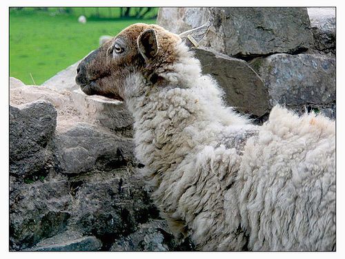
ing. In International Conference on World Wide         Papadopoulos, D. P., Uijlings, J. R. R., Keller, F., and
     Web (WWW).                                                  Ferrari, V. (2016). We dont need no bounding-
Huang, J., Child, R., Rao, V., Liu, H., Satheesh,                boxes: Training object class detectors using only
     S., and Coates, A. (2016). Active learning                  human verification. In Computer Vision and Pat-
     for speech recognition: the power of gradients.             tern Recognition (CVPR).
     arXiv preprint arXiv:1612.03226.                       Redmon, J., Divvala, S., Girshick, R., and Farhadi, A.
Jain, P. and Kapoor, A. (2009). Active learning for              (2016). You only look once: Unified, real-time
     large multi-class problems. In Computer Vision              object detection. In Computer Vision and Pattern
     and Pattern Recognition (CVPR).                             Recognition (CVPR).
Käding, C., Freytag, A., Rodner, E., Perino, A., and       Redmon, J. and Farhadi, A. (2017). Yolo9000: Better,
     Denzler, J. (2016a). Large-scale active learn-              faster, stronger. In Computer Vision and Pattern
     ing with approximated expected model output                 Recognition (CVPR).
     changes. In German Conference on Pattern               Redmon, J. and Farhadi, A. (2018).             Yolov3:
     Recognition (GCPR).                                         An incremental improvement. arXiv preprint
Käding, C., Rodner, E., Freytag, A., and Denzler, J.            arXiv:1804.02767.
     (2016b). Fine-tuning deep neural networks in           Ren, S., He, K., Girshick, R., and Sun, J. (2015).
     continuous learning scenarios. In ACCV Work-                Faster R-CNN: Towards real-time object detec-
     shop on Interpretation and Visualization of Deep            tion with region proposal networks. In Neural
     Neural Nets (ACCV-WS).                                      Information Processing Systems (NIPS).
Käding, C., Rodner, E., Freytag, A., and Denzler, J.       Roy, S., Namboodiri, V. P., and Biswas, A. (2016).
     (2016c). Watch, ask, learn, and improve: A life-            Active learning with version spaces for object
     long learning cycle for visual recognition. In              detection. arXiv preprint arXiv:1611.07285.
     European Symposium on Artificial Neural Net-
                                                            Settles, B. (2009). Active learning literature sur-
     works (ESANN).
                                                                 vey. Technical report, University of Wisconsin–
Kapoor, A., Grauman, K., Urtasun, R., and Darrell,               Madison.
     T. (2010). Gaussian processes for object cate-
     gorization. International Journal of Computer          Shmelkov, K., Schmid, C., and Alahari, K. (2017).
     Vision (IJCV).                                              Incremental learning of object detectors without
                                                                 catastrophic forgetting. In International Confer-
Kingma, D. P. and Ba, J. (2014). Adam: A method for
                                                                 ence on Computer Vision (ICCV).
     stochastic optimization. arXiv preprint arXiv:
     1412.6980.                                             Stark, F., Hazırbas, C., Triebel, R., and Cremers, D.
                                                                 (2015). Captcha recognition with active deep
Kirkpatrick, J., Pascanu, R., Rabinowitz, N. C., Ve-
                                                                 learning. In Workshop New Challenges in Neural
     ness, J., Desjardins, G., Rusu, A. A., Milan, K.,
                                                                 Computation.
     Quan, J., Ramalho, T., Grabska-Barwinska, A.,
     Hassabis, D., Clopath, C., Kumaran, D., and            Tong, S. and Koller, D. (2001). Support vector ma-
     Hadsell, R. (2016). Overcoming catastrophic                 chine active learning with applications to text
     forgetting in neural networks. arXiv preprint               classification. Journal of Machine Learning Re-
     arXiv:1612.00796.                                           search (JMLR).
Kovashka, A., Russakovsky, O., Fei-Fei, L., and             Uijlings, J. R., Van De Sande, K. E., Gevers, T.,
     Grauman, K. (2016). Crowdsourcing in com-                   and Smeulders, A. W. (2013). Selective search
     puter vision. Foundations and Trends in Com-                for object recognition. International Journal of
     puter Graphics and Vision.                                  Computer Vision (IJCV), 104(2):154–171.
Lin, T.-Y., Dollár, P., Girshick, R., He, K., Hariharan,   Vijayanarasimhan, S. and Grauman, K. (2014).
     B., and Belongie, S. (2017). Feature pyramid                Large-scale live active learning: Training object
     networks for object detection. In CVPR.                     detectors with crawled data and crowds. Inter-
Liu, P., Zhang, H., and Eom, K. B. (2017). Active                national Journal of Computer Vision (IJCV).
     deep learning for classification of hyperspectral      Wang, D. and Shang, Y. (2014). A new active labeling
     images. Selected Topics in Applied Earth Obser-             method for deep learning. In International Joint
     vations and Remote Sensing.                                 Conference on Neural Networks (IJCNN).
Liu, W., Anguelov, D., Erhan, D., Szegedy, C., Reed,        Wang, K., Zhang, D., Li, Y., Zhang, R., and Lin, L.
     S., Fu, C.-Y., and Berg, A. C. (2016). SSD: Sin-            (2016). Cost-effective active learning for deep
     gle shot multibox detector. In European Confer-             image classification. Circuits and Systems for
     ence on Computer Vision (ECCV).                             Video Technology.
Yao, A., Gall, J., Leistner, C., and Van Gool, L.
(2012). Interactive object detection. In Com-
puter Vision and Pattern Recognition (CVPR).You can also read