Multimodal Generative Learning Utilizing Jensen-Shannon-Divergence
←
→
Page content transcription
If your browser does not render page correctly, please read the page content below
Multimodal Generative Learning Utilizing
                                                         Jensen-Shannon-Divergence

                                                        Thomas M. Sutter                                Imant Daunhawer
                                                  Department of Computer Science                  Department of Computer Science
                                                           ETH Zurich                                      ETH Zurich
                                                  thomas.sutter@inf.ethz.ch                      imant.daunhawer@inf.ethz.ch
arXiv:2006.08242v2 [cs.LG] 5 Oct 2020

                                                                                  Julia E. Vogt
                                                                          Department of Computer Science
                                                                                   ETH Zurich
                                                                           julia.vogt@inf.ethz.ch

                                                                                      Abstract

                                                 Learning from different data types is a long-standing goal in machine learning
                                                 research, as multiple information sources co-occur when describing natural phe-
                                                 nomena. However, existing generative models that approximate a multimodal
                                                 ELBO rely on difficult or inefficient training schemes to learn a joint distribution
                                                 and the dependencies between modalities. In this work, we propose a novel, effi-
                                                 cient objective function that utilizes the Jensen-Shannon divergence for multiple
                                                 distributions. It simultaneously approximates the unimodal and joint multimodal
                                                 posteriors directly via a dynamic prior. In addition, we theoretically prove that
                                                 the new multimodal JS-divergence (mmJSD) objective optimizes an ELBO. In
                                                 extensive experiments, we demonstrate the advantage of the proposed mmJSD
                                                 model compared to previous work in unsupervised, generative learning tasks.

                                        1   Introduction
                                        Replicating the human ability to process and relate information coming from different sources and
                                        learn from these is a long-standing goal in machine learning [2]. Multiple information sources offer
                                        the potential of learning better and more generalizable representations, but pose challenges at the
                                        same time: models have to be aware of complex intra- and inter-modal relationships, and be robust
                                        to missing modalities [19, 31]. However, the excessive labelling of multiple data types is expensive
                                        and hinders possible applications of fully-supervised approaches [5, 11]. Simultaneous observations
                                        of multiple modalities moreover provide self-supervision in the form of shared information which
                                        connects the different modalities. Self-supervised, generative models are a promising approach to
                                        capture this joint distribution and flexibly support missing modalities with no additional labelling cost
                                        attached. Based on the shortcomings of previous work (see section 2.1), we formulate the following
                                        wish-list for multimodal, generative models:
                                        Scalability. The model should be able to efficiently handle any number of modalities. Translation
                                        approaches [10, 32] have had great success in combining two modalities and translating from one
                                        to the other. However, the training of these models is computationally expensive for more than two
                                        modalities due to the exponentially growing number of possible paths between subsets of modalities.
                                        Missing data. A multimodal method should be robust to missing data and handle any combination
                                        of available and missing data types. For discriminative tasks, the loss in performance should
                                        be minimized. For generation, the estimation of missing data types should be conditioned on

                                        Preprint. Under review.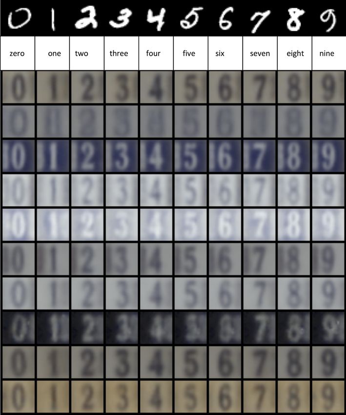
and coherent with available data while providing diversity over modality-specific attributes in the
generated samples.
Information gain. Multimodal models should benefit from multiple modalities for discriminative as
well as for generative tasks.
In this work, we introduce a novel probabilistic, generative and self-supervised multi-modal model.
The proposed model is able to integrate information from different modalities, reduce uncertainty and
ambiguity in redundant sources, as well as handle missing modalities while making no assumptions
about the nature of the data, especially about the inter-modality relations.
We base our approach directly in the Variational Bayesian Inference framework and propose the new
multimodal Jensen-Shannon divergence (mmJSD) objective. We introduce the idea of a dynamic prior
for multimodal data, which enables the use of the Jensen-Shannon divergence for M distributions [1,
16] and interlinks the unimodal probabilistic representations of the M observation types. Additionally,
we are - to the best of our knowledge - the first to empirically show the advantage of modality-specific
subspaces for multiple data types in a self-supervised and scalable setting. For the experiments, we
concentrate on Variational Autoencoders [13]. In this setting, our multimodal extension to variational
inference implements a scalable method, capable of handling missing observations, generating
coherent samples and learning meaningful representations. We empirically show this on two different
datasets. In the context of scalable generative models, we are the first to perform experiments on
datasets with more than 2 modalities showing the ability of the proposed method to perform well in a
setting with multiple modalities.

2     Theoretical Background & Related Work

We consider some dataset of N i.i.d. sets {X (i) }N i=1 with every X
                                                                      (i)
                                                                           being a set of M modalities
   (i)     (i) M
X = {xj }j=1 . We assume that the data is generated by some random process involving a joint
hidden random variable z where inter-modality dependencies are unknown. In general, the same
assumptions are valid as in the unimodal setting [13]. The marginal log-likelihood can be decomposed
                                                                                    PN
into a sum over marginal log-likelihoods of individual sets log pθ ({X (i) }N
                                                                            i=1 ) =
                                                                                                    (i)
                                                                                       i=1 log pθ (X ),
which can be written as:
                   log pθ (X (i) ) =KL(qφ (z|X (i) )||pθ (z|X (i) )) + L(θ, φ; X (i) ),              (1)

            with L(θ, φ; X (i) ) :=Eqφ (z|X) [log pθ (X (i) |z)] − KL(qφ (z|X (i) )||pθ (z)).        (2)
L(θ, φ; X (i) ) is called evidence lower bound (ELBO) on the marginal log-likelihood of set i.
The ELBO forms a computationally tractable objective to approximate the joint data distribution
log pθ (X (i) ) which can be efficiently optimized, because it follows from the non-negativity of the
KL divergence: log pθ (X (i) ) ≥ L(θ, φ; X (i) ). Particular to the multimodal case is what happens to
the ELBO formulation if one or more data types are missing: we are only able to approximate the
                                                                     (i)     (i)
true posterior pθ (z|X (i) ) by the variational function qφK (z|XK ). XK denotes a subset of X (i)
with K available modalities where K ≤ M . However, we would still like to be able to approximate
the true multimodal posterior distribution pθ (z|X (i) ) of all data types. For simplicity, we always use
   (i)
XK to symbolize missing data for set i, although there is no information about which or how many
modalities are missing. Additionally, different modalities might be missing for different sets i. In this
case, the ELBO formulation changes accordingly:
                                                                                   (i)
          LK (θ, φK ; X (i) ) :=Eq        (i)   [log(pθ (X (i) |z)] − KL(qφK (z|XK )||pθ (z))        (3)
                                   φK (z|XK )

                                                     (i)
LK (θ, φK ; X (i) ) defines the ELBO if only XK is available, but we are interested in the true
posterior distribution pθ (z|X (i) ). To improve readability, we will omit the superscript (i) in the
remaining part of this work.

2.1   Related Work

In this work, we focus on methods with the aim of modelling a joint latent distribution, instead of
transferring between modalities [10, 26] due to the scalability constraint described in section 1.

                                                     2
Joint and Conditional Generation. [25] implemented a multimodal VAE and introduced the idea
that the distribution of the unimodal approximation should be close to the multimodal approximation
function. [29] introduced the triple ELBO as an additional improvement. Both define labels as second
modality and are not scalable in number of modalities.
Modality-specific Latent Subspaces. [9] and [28] both proposed models with modality-specific
latent distributions and an additional shared distribution. The former relies on supervision by labels
to extract modality-independent factors, while the latter is non-scalable.
Scalability. More recently, [14] and [30] proposed scalable multimodal generative models for which
they achieve scalability by using a Product of Experts [8] as a joint approximation distribution.
The Product of Experts (PoE) allows them to handle missing modalities without requiring separate
inference networks for every combination of missing and available data. A PoE is computationally
attractive as - for Gaussian distributed experts - it remains Gaussian distributed which allows the
calculation of the KL-divergence in closed form. However, they report problems in optimizing
the unimodal variational approximation distributions due to the multiplicative nature of the PoE.
To overcome this limitation, [30] introduced a combination of ELBOs which results in the final
objective not being an ELBO anymore. [24] use a Mixture-of-Experts (MoE) as joint approximation
function. The additive nature of the MoE facilitates the optimization of the individual experts, but is
computationally less efficient as there exists no closed form solution to calculate the KL-divergence.
[24] need to rely on importance sampling (IS) to achieve the desired performance. IS based VAEs [4]
tend to achieve tight ELBOs for the price of a reduced computational efficiency. Additionally, their
model leverages M 2 passes through the decoder networks which increases the computational cost
further.

3     The multimodal JS-Divergence model
We propose a new multimodal objective (mmJSD) utilizing the Jensen-Shannon divergence. Com-
pared to previous work, this formulation does not need any additional training objectives [30],
supervision [28] or importance sampling [24], while being scalable [9].
Definition 1. We define a new objective L(θ,
                                          e φ; X) for learning multimodal, generative models
which utilizes the Jensen-Shannon divergence:
             e φ; X) := Eq (z|X) [log pθ (X|z)] − JS M +1 ({qφ (z|xj )}M , pθ (z))
            L(θ,                                                                            (4)
                              φ                             π          zj         j=1

where JSπM +1 denotes the Jensen-Shannon
                                     P        divergence for M + 1 distributions with distribution
weights π = [π1 , . . . , πM +1 ] and πi = 1.
For any P ∈ N, P ≥ 2, the Jensen-Shannon (JS) divergence for P distributions is defined as follows:
                                             P
                                             X
                     JSπP ({qj (z)}P
                                   j=1 ) =         πj KL(qj (z)|fM ({qν (z)}P
                                                                            ν=1 )                  (5)
                                             j=1

where the function fM defines a mixture distribution of its arguments. The JS-divergence for P
distributions is the extension of the standard JS-divergence for two distributions to an arbitrary
number of distributions. It is a weighted sum of KL-divergences between the P individual probability
                                                                                              P
distributions qj (z) and their mixture distribution fM . π denote the distribution weights and πi = 1.
In the remaining part of this section, we derive the new objective directly from the standard ELBO
formulation and prove that it is a lower bound to the marginal log-likelihood log pθ (X (i) ).

3.1   Joint Distribution

A MoE is an arithmetic mean function whose additive nature facilitates the optimization of the
individual experts compared to a PoE (see section 2.1). As there exists no closed form solution for
the calculation of the KL-divergence, we need to rely on an upper bound to the true divergence using
Jensen’s inequality [7] for an efficient calculation (for details please see appendix B.1). Hence, we
are able to approximate the multimodal ELBO defined in equation (2) by a sum of KL-terms:
                                                          M
                                                          X
              L(θ, φ; X) ≥ Eqφ (z|X) [log pθ (X|z)] −            πj KL(qφj (z|xj )||pθ (z))        (6)
                                                           j=1

                                                     3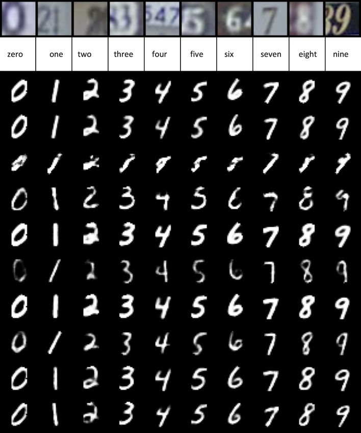
The sum of KL-divergences can be calculated in closed form if prior distribution pθ (z) and unimodal
posterior approximations qφj (z|xj ) are both Gaussian distributed. In this case, this lower bound to
the ELBO L(θ, φ; X) allows the optimization of the ELBO objective in a computationally efficient
way.

3.2   Dynamic Prior

In the regularization term in equation (6), although efficiently optimizable, the unimodal approxima-
tions qφj (z|xj ) are only individually compared to the prior, and no joint objective is involved. We
propose to incoporate the unimodal posterior approximations into the prior through a function f .
Definition 2 (Multimodal Dynamic Prior). The dynamic prior is defined as a function f of the
unimodal approximation functions {qφν (z|xν )}M   ν=1 and a pre-defined distribution pθ (z):

                              pf (z|X) = f ({qφν (z|xν )}M
                                                         ν=1 , pθ (z))                            (7)

The dynamic prior is not a prior distribution in the conventional sense as it does not reflect prior
knowledge of the data, but it incorporates the prior knowledge that all modalities share common
factors. We therefore call it prior due to its role in the ELBO formulation and optimization. As
a function of all the unimodal posterior approximations, the dynamic prior extracts the shared
information and relates the unimodal approximations to it. With this formulation, the objective
is optimized at the same time for a similarity between the function f and the unimodal posterior
approximations. For random sampling, the pre-defined prior pθ (z) is used.

3.3   Jensen-Shannon Divergence

Utilizing the dynamic prior pf (z|X), the sum of KL-divergences in equation (6) can be written as
JS-divergence (see equation (5)) if the function f defines a mixture distribution. To remain a valid
ELBO, the function pf (z|X) needs to be a well-defined prior.
Lemma 1. If the function f of the dynamic prior pf (z|X) defines a mixture distribution of the
unimodal approximation distributions {qφν (z|xν )}M ν=1 , the resulting dynamic prior pM oE (z|X) is
well-defined.

Proof. The proof can be found in appendix B.2.

With Lemma 1, the new multimodal objective L(θ,e φ; X) utilizing the Jensen-Shannon divergence
(Definition 1) can now be directly derived from the ELBO in equation (2).
Lemma 2. The multimodal objective L(θ, e φ; X) utilizing the Jensen-Shannon divergence defined in
equation (4) is a lower bound to the ELBO in equation (2).
                                     L(θ, φ; X) ≥ L(θ,
                                                    e φ; X)                                   (8)

Proof. The lower bound to the ELBO in equation (6) can be rewritten using the dynamic prior
pM oE (z|X):
                                                     M
                                                     X
           L(θ, φ; X) ≥Eqφ (z|X) [log pθ (X|z)] −          πj KL(qφj (z|xj )||pM oE (z|X))
                                                     j=1

                         − πM +1 KL(pθ (z)||pM oE (z|X))
                       =Eqφ (z|X) [log pθ (X|z)] − JSπM +1 ({qφj (z|xj )}M
                                                                         j=1 , pθ (z))

                       =L(θ,
                        e φ; X)                                                                   (9)
Proving that L(θ,
             e φ; X) is a lower bound to the original ELBO formulation in (2) also proves that it
is a lower bound the marginal log-likelihood log pθ (X (i) ). This makes the proposed objective an
ELBO itself.

The objective in equation (4) using the JS-divergence is an intuitive extension of the ELBO formu-
lation to the multimodal case as it relates the unimodal to the multimodal approximation functions
while providing a more expressive prior [27].

                                                 4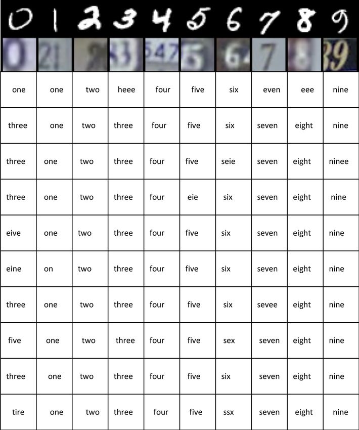
3.4   Generalized Jensen-Shannon Divergence

[20] defines the JS-divergence for the general case of abstract means. This allows to calculate
the JS-divergence not only using an arithmetic mean as in the standard formulation, but any mean
function. Abstract means are a suitable class of functions for aggregating information from different
distributions while being able to handle missing data [20].
Definition 3. The dynamic prior pP oE (z|X) is defined as the geometric mean of the unimodal
posterior approximations {qφν (z|xν )}M ν=1 and the pre-defined distribution pθ (z).

For Gaussian distributed arguments, the geometric mean is again Gaussian distributed and equivalent
to a weighted PoE [8]. The proof that pP oE (z|X) is a well-defined prior can be found in appendix B.3.
Utilizing Definition 3, the JS-divergence in equation (4) can be calculated in closed form. This allows
the optimization of the proposed, multimodal objective L(θ,
                                                         e φ; X) in a computationally efficient way
while also tackling the limitations of previous work outlined in section 2.1. For all experiments, we
use a dynamic prior of the form pP oE (z|X), as given in definition 3.

3.5   Modality-specific Latent Subspaces

We define our latent representations as a combination of modality-specific spaces and a shared,
modality-independent space: z = (S, c) = ({sj }M       j=1 , c). Every xj is modelled to have its own
independent, modality-specific part sj . Additionally, we assume a joint content c for all xj ∈ X
which captures the information that is shared across modalities. S and c are considered conditionally
independent given X. Different to previous work [3, 28], we empirically show that meaningful
representations can be learned in a self-supervised setting by the supervision which is given naturally
for multimodal problems. Building on what we derived in sections 2 and 3, and the assumptions
outlined above, we model the modality-dependent divergence term similarly to the unimodal setting as
there is no intermodality relationship associated with them. Applying these assumptions to Equation
(4), it follows (for details, please see appendix B.4):
                      M
                      X
       L(θ,
       e φ; X) =            Eqφc (c|X) [Eqφs       (sj |xj ) [log pθ (xj |sj , c)]]                      (10)
                                               j
                      j=1
                           M
                           X
                       −         DKL (qφsj (sj |xj )||pθ (sj )) − JSπM +1 ({qφcj (c|xj )}M
                                                                                         j=1 , pθ (c))
                           j=1

The objective in Equation (4) is split further into two different divergence terms: The JS-divergence is
used only for the multimodal latent factors c, while modality-independent terms sj are part of a sum
of KL-divergences. Following the common line in VAE-research, the variational approximation func-
tions qφcj (cj |xj ) and qφsj (sj |xj ), as well as the generative models pθ (xj |sj , c) are parameterized
by neural networks.

4     Experiments & Results
We carry out experiments on two different datasets. For the experiment we use a matching digits
dataset consisting of MNIST [15] and SVHN [18] images with an additional text modality. This
experiment provides empirical evidence on a method’s generalizability to more than two modalities.
The second experiment is carried out on the challenging CelebA faces dataset [17] with additional
text describing the attributes of the shown face. The CelebA dataset is highly imbalanced regarding
the distribution of attributes which poses additional challenges for generative models.

4.1   Evaluation

We evaluate the quality models with respect to the multimodal wish-list introduced in section 1. To
assess the discriminative capabilities of a model, we evaluate the latent representations with respect to
the input data’s semantic information. We employ a linear classifier on the unimodal and multimodal
posterior approximations. To assess the generative performance, we evaluate generated samples
according to their quality and coherence. Generation should be coherent across all modalities with
respect to shared information. Conditionally generated samples should be coherent with the input

                                                            5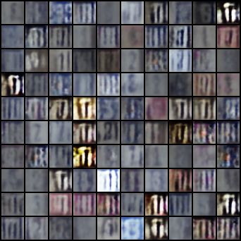
(a) mmJSD (MS): M,S → T                       (b) mmJSD (MS): M,T → S               (c) mmJSD (MS): S,T → M
Figure 1: Qualitative results for missing data estimation. Each row is generated by a single, random
style and the information inferred from the available modalities in the first two rows. This allows
for the generation of samples with coherent, random styles across multiple contents (see Table 1 for
explanation of abbreviations).
Table 1: Classification accuracy of the learned latent representations using a linear classifier. We
evaluate all subsets of modalities for which we use the following abbreviations: M: MNIST; S:
SVHN; T: Text; M,S: MNIST and SVHN; M,T: MNIST and Text; S,T: SVHN and Text; Joint: all
modalities. (MS) names the models with modality-specific latent subspaces.

                       M ODEL               M        S       T      M,S     M,T      S,T     J OINT
                       MVAE                0.85    0.20    0.58     0.80    0.92    0.46      0.90
                       MMVAE               0.96    0.81    0.99     0.89    0.97    0.90      0.93
                       MM JSD              0.97    0.82    0.99     0.93    0.99    0.92      0.98
                       MVAE (MS)           0.86    0.28    0.78     0.82    0.94    0.64      0.92
                       MMVAE (MS)          0.96    0.81    0.99     0.89    0.98    0.91      0.92
                       MM JSD (MS)         0.98    0.85    0.99     0.94    0.98    0.94      0.99

data, randomly generated samples with each other. For every data type, we use a classifier which was
trained on the original training set [22] to evaluate the coherence of generated samples. To assess
the quality of generated samples, we use the precision and recall metric for generative models [23]
where precision defines the quality and recall the diversity of the generated samples. In addition, we
evaluate all models regarding their test set log-likelihoods.
We compare the proposed method to two state-of-the-art models: the MVAE model [30] and the
MMVAE model [24] described in section 2.1. We use the same encoder and decoder networks and
the same number of parameters for all methods. Implementation details for all experiments together
with a comparison of runtimes can be found in appendix C.2.

4.2        MNIST-SVHN-Text

Previous works on scalable, multimodal methods performed no evaluation on more than two modali-
ties1 . We use the MNIST-SVHN dataset [24] as basis. To this dataset, we add an additional, text-based
modality. The texts consist of strings which name the digit in English where the start index of the
word is chosen at random to have more diversity in the data. To evaluate the effect of the dynamic
prior as well as modality-specific latent subspaces, we first compare models with a single shared
latent space. In a second comparison, we add modality-specific subspaces to all models (for these
experiments, we add a (MS)-suffix to the model names). This allows us to assess and evaluate the
contribution of the dynamic prior as well as modality-specific subspaces. Different subspace sizes are
compared in C.2.
      1
          [30] designed a multimodal experiment for the CelebA dataset where every attribute is considered a modality.

                                                            6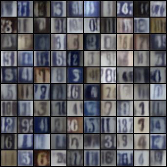
Table 2: Classification accuracy of generated samples on MNIST-SVHN-Text. In case of conditional
generation, the letter above the horizontal line indicates the modality which is generated based on the
different sets of modalities below the horizontal line.

                                                M                                   S                         T
   M ODEL            R ANDOM         S           T          S,T         M           T     M,T          M      S       M,S
   MVAE                0.72        0.17       0.14         0.22       0.37       0.30     0.86        0.20   0.12     0.22
   MMVAE               0.54        0.82       0.99         0.91       0.32       0.30     0.31        0.96   0.83     0.90
   MM JSD              0.60        0.82       0.99         0.95       0.37       0.36     0.48        0.97   0.83     0.92
   MVAE (MS)           0.74        0.16       0.17         0.25       0.35       0.37     0.85        0.24   0.14     0.26
   MMVAE (MS)          0.67        0.77       0.97         0.86       0.88       0.93     0.90        0.82   0.70     0.76
   MM JSD (MS)         0.66        0.80       0.97         0.93       0.89       0.93     0.92        0.92   0.79     0.86

Table 3: Quality of generated samples on MNIST-SVHN-Text. We report the average precision based
on the precision-recall metric for generative models (higher is better) for conditionally and randomly
generated image data (R: Random Generation).

                                                M                                               S
            M ODEL             S          T          S,T          R          M           T           M, T     R
            MVAE              0.62       0.62        0.58        0.62       0.33         0.34         0.22   0.33
            MMVAE             0.22       0.09        0.18        0.35       0.005       0.006        0.006   0.27
            MM JSD            0.19       0.09        0.16        0.15       0.05         0.01         0.06   0.09
            MVAE (MS)         0.60       0.59        0.50        0.60       0.30        0.33         0.17    0.29
            MMVAE (MS)        0.62       0.63        0.63        0.52       0.21        0.20         0.20    0.19
            MM JSD (MS)       0.62       0.64        0.64        0.30       0.21        0.22         0.22    0.17

Table 1 and Table 2 demonstrate that the proposed mmJSD objective generalizes better to three
modalities than previous work. The difficulty of the MVAE objective in optimizing the unimodal
posterior approximation is reflected in the coherence numbers of missing data types and the latent
representation classification. Although MMVAE is able to produce good results if only a single data
type is given, the model cannot leverage the additional information of multiple available observations.
Given multiple modalities, the corresponding performance numbers are the arithmetic mean of their
unimodal pendants. The mmJSD model is able to achieve state-of-the-art performance in optimizing
the unimodal posteriors as well as outperforming previous work in leveraging multiple modalities
thanks to the dynamic prior. The introduction of modality-specific subspaces increases the coherence
of the difficult SVHN modality for MMVAE and mmJSD. More importantly, modality-specific latent
spaces improve the quality of the generated samples for all modalities (see Table 3). Figure 1 shows
qualitative results. Table 4 provides evidence that the high coherence of generated samples of the
mmJSD model are not traded off against test set log-likelihoods. It also shows that MVAE is able to
learn the statistics of a dataset well, but not to preserve the content in case of missing modalities.

Table 4: Test set log-likelihoods on MNIST-SVHN-Text. We report the log-likelihood of the joint
generative model pθ (X) and the log-likelihoods of the joint generative model conditioned on the
variational posterior of subsets of modalities qφK (z|XK ). (xM : MNIST; xS : SVHN; xT : Text;
X = (xM , xS , xT )).

    M ODEL              X      X|xM           X|xS           X|xT           X|xM , xS        X|xM , xT        X|xS , xT
    MVAE              -1864     -2002           -1936        -2040            -1881                 -1970         -1908
    MMVAE             -1916     -2213           -1911        -2250            -2062                 -2231         -2080
    MM JSD            -1961     -2175           -1955        -2249            -2000                 -2121         -2004
    MVAE (MS)         -1870     -1999           -1937        -2033            -1886                 -1971         -1909
    MMVAE (MS)        -1893     -1982           -1934        -1995            -1905                 -1958         -1915
    MM JSD (MS)       -1900     -1994           -1944        -2006            -1907                 -1968         -1918

                                                             7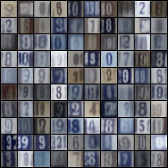
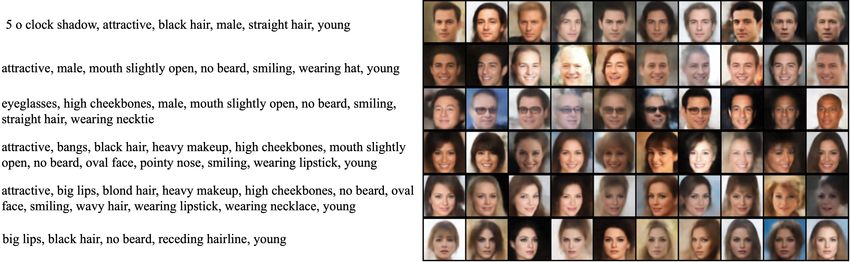
Figure 2: Qualitative Results of CelebA faces which were conditionally generated based on text
strings using mmJSD.

4.3   Bimodal CelebA

Every CelebA image is labelled according to 40 attributes. We extend the dataset with an additional
text modality describing the face in the image using the labelled attributes. Examples of created
strings can be seen in Figure 2. Any negative attribute is completely absent in the string. This is
different and more difficult to learn than negated attributes as there is no fixed position for a certain
attribute in a string which introduces additional variability in the data. Figure 2 shows qualitative
results for images which are generated conditioned on text samples. Every row of images is based
on the text next to it. As the labelled attributes are not capturing all possible variation of a face, we
generate 10 images with randomly sampled image-specific information to capture the distribution of
information which is not encoded in the shared latent space. The imbalance of some attributes effects
the generative process. Rare and subtle attributes like eyeglasses are difficult to learn while frequent
attributes like gender and smiling are well learnt.
Table 5 demonstrates the superior performance of the proposed mmJSD objective compared to
previous work on the challening bimodal CelebA dataset. The classification results regarding the
individual attributes can be found in appendix C.3.

Table 5: Classfication results on the bimodal CelebA experiment. For latent representations and
conditionally generated samples, we report the mean average precision over all attributes (I: Image;
T: Text; Joint: I and T).

                                      L ATENT R EPRESENTATION        G ENERATION
                    M ODEL              I       T        J OINT     I→T       T→I
                    MVAE (MS)         0.42    0.45       0.44        0.32     0.30
                    MMVAE (MS)        0.43    0.45       0.42        0.30     0.36
                    MM JSD (MS)       0.48    0.59       0.57        0.32     0.42

5     Conclusion

In this work, we propose a novel generative model for learning from multimodal data. Our con-
tributions are fourfold: (i) we formulate a new multimodal objective using a dynamic prior. (ii)
We propose to use the JS-divergence for multiple distributions as a divergence measure for multi-
modal data. This measure enables direct optimization of the unimodal as well as the joint latent
approximation functions. (iii) We prove that the proposed mmJSD objective constitutes an ELBO for
multiple data types. (iv) With the introduction of modality-specific latent spaces, we show empirically
the improvement in quality of generated samples. Additionally, we demonstrate that the proposed
method does not need any additional training objectives while reaching state-of-the-art or superior
performance compared to recently proposed, scalable, multimodal generative models. In future work,
we would like to further investigate which functions f would serve well as prior function and we will
apply our proposed model in the medical domain.

                                                     8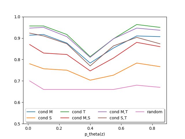
6   Broader Impact
Learning from multiple data types offers many potential applications and opportunities as multiple
data types naturally co-occur. We intend to apply our model in the medical domain in future work,
and we will focus here on the impact our model might have in the medical application area. Models
that are capable of dealing with large-scale multi-modal data are extremely important in the field of
computational medicine and clinical data analysis. The recent developments in medical information
technology have resulted in an overwhelming amount of multi-modal data available for every single
patient. A patient visit at a hospital may result in tens of thousands of measurements and structured
information, including clinical factors, diagnostic imaging, lab tests, genomic and proteomic tests,
and hospitals may see thousands of patients each year. The ultimate aim is to use all this vast
information for a medical treatment tailored to the needs of an individual patient. To turn the vision of
precision medicine into reality, there is an urgent need for the integration of the multi-modal patient
data currently available for improved disease diagnosis, prognosis and therapy outcome prediction.
Instead of learning on one data set exclusively, as for example just on images or just on genetics,
the aim is to improve learning and enhance personalized treatment by using as much information as
possible for every patient. First steps in this direction have been successful, but so far a major hurdle
has been the huge amount of heterogeneous data with many missing data points which is collected
for every patient.
With this work, we lay the theoretical foundation for the analysis of large-scale multi-modal data.
We focus on a self-supervised approach as collecting labels for large datasets of multiple data types
is expensive and becomes quickly infeasible with a growing number of modalities. Self-supervised
approaches have the potential to overcome the need for excessive labelling and the bias coming from
these labels. In this work, we extensively tested the model in controlled environments. In future work,
we will apply our proposed model to medical multi-modal data with the goal of gaining insights and
making predictions about disease phenotypes, disease progression and response to treatment.

References
 [1] J. A. Aslam and V. Pavlu. Query hardness estimation using Jensen-Shannon divergence among
     multiple scoring functions. In European conference on information retrieval, pages 198–209.
     Springer, 2007.
 [2] T. Baltrušaitis, C. Ahuja, and L.-P. Morency. Multimodal machine learning: A survey and
     taxonomy. IEEE Transactions on Pattern Analysis and Machine Intelligence, 41(2):423–443,
     2018.
 [3] D. Bouchacourt, R. Tomioka, and S. Nowozin. Multi-level variational autoencoder: Learning
     disentangled representations from grouped observations. In Thirty-Second AAAI Conference on
     Artificial Intelligence, 2018.
 [4] Y. Burda, R. Grosse, and R. Salakhutdinov. Importance Weighted Autoencoders. pages 1–14,
     2015. URL http://arxiv.org/abs/1509.00519.
 [5] H. Fang, S. Gupta, F. Iandola, R. K. Srivastava, L. Deng, P. Dollár, J. Gao, X. He, M. Mitchell,
     J. C. Platt, and others. From captions to visual concepts and back. In Proceedings of the IEEE
     conference on computer vision and pattern recognition, pages 1473–1482, 2015.
 [6] K. He, X. Zhang, S. Ren, and J. Sun. Deep residual learning for image recognition. In
     Proceedings of the IEEE conference on computer vision and pattern recognition, pages 770–
     778, 2016.
 [7] J. R. Hershey and P. A. Olsen. Approximating the Kullback Leibler divergence between
     Gaussian mixture models. In 2007 IEEE International Conference on Acoustics, Speech and
     Signal Processing-ICASSP’07, volume 4, pages IV–317. IEEE, 2007.
 [8] G. E. Hinton. Products of experts. 1999.
 [9] W.-N. Hsu and J. Glass. Disentangling by Partitioning: A Representation Learning Framework
     for Multimodal Sensory Data. 2018. URL http://arxiv.org/abs/1805.11264.
[10] X. Huang, M.-Y. Liu, S. Belongie, and J. Kautz. Multimodal unsupervised image-to-image
     translation. In Proceedings of the European Conference on Computer Vision (ECCV), pages
     172–189, 2018.

                                                   9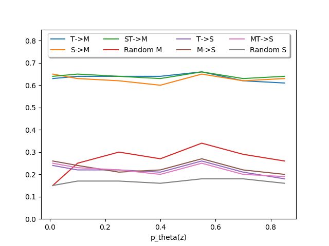
[11] A. Karpathy and L. Fei-Fei. Deep visual-semantic alignments for generating image descriptions.
     In Proceedings of the IEEE conference on computer vision and pattern recognition, pages
     3128–3137, 2015.
[12] D. P. Kingma and J. Ba. Adam: A method for stochastic optimization. arXiv preprint
     arXiv:1412.6980, 2014.
[13] D. P. Kingma and M. Welling. Auto-Encoding Variational Bayes. (Ml):1–14, 2013. URL
     http://arxiv.org/abs/1312.6114.
[14] R. Kurle, S. Günnemann, and P. van der Smagt. Multi-Source Neural Variational Inference.
     2018. URL http://arxiv.org/abs/1811.04451.
[15] Y. LeCun and C. Cortes. {MNIST} handwritten digit database. 2010. URL http://yann.
     lecun.com/exdb/mnist/.
[16] J. Lin. Divergence measures based on the Shannon entropy. IEEE Transactions on Information
     theory, 37(1):145–151, 1991.
[17] Z. Liu, P. Luo, X. Wang, and X. Tang. Deep Learning Face Attributes in the Wild. In The IEEE
     International Conference on Computer Vision (ICCV), 2015.
[18] Y. Netzer, T. Wang, A. Coates, A. Bissacco, B. Wu, and A. Y. Ng. Reading digits in natural
     images with unsupervised feature learning. 2011.
[19] J. Ngiam, A. Khosla, M. Kim, J. Nam, H. Lee, and A. Y. Ng. Multimodal deep learning.
     In Proceedings of the 28th international conference on machine learning (ICML-11), pages
     689–696, 2011.
[20] F. Nielsen. On the Jensen-Shannon symmetrization of distances relying on abstract means.
     Entropy, 2019. ISSN 10994300. doi: 10.3390/e21050485.
[21] F. Pedregosa, G. Varoquaux, A. Gramfort, V. Michel, B. Thirion, O. Grisel, M. Blondel,
     P. Prettenhofer, R. Weiss, V. Dubourg, and others. Scikit-learn: Machine learning in Python.
     Journal of machine learning research, 12(Oct):2825–2830, 2011.
[22] S. Ravuri and O. Vinyals. Classification accuracy score for conditional generative models. In
     Advances in Neural Information Processing Systems, pages 12247–12258, 2019.
[23] M. S. M. Sajjadi, O. Bachem, M. Lucic, O. Bousquet, and S. Gelly. Assessing generative
     models via precision and recall. In Advances in Neural Information Processing Systems, pages
     5228–5237, 2018.
[24] Y. Shi, N. Siddharth, B. Paige, and P. Torr. Variational Mixture-of-Experts Autoencoders for
     Multi-Modal Deep Generative Models. In Advances in Neural Information Processing Systems,
     pages 15692–15703, 2019.
[25] M. Suzuki, K. Nakayama, and Y. Matsuo. Joint Multimodal Learning with Deep Generative
     Models. pages 1–12, 2016. URL http://arxiv.org/abs/1611.01891.
[26] Y. Tian and J. Engel. Latent translation: Crossing modalities by bridging generative models.
     arXiv preprint arXiv:1902.08261, 2019.
[27] J. M. Tomczak and M. Welling. VAE with a VampPrior. arXiv preprint arXiv:1705.07120,
     2017.
[28] Y.-H. H. Tsai, P. P. Liang, A. Zadeh, L.-P. Morency, and R. Salakhutdinov. Learning factorized
     multimodal representations. arXiv preprint arXiv:1806.06176, 2018.
[29] R. Vedantam, I. Fischer, J. Huang, and K. Murphy. Generative models of visually grounded
     imagination. arXiv preprint arXiv:1705.10762, 2017.
[30] M. Wu and N. Goodman. Multimodal Generative Models for Scalable Weakly-Supervised
     Learning. (Nips), 2018. URL http://arxiv.org/abs/1802.05335.
[31] A. Zadeh, M. Chen, S. Poria, E. Cambria, and L.-P. Morency. Tensor fusion network for
     multimodal sentiment analysis. arXiv preprint arXiv:1707.07250, 2017.
[32] J.-Y. Zhu, T. Park, P. Isola, and A. A. Efros. Unpaired Image-To-Image Translation Using
     Cycle-Consistent Adversarial Networks. In The IEEE International Conference on Computer
     Vision (ICCV), 2017.

                                               10
In the supplementary material section, we provide additional mathematical derivations, implementa-
tion details and results which could not be put in the main paper due to space restrictions.
A Theoretical Background
The ELBO L(θ, φ; X) can be derived by reformulating the KL-divergence between the joint posterior
approximation function qφ (z|X) and the true posterior distribution pθ (z|X):
Z
qφ (z|X)
KL(qφ (z|X)||pθ (z|X)) = qφ (z|X) log dz
z pθ (z|X)
Z
qφ (z|X)pθ (X)
= qφ (z|X) log dz
z pθ (X, z)
=Eqφ [log(qφ (z|X)) − log(pθ (X, z))] + log(pθ (X)) (11)
It follows:
log pθ (X) = KL(qφ (z|X)||pθ (z|X)) − Eqφ [log(qφ (z|X)) − log(pθ (X, z))] + log(pθ (X))
(12)
From the non-negativity of the KL-divergence, it directly follows:
L(θ, φ; X) =Eqφ (z|X) [log(pθ (X|z)] − KL(qφ (z|X)||pθ (z)) (13)
In the absence of one or multiple data types, we would still like to be able to approximate the true
multimodal posterior distribution pθ (z|X). However, we are only able to approximate the posterior
by a variational function qφ (z|XK ) with K ≤ M . In addition, for different samples, different
modalities might be missing. The derivation of the ELBO formulation changes accordingly:
Z
qφ (z|XK )
KL(qφK (z|XK )||pθ (z|X)) = qφ (z|XK ) log dz
z pθ (z|X)
Z
qφ (z|XK )pθ (X)
= qφ (z|XK ) log dz
z pθ (X, z)
=Eqφ [log(qφ (z|XK )) − log(pθ (X, z))] + log(pθ (X)) (14)
From where it again follows:
LK (θ, φK , X) =Eqφ (z|XK ) [log(pθ (X|z)] − KL(qφ (z|XK )||pθ (z)) (15)
B Multimodal Jensen-Shannon Divergence Objective
In this section, we provide the proofs to the Lemmas which were introduced in the main paper. Due
to space restrictions, the proofs of these Lemmas had to be moved to the appendix.
B.1 Upper bound to the KL-divergence of a mixture distribution
Lemma 3 (Joint Approximation Function). Under the assumption of qφ (z|{xj }M j=1 ) being a mixture
model of the unimodal variational posterior approximations qφj (z|xj ), the KL-divergence of the
multimodal variational posterior approximation qφ (z|{xj }M
j=1 ) is a lower bound for the weighted
sum of the KL-divergences of the unimodal variational approximation functions qφj (z|xj ):
M
X M
X
KL( πj qφj (z|xj )||pθ (z)) ≤ πj KL(qφj (z|xj )||pθ (z)) (16)
j=1 j=1
Proof. Lemma 3 follows directly from the strict convexity of g(t) = t log t.
11B.2 MoE-Prior
Definition 4 (MoE-Prior). The prior pM oE (z|X) is defined as follows:
M
X
pM oE (z|X) = πν qφν (z|xν ) + πM +1 pθ (z) (17)
ν=1
where qφν (z|xν ) are again the unimodal approximation functionsP and pθ (z) is a pre-defined, param-
eterizable distribution. The mixture weights π sum to one, i.e. πj = 1.
We prove that the MoE-prior pM oE (z|X) is a well-defined prior (see Lemma 1):
Proof. To be a well-defined prior, pM oE (z|X) must satisfy the following condition:
Z
pM oE (z|X)dz = 1 (18)
Therefore,
Z M
!
X
πν qφν (z|xν ) + πM +1 pθ (z) dz
ν=1
M
X Z Z
= πν qφν (z|xν )dz + πM +1 pθ (z)dz
ν=1
M
X
= πν + πM +1 = 1 (19)
ν=1
The unimodal approximation functions qφν (z|xν ) as R well as the pre-defined distribution pθ (z)
R well-defined probability distributions. Hence, qφν (z|xν )dz = 1 for all qφν (z|xν ) and
are
pθ (z)dz = 1. The last line in equation 19 follows from the assumptions. Therefore, equation (17)
is a well-defined prior.
B.3 PoE-Prior
Lemma 4. Under the assumption that all qφν (z|xν ) are Gaussian distributed by
N (µν (xν ), σν2 (xν )I), pP oE (z|X) is Gaussian distributed:
2
pP oE (z|X) ∼ N (µGM , σGM I) (20)
2
where µGM and σGM I are defined as follows:
M
X +1 M
X +1
2
σGM I =( πk σk2 I)−1 , µGM = 2
(σGM I) πk (σk2 I)−1 µk (21)
k=1 k=1
which makes pP oE (z|X) a well-defined prior.
Proof. As pP oE (z|X) is Gaussian distributed, it follows immediately that pP oE (z|X) is a well-
defined dynamic prior.
B.4 Factorization of Representations
We mostly base our derivation of factorized representations on the paper by Bouchacourt et al. [3].
Tsai et al. [28] and Hsu and Glass [9] used a similar idea. A set X of modalities can be seen as
group and analogous every modality as a member of a group. We model every xj to have its own
modality-specific latent code sj ∈ S.
S = (sj , ∀xj ∈ X) (22)
From Equation (22), we see that S is the collection of all modality-specific latent variables for the set
X. Contrary to this, the modality-invariant latent code c is shared between all modalities xj of the
12set X. Also like Bouchacourt et al. [3], we model the variational approximation function qφ (S, c) to
be conditionally independent given X, i.e.:
qφ (S, c) = qφS (S|X)qφc (c|X) (23)
From the assumptions it is clear that qφS factorizes:
M
Y
qφS (S|X) = qφsj (sj |xj ) (24)
j=1
From Equation (24) and the fact that the multimodal relationships are only modelled by the latent
factor c, it is reasonable to only apply the mmJSD objective to c. It follows:
L(θ, φ; X) =Eqφ (z|X) [log pθ (X|z)] − KL(qφ (z|X)||pθ (z))
=Eqφ (S,c|X) [log pθ (X|S, c)] − KL(qφ (S, c|X)||pθ (S, c))
=Eqφ (S,c|X) [log pθ (X|S, c)] − KL(qφS (S|X)||pθ (S)) − KL(qφc (c|X)||pf (c))
M
X
=Eqφ (S,c|X) [log pθ (X|S, c)] − KL(qφsj (sj |xj )||pθ (sj )) − KL(qφc (c|X)||pf (c))
j=1
(25)
In Equation (25), we can rewrite the KL-divergence which includes c using the multimodal dynamic
prior and the JS-divergence for multiple distributions:
M
X
L(θ,
e φ; X) =Eq (S,c|X) [log pθ (X|S, c)] −
φ
KL(qφsj (sj |xj )||pθ (sj ))
j=1
− JSπM +1 ({qφcj (c|xj )}M
j=1 , pθ (c)) (26)
The expectation over qφ (S, c|X) can be rewritten as a concatenation of expectations over qφc (c|X)
and qφsj (sj |xj ):
Z Z
Eqφ (S,c|X) [log pθ (X|S, c)] = qφ (S, c|X) log pθ (X|S, c)dSdc
Zc S Z
= qφc (c|X) qφS (S|X) log pθ (X|S, c)dSdc
c S
Z M Z
X
= qφc (c|X) qφsj (sj |xj ) log pθ (xj |sj , c)dsj dc
c j=1 sj
M Z
X Z
= qφc (c|X) qφsj (sj |xj ) log pθ (xj |sj , c)dsj dc
j=1 c sj
M
X
= Eqφc (c|X) [Eqφs (sj |xj ) [log pθ (xj |sj , c)]] (27)
j
j=1
From Equation (27), the final form of L(θ,
e φ; X) follows directly:
M
X
L(θ,
e φ; X) = Eqφc (c|X) [Eqφs (sj |xj ) [log pθ (xj |sj , c)]]
j
j=1
M
X
− JSπM +1 ({qφcj (c|xj )}M
j=1 , pθ (c)) − KL(qφsj (sj |xj )||pθ (sj )) (28)
j=1
B.5 JS-divergence as intermodality divergence
Utilizing the JS-divergence as regularization term as proposed in this work has multiple effects on the
training procedure. The first is the introduction of the dynamic prior as described in the main paper.
13Table 6: Layers for MNIST and SVHN classifiers. For MNIST and SVHN, every convolutional layer
is followed by a ReLU activation function. For SVHN, every convolutional layer is followed by a
dropout layer (dropout probability = 0.5). Then, batchnorm is applied followed by a ReLU activation
function. The output activation is a sigmoid function for both classifiers. Specifications (Spec.) name
kernel size, stride, padding and dilation.
MNIST SVHN
Layer Type #F. In #F. Out Spec. Layer Type #F. In #F. Out Spec.
1 conv2d 1 32 (4, 2, 1, 1) 1 conv2d 1 32 (4, 2, 1, 1)
2 conv2d 32 64 (4, 2, 1, 1) 2 conv2d 32 64 (4, 2, 1, 1)
3 conv2d 64 128 (4, 2, 1, 1) 3 conv2d 64 64 (4, 2, 1, 1)
4 linear 128 10 4 conv2d 64 128 (4, 2, 0, 1)
5 linear 128 10
A second effect is the minimization of the intermodality-divergence. The intermodality-divergence is
the difference of the posterior approximations between modalities. For a coherent generation, the
posterior approximations of all modalities should be similar such that - if only a single modality
is given - the decoders of the missing data types are able to generate coherent samples. Using the
JS-divergence as regularization term keeps the unimodal posterior approximations similar to its
mixture distribution. This can be compared to minimizing the divergence between the unimodal
distributions and its mixture which again can be seen as an efficient approximation of minimizing the
M 2 pairwise unimodal divergences, the intermodality-divergences. Wu and Goodman [30] report
problems in optimizing the unimodal posterior approximations. These problems lead to diverging
posterior approximations which again results in bad coherence for missing data generation. Diverging
posterior approximations cannot be handled by the decoders of the missing modality.
C Experiments
In this section we describe the architecture and implementation details of the different experiments.
Additionally, we show more results and ablation studies.
C.1 Evaluation
First we describe the architectures and models used for evaluating classification accuracies.
C.1.1 Latent Representations
To evaluate the learned latent representations, we use a simple logistic regression classifier without
any regularization. We use a predefined model by scikit-learn [21]. Every linear classifier is trained
on a single batch of latent representations. For simplicity, we always take the last batch of the training
set to train the classifier. The trained linear classifier is then used to evaluate the latent representations
of all samples in the test set.
C.1.2 Generated Samples
To evaluate generated samples regarding their content coherence, we classify them according to
the attributes of the dataset. In case of missing data, the estimated data types must coincide with
the available ones according to the attributes present in the available data types. In case of random
generation, generated samples of all modalities must be coincide with each other. To evaluate the
coherence of generated samples, classifiers are trained for every modality. If the detected attributes
for all involved modalities are the same, the generated samples are called coherent. For all modalities,
classifiers are trained on the original, unimodal training set. The architectures of all used classifiers
can be seen in Tables 6 to 8.
14Table 7: Layers for the Text classifier for MNIST-SVHN-Text. The text classifier consists of residual
layers as described by He et al. [6] for 1d-convolutions. The output activation is a sigmoid function.
Specifications (Spec.) name kernel size, stride, padding and dilation.
Layer Type #F. In #F. Out Spec.
1 conv1d 71 128 (1, 1, 1, 1)
2 residual1d 128 192 (4, 2, 1, 1)
3 residual1d 192 256 (4, 2, 1, 1)
4 residual1d 256 256 (4, 2, 1, 1)
5 residual1d 256 128 (4, 2, 0, 1)
6 linear 128 10
Table 8: CelebA Classifiers. The image classifier consists of residual layers as described by He et al.
[6] followed by a linear layer which maps to 40 output neurons representing the 40 attributes. The
text classifier also uses residual layers, but for 1d-convolutions. The output activation is a sigmoid
function for both classifiers. Specifications (Spec.) name kernel size, stride, padding and dilation.
Image Text
Layer Type #F. In #F. Out Spec. Layer Type #F. In #F. Out Spec.
1 conv2d 3 128 (3, 2, 1, 1) 1 conv1d 71 128 (3, 2, 1, 1)
2 res2d 128 256 (4, 2, 1, 1) 2 res1d 128 256 (4, 2, 1, 1)
3 res2d 256 384 (4, 2, 1, 1) 3 res1d 256 384 (4, 2, 1, 1)
4 res2d 384 512 (4, 2, 1, 1) 4 res1d 384 512 (4, 2, 1, 1)
5 res2d 512 640 (4, 2, 0, 1) 5 res1d 512 640 (4, 2, 1, 1)
6 linear 640 40 6 residual1d 640 768 (4, 2, 1, 1)
7 residual1d 768 896 (4, 2, 0, 1)
8 linear 896 40
C.2 MNIST-SVHN-Text
C.2.1 Text Modality
To have an additional modality, we generate text from labels. As a single word is quite easy to learn,
we create strings of length 8 where everything is a blank space except the digit-word. The starting
position of the word is chosen randomly to increase the difficulty of the learning task. Some example
strings can be seen in Table 9.
C.2.2 Implementation Details
For MNIST and SVHN, we use the network architectures also utilized by [24] (see Table 10 and
Table 11). The network architecture used for the Text modality is described in Table 12. For all
encoders, the last layers named a and b are needed to map to µ and σ 2 I of the posterior distribution.
Table 9: Example strings to create an additional text modality for the MNIST-SVHN-Text dataset.
This results in triples of texts and two different image modalities.
six
eight
three
five
nine
zero
four
three
seven
five
15Table 10: MIST: Encoder and Decoder Layers. Every layer is followed by ReLU activation function.
Layers 3a and 3b of the encoder are needed to map to µ and σ 2 I of the approximate posterior
distribution.
Encoder Decoder
Layer Type # Features In # Features Out Layer Type # Features In # Features Out
1 linear 784 400 1 linear 20 400
2a linear 400 20 2 linear 400 784
2b linear 400 20
Table 11: SVHN: Encoder and Decoder Layers. The specifications name kernel size, stride, padding
and dilation. All layers are followed by a ReLU activation function.
Encoder Decoder
Layer Type #F. In #F. Out Spec. Layer Type #F. In #F. Out Spec.
1 conv2d 3 32 (4, 2, 1, 1) 1 linear 20 128
2 conv2d 32 64 (4, 2, 1, 1) 2 convT2d 128 64 (4, 2, 0, 1)
3 conv2d 64 64 (4, 2, 1, 1) 3 convT2d 64 64 (4, 2, 1, 1)
4 conv2d 64 128 (4, 2, 0, 1) 4 convT2d 64 32 (4, 2, 1, 1)
5a linear 128 20 5 convT2d 32 3 (4, 2, 1, 1)
5b linear 128 20
In case of modality-specific sub-spaces, there are four last layers to map to µs and σs2 I and µc and
σc2 I.
To enable a joint latent space, all modalities are mapped to have a 20 dimensional latent space (like in
Shi et al. [24]). For a latent space with modality-specific and -independent sub-spaces, this restriction
is not needed anymore. Only the modality-invariant sub-spaces of all data types must have the same
number of latent dimensions. Nevertheless, we create modality-specific sub-spaces of the same size
for all modalities. For the results reported in the main text, we set it to 4. To have an equal number of
parameters as in the experiment with only a shared latent space, we set the shared latent space to 16
dimensions. This allows for a fair comparison between the two variants regarding the capacity of
the latent space. See appendix C.2.5 and Figure 5 for a detailed comparison regarding the size of
the modality specific-subspaces. Modality-specific sub-spaces are a possibility to account for the
difficulty of every data type.
The image modalities are modelled with a Laplace likelihood and the text modality is modelled
with a categorical likelihood. The likelihood-scaling is done according to the data size of every
modality. The weight of the largest data type, i.e. SVHN, is set to 1.0. The weight for MNIST is
given by size(SV HN )/size(M N IST ) and the text weight by size(SV HN )/size(T ext). This
scaling scheme stays the same for all experiments. The weight of the unimodal posteriors are equally
weighted to form the joint distribution. This is true for MMVAE and mmJSD. For MVAE, the
posteriors are weighted according to the inverse of their variance. For mmJSD, all modalities and
Table 12: Text for MNIST-SVHN-Text: Encoder and Decoder Layers. The specifications name kernel
size, stride, padding and dilation. All layers are followed by a ReLU activation function.
Encoder Decoder
Layer Type #F. In #F. Out Spec. Layer Type #F. In #F. Out Spec.
1 conv1d 71 128 (1, 1, 0, 1) 1 linear 20 128
2 conv1d 128 128 (4, 2, 1, 1) 2 convT1d 128 128 (4, 1, 0, 1)
3 conv1d 128 128 (4, 2, 0, 1) 3 convT1d 128 128 (4, 2, 1, 1)
4a linear 128 20 4 convT1d 128 71 (1, 1, 0, 1)
4b linear 128 20
16(a) Latent Representation Classification (b) Generation Coherence
(c) Quality of Samples
Figure 3: Comparison of different β values with respect to generation coherence, quality of latent
representations (measured in accuracy) and quality of generated samples (measured in precision-recall
for generative models).
the pre-defined distribution are weighted 0.25. We keep this for all experiments reported in the main
paper. See appendix C.2.6 and Figure 6 for a more detailed analysis of distribution weights.
For all experiments, we set β to 5.0. For all experiments with modality-specific subspaces, the β for
the modality-specific subspaces is set equal to the number of modalities, i.e. 3. Additionally, the β
for the text modality is set to 5.0, for the other 2 modalities it is set to 1.0. The evaluation of different
β-values shows the stability of the model according to this hyper-parameter (see Figure 3).
All unimodal posterior approximations are assumed to be Gaussian distributed N (µν (xν ), σν2 (xν )I),
as well as the pre-defined distribution pθ (z) which is defined as N (0, I).
For training, we use a batch size of 256 and a starting learning rate of 0.001 together with an ADAM
optimizer [12]. We pair every MNIST image with 20 SVHN images which increases the dataset size
by a factor of 20. We train our models for 50 epochs in case of a shared latent space only. In case of
modality-specific subspaces we train the models for 100 epochs. This is the same for all methods.
C.2.3 Qualitative Results
Figure 4 shows qualitative results for the random generation of MNIST and SVHN samples.
C.2.4 Comparison to Shi et al.
The results reported in Shi et al. [24]’s paper with the MMVAE model rely heavily on importance
sampling (IS) (as can be seen by comparing to the numbers of a model without IS reported in their
appendix). The IS-based objective [4] is a different objective and difficult to compare to models
without an IS-based objective. Hence, to have a fair comparison between all models we compared all
models without IS-based objective in the main paper. The focus of the paper was on the different joint
17(a) MVAE: MNIST (b) MMVAE: MNIST (c) mmJSD: MNIST
(d) MVAE: SVHN (e) MMVAE: SVHN (f) mmJSD: SVHN
Figure 4: Qualitative results for random generation.
Table 13: Comparison of training times on the MNIST-SVHN-Text dataset. (I=30) names the model
with 30 importance samples.
M ODEL # EPOCHS RUNTIME
MVAE 50 3 H 01 MIN
MMVAE 50 2 H 01 MIN
MMVAE (I=30) 30 15 H 15 MIN
MM JSD 50 2 H 16 MIN
MVAE (MS) 100 6 H 15 MIN
MMVAE (MS) 100 4 H 10 MIN
MM JSD (MS) 100 4 H 36 MIN
posterior approximation functions and the corresponding ELBO which should reflect the problems of
a multimodal model.
For completeness we compare the proposed model to the IS-based MMVAE model here in the
appendix. Table 13 shows the training times for the different models. Although the MMVAE (I=30)
only needs 30 training epochs for convergence, these 30 epochs take approximately 3 times as long
as for the other models without importance sampling. (I=30) names the model with 30 importance
samples. What is also adding up to the training time for the MMVAE (I=30) model is the M 2 paths
through the decoder. The MMVAE model and mmJSD need approximately the same time until
training is finished. MVAE takes longer as the training objective is a combination of ELBOs instead
of a single objective.
Tables 14, 15 and 16 show that the models without any importance samples achieve state-of-the-art
performance compared to the MMVAE model using importance samples. Using modality-specific
subspaces seems to have a similar effect towards test set log-likelihood performance as using
importance samples with a much lower impact on computational efficiency as it can be seen in the
comparison of training times in Table 13.
18Table 14: Classification accuracy of the learned latent representations using a linear classifier. We
evaluate all subsets of modalities for which we use the following abbreviations: M: MNIST; S:
SVHN; T: Text; M,S: MNIST and SVHN; M,T: MNIST and Text; S,T: SVHN and Text; Joint: all
modalities. (MS) names the models with modality-specific latent subspaces. (I=30) names the model
with 30 importance samples.
M ODEL M S T M,S M,T S,T J OINT
MMVAE 0.96 0.81 0.99 0.89 0.97 0.90 0.93
MMVAE (I=30) 0.92 0.67 0.99 0.80 0.96 0.83 0.86
MM JSD 0.97 0.82 0.99 0.93 0.99 0.92 0.98
MMVAE (MS) 0.96 0.81 0.99 0.89 0.98 0.91 0.92
MM JSD
(MS) 0.98 0.85 0.99 0.94 0.98 0.94 0.99
Table 15: Classification accuracy of generated samples on MNIST-SVHN-Text. In case of conditional
generation, the letter above the horizontal line indicates the modality which is generated based on the
different sets of modalities below the horizontal line. (I=30) names the model with 30 importance
samples.
M S T
M ODEL R ANDOM S T S,T M T M,T M S M,S
MMVAE (I=30) 0.60 0.71 0.99 0.85 0.76 0.68 0.72 0.95 0.73 0.84
MMVAE 0.54 0.82 0.99 0.91 0.32 0.30 0.31 0.96 0.83 0.90
MM JSD 0.60 0.82 0.99 0.95 0.37 0.36 0.48 0.97 0.83 0.92
MMVAE (MS) 0.67 0.77 0.97 0.86 0.88 0.93 0.90 0.82 0.70 0.76
MM JSD
(MS) 0.66 0.80 0.97 0.93 0.89 0.93 0.92 0.92 0.79 0.86
C.2.5 Modality-Specific Subspaces
The introduction of modality-specific subspaces introduces an additional degree of freedom. In
Figure 5, we show a comparison of different modality-specific subspace sizes. The size is the
same for all modalities. Also, the total number of latent dimensions is constant, i.e. the number
of dimensions in the modality-specific subspaces is subtracted from the shared latent space. If we
have modality-specific latent spaces of size 2, the shared latent space is of size 18. This allows
to ensure that the capacity of latent spaces stays constant. Figure 5 shows that the introduction of
modality-specific subspaces only has minor effect on the quality of learned representations, despite
the lower number of dimensions in the shared space. Generation coherence suffers with increasing
number of modality-specific dimensions, but the quality of samples improves. We guess that the
coherence becomes lower due to information which is shared between modalities but encoded in
modality-specific spaces. In future work, we are interested in finding better schemes to identify
shared and modality-specific information.
C.2.6 Weight of predefined distribution in JS-divergence
We empirically analyzed the influence of different weights of the pre-defined distribution pθ (z)
in the JS-divergence. Figure 6 shows the results. We see the constant performance regarding the
latent representations and the quality of samples. In future work we would like to study the drop in
performance regarding the coherence of samples if the weight of the pre-defined distribution pθ (z) is
around 0.4.
C.3 CelebA
C.3.1 Bimodal Dataset
Every face in the dataset is labelled with 40 attributes. For the text modality, we create text strings
from these attributes. The text modality is a concatenation of available attributes into a comma-
separated list. Underline characters are replaced by a blank space. We create strings of length 256
19You can also read